Bias determination and precision validation of ozone profiles from MIPAS-Envisat retrieved with the IMK-IAA processor

(1)

HAL Id: hal-00296286

https://hal.archives-ouvertes.fr/hal-00296286

Submitted on 11 Jul 2007

HAL is a multi-disciplinary open access

archive for the deposit and dissemination of

sci-entific research documents, whether they are

pub-lished or not. The documents may come from

teaching and research institutions in France or

abroad, or from public or private research centers.

L’archive ouverte pluridisciplinaire HAL, est

destinée au dépôt et à la diffusion de documents

scientifiques de niveau recherche, publiés ou non,

émanant des établissements d’enseignement et de

recherche français ou étrangers, des laboratoires

publics ou privés.

profiles from MIPAS-Envisat retrieved with the

IMK-IAA processor

T. Steck, T. von Clarmann, H. Fischer, B. Funke, N. Glatthor, U. Grabowski,

M. Höpfner, S. Kellmann, M. Kiefer, A. Linden, et al.

To cite this version:

T. Steck, T. von Clarmann, H. Fischer, B. Funke, N. Glatthor, et al.. Bias determination and precision

validation of ozone profiles from MIPAS-Envisat retrieved with the IMK-IAA processor. Atmospheric

Chemistry and Physics, European Geosciences Union, 2007, 7 (13), pp.3639-3662. �hal-00296286�

(2)

www.atmos-chem-phys.net/7/3639/2007/ © Author(s) 2007. This work is licensed under a Creative Commons License.

Chemistry

and Physics

Bias determination and precision validation of ozone profiles from

MIPAS-Envisat retrieved with the IMK-IAA processor

T. Steck1, T. von Clarmann1, H. Fischer1, B. Funke2, N. Glatthor1, U. Grabowski1, M. H¨opfner1, S. Kellmann1, M. Kiefer1, A. Linden1, M. Milz1, G. P. Stiller1, D. Y. Wang3, M. Allaart4, Th. Blumenstock1, P. von der Gathen5, G. Hansen6, F. Hase1, G. Hochschild1, G. Kopp1, E. Kyr¨o7, H. Oelhaf1, U. Raffalski8, A. Redondas Marrero9, E. Remsberg10, J. Russell III11, K. Stebel6, W. Steinbrecht12, G. Wetzel1, M. Yela13, and G. Zhang1

1_{Institut f¨ur Meteorologie und Klimaforschung, Forschungszentrum Karlsruhe, Germany} 2_{Instituto de Astrof´ısica de Andaluc´ıa, Granada, Spain}

3_{Physics Department, University of New Brunswick, Canada}

4_{KNMI (Royal Netherlands Meteorological Institute), De Bilt, The Netherlands} 5_{Alfred Wegener Institute for Polar and Marine Research, Potsdam, Germany}

6_{Norwegian Institute for Air Research (NILU), Polar Environmental Centre, Tromsø, Norway} 7_{FMI-Arctic Research Centre, Sodankyl¨a, Finland}

8_{Swedish Institute of Space Physics (IRF), Kiruna, Sweden}

9_{Instituto Nacional de Meteorologia (INM), Santa Cruz de Tenerife, Spain}

10_{Atmospheric Sciences Competency, NASA Langley Research Center, Hampton, USA} 11_{Department of Physics, Hampton University, Hampton, USA}

12_{Deutscher Wetterdienst (DWD), Hohenpeißenberg, Germany}

13_{Instituto Nacional de T´ecnica Aeroespacial (INTA), Torrej´on de Ardoz, Spain} Received: 20 March 2007 – Published in Atmos. Chem. Phys. Discuss.: 30 March 2007 Revised: 2 July 2007 – Accepted: 2 July 2007 – Published: 11 July 2007

Abstract. This paper characterizes vertical ozone profiles retrieved with the IMK-IAA (Institute for Meteorology and Climate Research, Karlsruhe – Instituto de Astrofisica de An-dalucia) science-oriented processor from high spectral reso-lution data (until March 2004) measured by the Michelson Interferometer for Passive Atmospheric Sounding (MIPAS) aboard the environmental satellite Envisat. Bias determina-tion and precision validadetermina-tion is performed on the basis of cor-relative measurements by ground-based lidars, Fourier trans-form infrared spectrometers, and microwave radiometers as well as balloon-borne ozonesondes, the balloon-borne ver-sion of MIPAS, and two satellite instruments (Halogen Oc-cultation Experiment and Polar Ozone and Aerosol Measure-ment III). Percentage mean differences between MIPAS and the comparison instruments for stratospheric ozone are gen-erally within ±10%. The precision in this altitude region is estimated at values between 5 and 10% which gives an accu-racy of 15 to 20%. Below 18 km, the spread of the percent-age mean differences is larger and the precision degrades to values of more than 20% depending on altitude and latitude. The main reason for the degraded precision at low altitudes

Correspondence to: T. Steck

(tilman.steck@imk.fzk.de)

is attributed to undetected thin clouds which affect MIPAS retrievals, and to the influence of uncertainties in the water vapor concentration.

1 Introduction

The Michelson Interferometer for Passive Atmo-spheric Sounding (MIPAS) is a Fourier transform infrared (FTIR) spectrometer measuring the emis-sion of the Earth’s atmosphere in limb-viewing mode (Fischer and Oelhaf, 1996; Fischer et al., 2007). MIPAS was launched on the environmental satellite Envisat on 1 March 2002 into a sun-synchronous polar orbit with equatorial local crossing times of 10:00 (descending node) and 22:00 (ascending node). MIPAS operated in its nominal mode from July 2002 to March 2004 in high spectral resolution of nominal 0.025 cm−1. Flight altitude of Envisat is 800 km and one orbit takes about 100 min allowing to measure 72 limb sequences per orbit with a sampling of about 500 km along track. With these characteristics, MIPAS is able to provide vertical profiles of temperature and a large number of trace gases globally during day and night. The nominal observation mode comprises 17 tangent altitudes

(3)

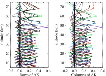
-0.2 0.0 0.2 0.4 0.6 Rows of AK 10 20 30 40 50 60 70 altitude (km) -0.2 0.0 0.2 0.4 0.6 Columns of AK 10 20 30 40 50 60 70 altitude (km)

Fig. 1. Rows (left) and columns (right) of the averaging kernel matrix for a typical MIPAS ozone retrieval. Rows and colomns of the averaging kernel closest to a tangent altitude are highlighted in colors.

per limb sequence from 6 to 68 km (3 km step-width be-tween 6 and 42 km, and at 47, 52, 60, and 68 km). The 3 km step-width is chosen due to the vertical instantaneous field-of-view (FOV) of MIPAS, which is about 3 km, while the across track FOV is about 30 km. The generation of calibrated radiance spectra, the so-called level 1B data, is performed by the European Space Agency (ESA) (Nett et al., 2002). ESA additionally provides vertical profiles of temperature and 6 key species (H2O, O3, HNO3, CH4, N2O, and NO2), the so-called Level 2 product. Furthermore, there are several institutes which have developed retrieval codes to determine trace gases beyond the ESA key species. The ozone distributions used for validation in this paper were derived with the retrieval processor of the Institut f¨ur Meteorologie und Klimaforschung (IMK) and the Instituto de Astrofisica de Andalucia (IAA) (von Clarmann et al., 2003b) and are version V3O O3 7 (publicly available at http://www-imk.fzk.de/asf/ame/envisat-data/).

Validation of a data product involves various self-consistency tests and comparisons (cf. Rodgers, 2000). The characterization of the calibrated radiance spectra has been extensively studied by e.g. Kleinert et al. (2006) and refer-ences therein. The performance of the retrieval processor has been studied in a pre-flight analysis by von Clarmann et al. (2003a), and the characteristics of the retrieved ozone profiles and self-consistency of results have been studied in a sensitivity study by Glatthor et al. (2006). Here we report the final step of validation, which is the comparison of MIPAS ozone profiles to those from other instruments in order to de-tect any potential bias and to verify the predicted precision.

Comparisons of MIPAS IMK-IAA ozone profiles with other satellite instruments have been performed in Wang et al. (2005) and Bracher et al. (2005). In these papers how-ever, older data versions were used and no vertically high

0 2 4 6 8 10 vertical resolution (km) 10 20 30 40 50 60 70 altitude (km)

Fig. 2. Vertical resolution of MIPAS ozone derived from the FWHM of columns (solid) and rows (dashed) of the averaging ker-nel matrix shown in Fig. 1. Dotted lines are for guidance only.

resolved measurements, like ozonesondes, were considered for comparison.

2 MIPAS IMK-IAA ozone data

The ozone data investigated in this paper is produced by the IMK-IAA retrieval processor (von Clarmann et al., 2003b). These data are complementary to the official ESA data prod-uct in a sense that the IMK-IAA retrieval aims at the best possible accuracy in a wide altitude region, while the advan-tage of the ESA data are their better temporal coverage. 2.1 Description

Since launch, MIPAS performed nearly continuous measure-ments until 26 March 2004 in high spectral resolution with a maximum optical path difference of 20 cm. Due to limi-tations in computational resources, at IMK only episodes of particular scientific interest are analyzed which is about 20% of all MIPAS measurements. MIPAS measurements which range from pole to pole (87◦S to 89◦N) are analyzed in quite regular temporal intervals of at least every tenth day. The selected spectral regions used for ozone retrieval, the so-called microwindows, are within the ranges 740–800 cm−1 and 1060–1110 cm−1. For more details see Glatthor et al. (2006). Furthermore, spectra are excluded which are con-taminated with cloud signal. For this, the method described by Spang et al. (2004) is used, however with a more restric-tive cloud index of 4.0.

The retrievals are performed under the assumption of lo-cal thermodynamic equilibrium (LTE), which is valid in the

(4)

0.0 0.2 0.4 0.6 0.8 1.0 error (ppmv) 10 20 30 40 50 60 altitude (km) random noise gain n2o5 los tem h2o systematic spectro ils total 0 5 10 15 20 25 error (%) 10 20 30 40 50 60 altitude (km) random noise gain n2o5 los tem h2o systematic spectro ils total

Fig. 3. Estimated ozone error budget of MIPAS averaged over selected locations (4 seasons, 5 latitude bands, night and day). Left: absolute errors, corresponding to values in volume mixing ratios (vmr). Right: percentage errors.

troposphere and most of the stratosphere in the selected spec-tral regions (Echle et al., 2000). The retrieval is performed on a fixed altitude grid with 1 km step-width up to 44 km, and 2 km step-width above with linear interpolation in altitude between the levels. Since the retrieval grid step-width is finer than the tangent altitude grid (about 3 km, see Sect. 1), reg-ularization is necessary to stabilize the retrieval. Therefore, the iterative retrieval algorithm uses a Tikhonov’s first order smoothing constraint, where the strength of the constraint is based on the number of degrees of freedom (Rodgers, 2000; Steck, 2002). More details on the retrieval setup can also be found in Glatthor et al. (2006).

2.2 MIPAS vertical resolution

The vertical resolution of MIPAS ozone is derived from the averaging kernel matrix (Rodgers, 2000; Steck, 2002). Fig-ure 1 (left) shows the rows of the averaging kernel matrix which gives the contribution of the true ozone values to the retrieved values. The columns of the averaging kernel (Fig. 1, right) gives the response of delta-peak-like perturbations at each altitude. Full-width at half-maximum (FWHM) of both rows and columns of the averaging kernel gives a measure of the vertical resolution of MIPAS ozone retrieval. Figure 2 shows the vertical resolution derived from the averaging ker-nel matrix (Fig. 1). The values are increasing from 3.5 km at 10 km altitude to about 5 km at 42 km, and around 8 km at 60 km altitude. These values are a result of the combination of vertical sampling of measurements (between 3 and 8 km), width of FOV (about 3 km), and regularization.

The oscillating nature of the curve is the result of the fol-lowing: The spacing of the retrieval grid is 1 km whereas the width of the FOV is 3 km, which means that only some re-trieval gridpoints matches a tangent altitude. Generally, this results in a larger diagonal value of the averaging kernel ma-trix (Fig. 1, colored curves) and smaller values in the

ver-tical resolution. Retrieval gridpoints between two tangent alitudes result in smaller diagonal values of the averaging kernel (Fig. 1, black curves) and hence to larger values in vertical resolution.

2.3 MIPAS error budget

Figure 3 shows the MIPAS ozone error budget averaged over selected locations (4 seasons, 5 latitude bands, night and day), which are used in the precision validation (Sect. 5). The estimated total random error (Fig. 3 right, solid black) varies between 4 and 7% between 20 and 52 km corresponding to values in volume mixing ratios (Fig. 3 left, solid black) of 0.15 parts per million by volume (ppmv) and 0.35 ppmv in this altitude region. The percentage errors are slightly in-creasing towards 60 km (12%) and down to 15 km (10%). Below 15 km the percentage errors are rapidly increasing to values in the order of 25% for polar and midlatitude condi-tions or more than 50% for tropical condicondi-tions, where the vmr is small. The error in vmr remains below 0.1 ppmv. The estimated random error is dominated by the instrumen-tal noise above 14 km (Fig. 3 left, solid blue). Below 14 km, the error due to uncertain water vapor concentration becomes dominant (Fig. 3 left, solid beige). The reason for that is the exponentially increasing water vapor with decreasing alti-tude which leads to a dominant water vapor signal in MIPAS spectra. These strong water vapor lines are slightly interfer-ing with ozone lines leadinterfer-ing to a dependence of the retrieved ozone on the pre-retrieved water vapor amount. Also errors due to uncertain gain calibration, N2O5, line-of-sight (LOS) pointing, and temperature contribute noticeably.

The estimated total systematic error (Fig. 3 right, dashed black) is mainly between 4 and 14% (corresponding to 0.1 and 0.8 ppmv, Fig. 3 left, dashed black) with maxima near the ozone maximum and in the lowermost stratosphere and be-low. The error is dominated by uncertainties in spectroscopic

(5)

data (Fig. 3 right, dashed blue). The altitude-dependence of errors due to spectroscopic data is due to the fact that the microwindows used in the retrieval are varying with altitude. Errors caused by uncertainties in the ILS (instrumental line shape) are in the order of 1 to 4% and thus nearly negligible compared to spectroscopic uncertainties.

2.4 MIPAS data versions

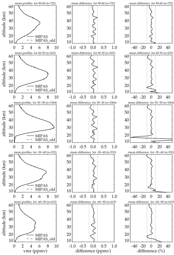
The validation work presented in this paper is based on ozone data of version V3O O3 7 which uses re-processed ESA spectra of version 4.61/4.62. Since there have been several publications with older ozone data (V2 O3 2 and V2 O3 3) based on spectra with versions 4.55 to 4.59, a comparison between the two data sets is performed in the following.

The main difference between version V3O O3 7 and old versions (V2 O3 2 and V2 O3 3) is, besides the different spectra versions, the weaker regularization leading to more degrees of freedom of the retrieved ozone profile and better vertical resolution (Glatthor et al., 2006). Furthermore, the a priori profile is set zero in order to avoid artificial disconti-nuities in the retrieved ozone distributions.

Figure 4 shows the latitude-dependent comparison be-tween the current MIPAS (V3O O3 7) and old MIPAS (V2 O3 2 and V2 O3 3) IMK-IAA profiles. The mean pro-files (Fig. 4, left) are in good agreement showing only little differences. The mean difference (for calculation see Eq. 3) is below ±0.2 ppmv for all altitudes and latitudes (Fig. 4, middle). The mean differences show some similar structures for all latitudes at the same altitudes (e.g., at 17 km, 28 km, and 45 km), which is not surprising, since the regulariza-tion is latitude-independent in both versions. The percent-age mean differences (Fig. 4, right) are below ±5% above 19 km for all latitudes. Remarkable is the large percentage mean difference for tropical conditions (Fig. 4, right, middle row) around 17 km. The mean difference in vmr is similar to other latitudes, but due to the small absolute values, percent-age differences reach 50%. This effect is discussed in more detail in Sect. 5.1 when dealing with ozonesonde comparison at the tropical station Paramaribo. At 14 km a compensation is seen for the differences at 17 km.

Beyond the differences in the retrieval setup, it was found that the different spectra versions (versions 4.55 to 4.59 com-pared to 4.61/62) also cause differences in the retrieval re-sults. In general the mean differences are rather small tween old and new MIPAS ozone data. Only at altitudes be-low 19 km differences can exceed 10%.

3 Validation

3.1 Comparison instruments

MIPAS measurements in high resolution are available from the period July 2002 to March 2004, which are used for com-parison. An overview of geolocations of coincidences with

considered instruments, together with periods of comparison, mean spatial distances, mean temporal differences, and num-bers of coincidences is summarized in Table 1. The different instruments are selected in such a way that all latitudes are covered.

To achieve a large number of correlative measurements, the coincidence criteria for non-satellite instruments are set to: maximum of 6 h in time, maximum of 800 km in dis-tance with a maximum latitudinal disdis-tance of ±4◦. The more stringent latitudinal criterion has proven to be a good choice for all comparisons, since latitudinal variations are in general more pronounced than longitudinal ones.

For the two satellite instruments under consideration a more stringent spatial criterion is used: maximum of 400 km in distance with a maximum latitudinal distance of ±2◦. This still allows for plenty of correlative measurements.

3.2 Strategy and terminology

We use the terminology and formalism as summarized by von Clarmann (2006a,b). In particular, we understand bias is the mean deviation of the measurements from the truth, the relative bias is the mean deviation of profiles measured by two different instruments, and precision is the repro-duceability of a measurement, i.e. the bias-corrected root mean squares difference between MIPAS profiles and the true ozone profiles, all under consideration of effects of fi-nite resolution of the measurements. We further follow the strategy recommended by von Clarmann (2006a) to first de-termine the relative bias between two instruments and to use this for the subsequent precision validation.

In a first step, two co-incident data sets (profiles, aver-aging kernel matrices and covariance matrices), which are given on different altitude grids, need to be made compara-ble. The vertically higher sampled profiles are transformed to the lower sampled altitude grid by

x_h_{= W}∗x_m, (1)

where xhis the high resolved profile from the original mea-surement grid xm, and W∗ is the pseudo-inverse of W (in-terpolation matrix from coarse to fine grid) with W∗W=I (Rodgers, 2000).

There are two possibilities to handle the smoothing error problem. If the altitude resolutions of the co-incident mea-surements are in good approximation equal, the smoothing errors cancel out when the differences between co-incident measurements are calculated and consideration of smoothing errors is necessary neither in bias determination nor in preci-sion validation. This applies to the comparison with MIPAS-B.

If the contrast in altitude resolution is so large that the finer resolved profile can be regarded as an ideal profile, the av-eraging kernel matrix of the coarser resolved profile A can be applied to the finer resolved profile xhin order to adjust

(6)

mean profiles for 90-60 (n=722) 0 2 4 6 8 10 10 20 30 40 50 60 altitude (km) MIPAS MIPAS_old

mean difference for 90-60 (n=722)

-1.0 -0.5 0.0 0.5 1.0 10 20 30 40 50

60 mean difference for 90-60 (n=722)

-40 -20 0 20 40 10 20 30 40 50 60

mean profiles for 60-30 (n=623)

0 2 4 6 8 10 10 20 30 40 50 60 altitude (km) MIPAS MIPAS_old

-1.0 -0.5 0.0 0.5 1.0 10 20 30 40 50

-40 -20 0 20 40 10 20 30 40 50 60

mean profiles for 30--30 (n=1064)

mean difference for 30--30 (n=1064)

-1.0 -0.5 0.0 0.5 1.0 10 20 30 40 50

60 mean difference for 30--30 (n=1064)

-40 -20 0 20 40 10 20 30 40 50 60

mean profiles for -30--60 (n=532)

mean difference for -30--60 (n=532)

-1.0 -0.5 0.0 0.5 1.0 10 20 30 40 50

60 mean difference for -30--60 (n=532)

-40 -20 0 20 40 10 20 30 40 50 60

0 2 4 6 8 10 vmr (ppmv) 10 20 30 40 50 60 altitude (km) MIPAS MIPAS_old

-1.0 -0.5 0.0 0.5 1.0 difference (ppmv) 10 20 30 40 50

-40 -20 0 20 40 difference (%) 10 20 30 40 50 60

Fig. 4. Comparison of MIPAS version V3O O3 7 and older versions (V2 O3 2 and V2 O3 3, MIPAS old) ozone profiles for 5 latitude bins. From top to bottom (number of coincidences in brackets): 90◦N to 60◦N (722), 60◦N to 30◦N (623), 30◦N to 30◦S (1064), 30◦S to 60◦S (532), and 60◦S to 90◦S (615). From left to right: Mean ozone profiles, mean difference, and percentage mean difference. Dotted lines are for guidance only.

(7)

Table 1. Geolocations of considered instruments together with period of comparison, mean spatial distance 1_d, mean temporal difference

1t, and number of comparison pairs.

Instrument lat/lon period 1d 1t coinc.

location (type) [deg] [km] [h] [#] Ny- ˚Alesund (lidar) 78.9/11.9 10.2002–03.2003 460 2.6 362 Alomar (lidar) 69.3/16.0 09.2002–03.2004 456 2.6 108 Sodankyla (sonde) 67.8/26.6 08.2002–03.2004 456 2.8 163 Kiruna (FTIR) 67.8/20.4 09.2002–03.2004 498 1.9 498 Kiruna (microwave) 67.8/20.4 11.2002–12.2003 427 2.8 412 Hohenpeissenberg (lidar) 47.8/11.0 09.2002–03.2004 457 1.6 133 Hohenpeissenberg (sonde) 47.8/11.0 07.2002–03.2004 492 4.0 130 Zugspitze (microwave) 47.4/11.0 02.2003–07.2003 512 2.3 77 Izana (sonde) 28.5/–16.3 07.2002–03.2004 541 0.4 50 Izana (FTIR) 28.5/–16.3 09.2002–03.2004 519 2.8 189 Paramaribo (sonde) 5.8/–55.2 07.2002–03.2004 343 1.3 19 Belgrano (sonde) –77.8/–34.6 07.2002–03.2004 393 2.8 127 MIPAS-B (balloon) campaigns 09.2002–07.2003 274 2.2 9 HALOE (satellite) globally 09.2002–02.2004 227 3.8 333 POAM (satellite) N + S poles 09.2002–03.2004 214 3.3 674

it to the altitude resolution of the coarser resolved profile (Rodgers, 2000; Rodgers and Connor, 2003):

x= xa+ A(xh− xa), (2)

where xa is the a priori profile of the coarser resolved pro-file. In case of MIPAS, where xais zero, Eq. (2) simplifies to x=Axh. After this transformation, the smoothing char-acteristics have not to be considered any further. In case of ground-based sounding by microwave and FTIR instruments, their averaging kernels are used to smooth the MIPAS pro-files, whereas the higher resolved lidar, ozonesonde, HALOE and POAM profiles are smoothed by the MIPAS averaging kernels. Residual smoothing error differences not accounted for correctly by the approaches above because the assump-tions made may hold only in approximation, are discussed in von Clarmann and Grabowski (2007).

For bias determination and precision validation we follow the strategy proposed by von Clarmann (2006a). In particu-lar we perform validation of ozone mixing ratios at discrete altitudes individually instead of profile validation (Rodgers, 2000; Migliorini et al., 2004), in order not to depend on co-variance information between the altitudes. Since the true at-mospheric state is not known, we can only estimate the rela-tive bias ˘bdiff(or mean difference) between two datasets from a sample of K co-incident pairs of measurements, which is

˘b_diff= PK

k=1( ˆxMIPAS;k− ˆxref;k)

K , (3)

where ˆx_MIPAS;k are the ozone profiles retrieved by MIPAS, and ˆx_ref;k are the co-incident profiles measured by the ref-erence instrument. The statistical uncertainty of the bias

˘

σbias;n, at altitude gridpoint n is estimated as

˘

σbias;n=

s PK

k=1( ˆxMIPAS;n,k− ˆxref;n,k− ˘bdiff;n)2

K(K − 1) , (4)

for samples large enough to disregard t-statistics (Gosset, 1908). As pointed out by von Clarmann (2006a), this assess-ment does not need any error estimates of ˆx_MIPASor ˆx_ref. For percentage multiplicative bias estimates we use the percent-age mean difference rather than the mean percentpercent-age differ-ence.

With the relative bias between two instruments available, the precision at altitude gridpoint n is validated by altitude-wise testing of the de-biased mean squares difference of the co-incident measurements against the ex ante estimate of the variance of the difference σ_diff;n,k2 in a χ2sense:

χ2= PK

k=1( ˆxMIPAS;n,k− ˆxref;n,k− ˘bdiff;n)2/K

σ_diff;n,k2 . (5)

The ex ante estimate of the variance of random error of the difference σ_diff2 (or in short form: estimated combined ran-dom error) includes the following additive components: the estimated random error variance of MIPAS ozone; the esti-mated random error variance of the ozone abundance mea-sured with the reference instrument; the variance represent-ing the expected difference due to less than perfect coinci-dence. In our application no smoothing error of the differ-ence has to be considered here, because of application of Eq. (2) whenever relevant.

The error due to less than perfect coincidence (or spatial-temporal mismatch) is derived from ECMWF (European

(8)

Centre for Medium-Range Weather Forecasts) ozone distri-butions and is calculated as follows:

σ_mm;n,k2 =(δxt;n1t;k)2+(δxlat;n1lat;k)2+(δxlon;n1lon;k)2. (6)

δxlat;n is the difference in ozone at altitude n between two

different latitude points, divided by the distance in latitude direction, and averaged over a longitudinal bin of 10 degrees.

δxlon;nand δxt;n are defined like δxlat;nbut for longitudinal

and temporal differences. 1lat;k, 1lon;k, and 1t;k are the ac-tual differences in latitude, longitude, and time for the com-parison pair k.

4 Bias determination

4.1 Comparisons with ground-based instruments 4.1.1 Lidar data

Comparison measurements are performed with stratospheric ozone lidar systems. The technique used is the so-called Differential Absorption Lidar (DIAL) (see, e.g. Godin et al., 1999). Ozone profiles are usually measured in reliable qual-ity between 10 and 45 km altitude. The data was taken from the NILU (Norwegian Institute for Air Research) server for the stations at Hohenpeissenberg, Alomar, and Ny- ˚Alesund. Since the ozone concentration is given in number densities, the values are transformed into volume mixing ratios for proper comparison with MIPAS results.

Measurements at Hohenpeissenberg (47.8◦N, 11.0◦E) were available for the entire comparison period. The com-parison is shown in Fig. 5 (top), where 133 comcom-parison pairs were found. The mean profiles (Fig. 5, left) show good agreement with mean differences (Fig. 5, middle) be-low ±0.2 ppmv up to 30 km altitude, and reaching about 0.5 ppmv at 38 km. The percentage mean differences (Fig. 5, right) are within ±10% except at 16 km, where the percent-age mean difference reaches 15%. The rather large positive difference around 38 km is likely due to a negative bias in the lidar data, which was found in comparison with SAGE II (W. Steinbrecht, personal communication, 2006).

Measurements at Alomar (69.3◦N, 16.0◦E) were avail-able for the entire comparison period with 108 comparison pairs. The mean profiles (Fig. 5, middle left) agree very well up to 44 km with mean differences (Fig. 5, middle) below ±0.3 ppmv. The large differences at the upper end of the al-titude range can be explained by the rather large uncertainty in lidar data there. The percentage mean difference (Fig. 5, right) is below ±10% between 13 and 44 km. At very low altitudes, mean differences become negative with values of up to –20%.

Measurements at Ny- ˚Alesund (78.9◦N, 11.9◦E) (Stein-brecht et al., 1999) were available between October 2002 and March 2003 resulting in 362 comparison pairs. The mean profiles (Fig. 5, bottom left) show good agreement up to

36 km with mean differences below about ±0.2 ppmv (Fig. 5, middle). Above 36 km mean differences between MIPAS and Ny- ˚Alesund lidar reach values of about −0.5 ppmv. Above 44 km the lidar values become again unreasonably large. The percentage mean differences (Fig. 5, right) are be-low ±10% between 17 and 43 km. At 13 km the difference reaches +15%.

4.1.2 FTIR data

Measurements are performed with ground-based Fourier transform spectrometers in the infrared region (FTIR). The spectrometers are directed to the sun measuring atmospheric absorption spectra. For ozone, a broad microwindow around 1000 cm−1and two narrow ones around 780 cm−1are used. The number of independent pieces of information (or degrees of freedom) is around 5, leading to a vertical resolution of about 6–7 km, depending on altitude and atmospheric situa-tion.

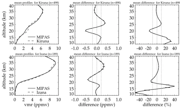
Ozone profiles at Kiruna (67.8◦N, 20.4◦E) (Kopp et al., 2002.) were available for the entire comparison period. Fig-ure 6 (top left) shows the comparison between MIPAS and FTIR mean ozone profiles. The agreement is reasonable ex-cept a pronounced discrepancy between 18 and 28 km where the mean difference exceeds the uncertainty of the mean dif-ference by far. This is attributed to specific choice of the FTIR a priori profile, which is only corrected in part by ap-plication of Eq. (2) due to non-linearities in the ground-based retrieval. Percentage mean differences are below ±10% (Fig. 6, right) above 22 km.

In addition to profile comparison, partial zenith column densities of ozone between 10 and 40 km have been ana-lyzed. The agreement between MIPAS and FTIR (Kiruna) is very good (see Table 2) with a percentage mean difference of 0.4% which is close to the estimated error of the mean differ-ence (0.3%). This supports our explanation that differdiffer-ences in the profile comparison are caused by residual altitude res-olution and a priori differences as discussed above.

Also Izana (28.2◦N, 16.3◦W) FTIR ozone profiles (Schneider et al., 2004) were available from September 2002 until March 2004. The mean profiles (Fig. 6, bottom left) show good agreement where the mean differences are less than ±0.4 ppmv (Fig. 6, middle). The percentage mean differences are below ±15% above 18 km altitude (Fig. 6, right). The large percentage mean difference around 17 km can partly be attributed to the spatial coincidence criteria. More restrictive criteria (600 km in distance and 3◦ in lat-itude) reduce the percentage mean difference from 40% to 20% (not shown).

Like in the Kiruna case, partial columns of ozone between 10 and 40 km have been compared in addition. The agree-ment between MIPAS and FTIR (Izana) is again very good (see Table 2) with a percentage mean difference of −0.4%.

(9)

mean profiles for Hohenp (n=133) 0 2 4 6 8 10 15 20 25 30 35 40 45 altitude (km) MIPAS Hohenp

mean difference for Hohenp (n=133)

-1.0 -0.5 0.0 0.5 1.0 10 15 20 25 30 35 40

45 mean difference for Hohenp (n=133)

-40 -20 0 20 40 10 15 20 25 30 35 40 45

mean profiles for Alomar (n=108)

0 2 4 6 8 10 15 20 25 30 35 40 45 altitude (km) MIPAS Alomar

mean difference for Alomar (n=108)

-1.0 -0.5 0.0 0.5 1.0 10 15 20 25 30 35 40

45 mean difference for Alomar (n=108)

-40 -20 0 20 40 10 15 20 25 30 35 40 45

mean profiles for NyAlesund (n=362)

0 2 4 6 8 vmr (ppmv) 10 15 20 25 30 35 40 45 altitude (km) MIPAS NyAlesund

mean difference for NyAlesund (n=362)

-1.0 -0.5 0.0 0.5 1.0 difference (ppmv) 10 15 20 25 30 35 40

45 mean difference for NyAlesund (n=362)

-40 -20 0 20 40 difference (%) 10 15 20 25 30 35 40 45

Fig. 5. Comparison of MIPAS and lidar ozone profiles. From top to bottom (number of coincidences in brackets): Hohenpeissenberg (133), Alomar (108), and Ny- ˚Alesund (362). From left to right: MIPAS (solid) and lidar (dashed) mean profiles, mean difference (solid) between MIPAS and lidar with uncertainty of the mean (error bars), and percentage mean difference (solid) between MIPAS and lidar with uncertainty of the mean (error bars). Dotted lines are for guidance only.

Table 2. Comparison of MIPAS and FTIR partial zenith column densities between 10 and 40 km altitude. Entries in the table from left to right are: station, number of comparison pairs, mean partial columns of MIPAS and FTIR, mean difference, and uncertainty of the mean. Values are given in units of 1020m−2.

Station N MIPAS FTIR b˘diff σ˘bias

Kiruna 498 745.8 743.1 2.7 (0.4%) 2.1 (0.3%) Izana 189 676.3 679.3 –3.0 (–0.4%) 2.0 (0.3%)

4.1.3 Microwave data

Two ground-based microwave radiometers were used for MIPAS validation, the 195–224 GHz Kiruna microwave ra-diometer KIMRA at IRF Kiruna (Raffalski et al., 2005) and the 268–280 GHz millimeter wave radiometer MIRA 2 of

IMK Karlsruhe (Kopp et al., 2002.). The retrieved ozone pro-files of both instruments have a vertical resolution of about 6– 8 km in the lower stratosphere degrading to more than 15 km in the lower mesosphere. The degrees of freedom amount to about 4 for measurements taken during good weather condi-tions.

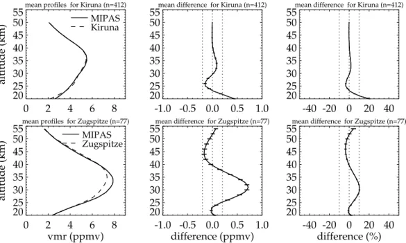
Measurements from Kiruna (67.8◦N, 20.4◦E) were avail-able from November 2002 until December 2003. Mean pro-files of MIPAS and KIMRA are displayed in Fig. 7 (top left) showing very good agreement above 22 km with mean dif-ferences below ±0.2 ppmv (Fig. 7, middle). The nearly per-fect agreement above 40 km is due to the strong influence of the microwave regularization at these altitudes since the measurement response is rather low. The smoothed MIPAS results are forced to the microwave a priori profile. Percent-age mean differences (Fig. 7, right) are below ±5% above 22 km. In both, mean absolute and percentage mean differ-ence, no indication of a systematic bias in MIPAS ozone is noticeable.

(10)

mean profiles for Kiruna (n=498) 0 2 4 6 8 10 10 15 20 25 30 35 40 altitude (km) MIPAS Kiruna

mean difference for Kiruna (n=498)

-1.0 -0.5 0.0 0.5 1.0 10 15 20 25 30 35

40 mean difference for Kiruna (n=498)

-40 -20 0 20 40 10 15 20 25 30 35 40

mean profiles for Izana (n=189)

0 2 4 6 8 10 vmr (ppmv) 10 15 20 25 30 35 40 altitude (km) MIPAS Izana

mean difference for Izana (n=189)

-1.0 -0.5 0.0 0.5 1.0 difference (ppmv) 10 15 20 25 30 35

40 mean difference for Izana (n=189)

-40 -20 0 20 40 difference (%) 10 15 20 25 30 35 40

Fig. 6. Comparison of MIPAS and FTIR ozone profiles. From top to bottom (number of coincidences in brackets): Kiruna (498) and Izana (189). From left to right: see Fig. 5.

Table 3. Comparison of MIPAS and microwave partial zenith col-umn densities between 20 and 60 km altitude. Entries in the table from left to right are: station, number of comparison pairs, mean partial columns of MIPAS and microwave (MW), mean difference, and uncertainty of the mean. Values are given in units of 1020m−2.

Station N MIPAS MW b˘_diff σ˘_bias

Kiruna 412 404.0 403.7 0.3 (0.1%) 2.6 (0.6%)

Zugspitze 77 589.6 573.8 15.8 (2.7%) 3.6 (0.6%)

In addition to profile comparison, partial columns of ozone between 20 and 60 km have been analyzed. The agreement between MIPAS and microwave (Kiruna) is very good (see Table 3) with a percentage mean difference of 0.1% which is below the estimated error of the mean difference (0.6%).

Ozone profiles from Zugspitze (47.4◦N, 11.0◦E) were available for the MIRA campaign between February and July 2003. The comparison is shown in Fig. 7. There is good agreement below 25 km and above 38 km with mean differ-ences (Fig. 7, middle) smaller than ±0.2 ppmv. In the ozone maximum, MIPAS mean values are larger than MIRA by up to 0.7 ppmv. The related percentage differences (Fig. 7, right) remain below ±10%. The larger differences at the up-per end of the comparison region can be attributed to diurnal variations in ozone. Microwave measurements at Zugspitze have been performed mainly during daytime, whereas MI-PAS measurements also have significant nighttime contribu-tions with enhanced ozone values above about 50 km.

Table 4. Ozone sonde types and manufacturers for different sta-tions. Abbreviations: ECC (Electrochemical Concentration Cell), BM (Brewer Mast).

Station Type Manufacturer

Sodankyla ECC both SPC-6A and ENSCI-Z Hohenpeissenberg BM –

Izana ECC SPC-6A Paramaribo ECC SPC-6A

Belgrano ECC both SPC-6A and ENSCI-Z

Like in the Kiruna case, partial columns of ozone between 20 and 60 km have been compared in addition. The agree-ment between MIPAS and microwave (Zugspitze) is not as good as for the Kiruna station (see Table 3) with a percent-age mean difference of 2.7%. However, this is not surprising considering the 10% difference in the mean ozone profiles near the ozone maximum.

4.2 Comparisons with balloon-borne instruments 4.2.1 Ozonesondes

Measurements are performed in situ with ozonesondes of the types electrochemical concentration cell (ECC) and Brewer-Mast (BM) on small balloons (see Table 4). Ozone profiles are usually measured with low random error and high vertical resolution (Smit and Straeter, 2004) from the Earth’s surface

(11)

mean profiles for Kiruna (n=412) 0 2 4 6 8 20 25 30 35 40 45 50 55 altitude (km) MIPAS Kiruna

mean difference for Kiruna (n=412)

-1.0 -0.5 0.0 0.5 1.0 20 25 30 35 40 45 50

55 mean difference for Kiruna (n=412)

-40 -20 0 20 40 20 25 30 35 40 45 50 55

mean profiles for Zugspitze (n=77)

0 2 4 6 8 vmr (ppmv) 20 25 30 35 40 45 50 55 altitude (km) MIPAS Zugspitze

mean difference for Zugspitze (n=77)

-1.0 -0.5 0.0 0.5 1.0 difference (ppmv) 20 25 30 35 40 45 50

55 mean difference for Zugspitze (n=77)

-40 -20 0 20 40 difference (%) 20 25 30 35 40 45 50 55

Fig. 7. Comparison of MIPAS and microwave ozone profiles. From top to bottom (number of coincidences in brackets): Kiruna (412) and Zugspitze (77). From left to right: see Fig. 5.

up to the mid stratosphere (about 32 km). Since ozone is measured in partial pressure, the values can be easily trans-formed into vmrs. The data was taken from the NILU (Nor-wegian Institute for Air Research) server except for Izana.

Measurements at Sodankyla (67.4◦N, 26.6◦E) were avail-able for the entire measurement time of MIPAS. The com-parison is shown in Fig. 8 (top), where the mean profiles (left) agree very well. The mean difference (middle) is below ±0.2 ppmv for the complete altitude range. Also the percent-age mean difference (Fig. 8, right) is very small and exceeds ±6% difference only around 15 km and below 10 km alti-tude.

The comparison with measurements at Hohenpeissenberg (47.8◦N, 11.0◦E) is shown in Fig. 8 (second from top). The mean difference (middle) is increasing with altitude above 25 km and reaching values larger than +0.5 ppmv. The percentage mean difference reaches values of +20% below 16 km altitude. At higher altitudes the difference is contin-uously increasing and reaching +10% at 30 km. A positive mean difference is noticeable in both troposphere and strato-sphere.

Izana (28.5◦N, 16.3◦W) measurements are compared with MIPAS and results are shown in Fig. 8 (third from top). The mean difference (Fig. 8, middle) is increasing with alti-tude above 21 km and reaches +0.5 ppmv at 28 km altialti-tude. The percentage mean difference is below ±20% in the tro-posphere and below 10% in the lower stratosphere. Similar to the Hohenpeissenberg comparison, a positive mean differ-ence between MIPAS and ozonesonde is noticeable.

Paramaribo (5.8◦N, 55.2◦W) measurements are also available for the entire comparison time interval. However, only 19 coincidences were found for this period. The mean profiles are displayed in Fig. 8 (second from bottom, left). The mean differences (middle) are below ±0.3 ppmv be-low 24 km altitude. Above 24 km altitude the differences are continuously increasing towards −0.7 ppmv. This is in contradiction to the higher MIPAS ozone mixing ratios at Hohenpeissenberg and Izana. A hint that these systematic differences are not a problem of MIPAS but of the different ozonesondes is given in Smit and Straeter (2004), who report biases between different ozonesonde systems of up to 10%.

At 17 km MIPAS is underestimating ozone values consid-erably by about 0.3 ppmv leading to even a negative mixing ratio in the mean. In the IMK-IAA MIPAS retrieval negative mixing ratios are not suppressed. While these are physically meaningless, a positivity constraint such as the retrieval of the logarithms of vmr instead of vmr adds complication to the statistical analysis of results and thus has not been ap-plied to the current retrievals.

Investigation of the Paramaribo case has shown, that appli-cation of averaging kernels has basically no influence on the difference between MIPAS and sonde profiles, which means that the smoothing error of the MIPAS retrieval is not re-sponsible for the negative values around 17 km. Dependence on temperature and water vapor was found negligibly small. However, in a revision of the MIPAS retrieval baseline, one suspicious microwindow around 742 cm−1has been detected to be used around 17 km tangent altitude. Disregard of this microwindow decreases the difference between ozonesonde

(12)

mean profiles for Sodankyla (n=163) 0 2 4 6 8 10 12 10 15 20 25 30 altitude (km) MIPAS Sodankyla

mean difference for Sodankyla (n=163)

-1.0 -0.5 0.0 0.5 1.0 10 15 20 25 30

mean difference for Sodankyla (n=163)

-40 -20 0 20 40 10 15 20 25 30

mean profiles for Hohenp (n=130)

0 2 4 6 8 10 12 10 15 20 25 30 altitude (km) MIPAS Hohenp

-1.0 -0.5 0.0 0.5 1.0 10 15 20 25 30

-40 -20 0 20 40 10 15 20 25 30

mean profiles for Izana (n=50)

0 2 4 6 8 10 12 10 15 20 25 30 altitude (km) MIPAS Izana

-1.0 -0.5 0.0 0.5 1.0 10 15 20 25 30

-40 -20 0 20 40 10 15 20 25 30

mean profiles for Paramaribo (n=19)

0 2 4 6 8 10 12 10 15 20 25 30 altitude (km) MIPAS Paramaribo

mean difference for Paramaribo (n=19)

-1.0 -0.5 0.0 0.5 1.0 10 15 20 25 30

mean difference for Paramaribo (n=19)

-40 -20 0 20 40 10 15 20 25 30

mean profiles for Belgrano (n=127)

0 2 4 6 8 10 12 vmr (ppmv) 10 15 20 25 30 altitude (km) MIPAS Belgrano

mean difference for Belgrano (n=127)

-1.0 -0.5 0.0 0.5 1.0 difference (ppmv) 10 15 20 25 30

mean difference for Belgrano (n=127)

-40 -20 0 20 40 difference (%) 10 15 20 25 30

Fig. 8. Comparison of MIPAS and ozonesonde profiles. From top to bottom (number of coincidences in brackets): Sodankyla (163), Hohenpeissenberg (130), Izana (50), Paramaribo (19), and Belgrano (127). From left to right: see Fig. 5.

(13)

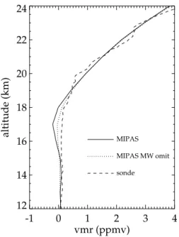
-1 0 1 2 3 4 vmr (ppmv) 12 14 16 18 20 22 24 altitude (km) _MIPAS MIPAS MW omit sonde

Fig. 9. Comparison of MIPAS and ozonesonde (Paramaribo) pro-files for 6 February 2003. Omitting one microwindow at one alti-tude leads to better MIPAS result (dotted line).

and MIPAS (see Fig. 9) but does not fully remove it (dot-ted line in Fig. 9). This microwindow seems to be particu-larly sensitive to residual cloud signal in the spectra caused by e.g. very thin cirrus clouds undetected by the cloud filter-ing procedure. Negative ozone mixfilter-ing values were retrieved by MIPAS particularly when the actual cloud index was low but still higher than the threshold used by the cloud detection algorithm. An estimation of the retrieval error due to cirrus clouds has been done in Glatthor et al. (2006), which shows a considerable increase of the ozone error. The negative ten-dency of the ozone values are not yet understood and further investigations are necessary.

The comparison with measurements at Belgrano (77.8◦S, 34.6◦W) is shown in Fig. 8 (bottom). The mean profiles (Fig. 8, left) agree well, with a rather positive mean differ-ence. In absolute values this is mostly pronounced above 20 km (Fig. 8, middle). The percentage mean difference (Fig. 8, right) is below ±20% above 17 km altitude. Below 17 km the percentage mean difference reaches 30% but the mean absolute differences are below 0.2 ppmv.

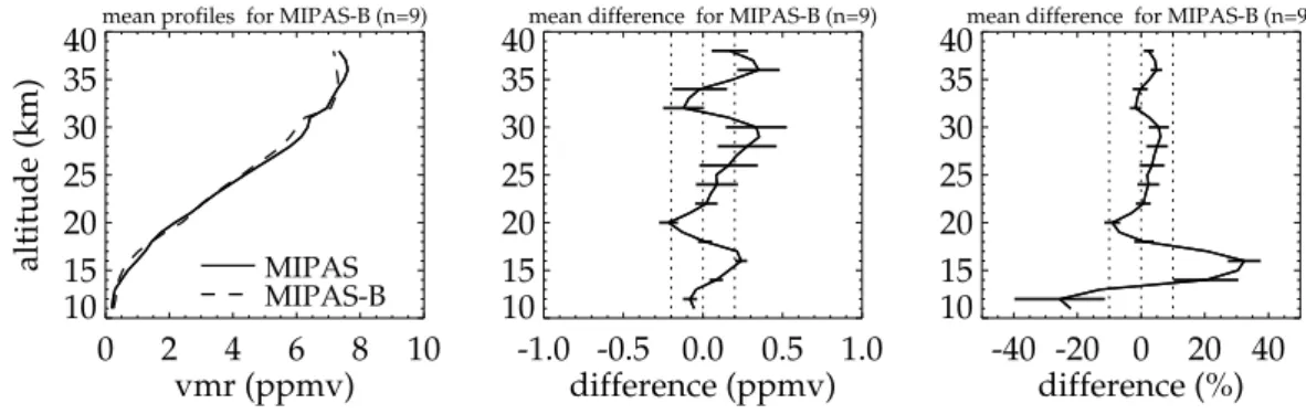
4.2.2 MIPAS-B

MIPAS-B (Friedl-Vallon et al., 2004) is the balloon-borne version of MIPAS measuring the atmospheric emission in a limb viewing mode. The spectral resolution (0.034 cm−1) and the vertical resolution (2–3 km) is similar to the space-borne MIPAS. MIPAS-B measurements performed near Aire sur l’Adour (24 September 2002, Envisat validation cam-paign) and Kiruna (20/21 March and 3 July 2003) are com-pared to those made by MIPAS-Envisat.

Figure 10 shows the comparison of MIPAS-Envisat and MIPAS-B ozone measurements. The mean profiles (Fig. 10, left) agree very well with mean differences below about ±0.3 ppmv for the complete altitude range. Percentage mean differences are within ±10% above 17 km. Around 15 km, the percentage mean difference is positive, which has already been detected in comparison with ozonesondes. The larger differences can partly be attributed to air parcels viewed by the instruments which are inside or at the edge of the vortex.

4.3 Comparisons with satellite instruments

4.3.1 HALOE

HALOE (Halogen Occultation Experiment) is a solar occul-tation instrument (Russell III et al., 1993) on board the Upper Atmosphere Research Satellite launched in September 1991. It measured ozone during sunrise and sunset atmospheric conditions. Due to the limb-viewing geometry a good verti-cal resolution (about 2.3 km) was achieved, which is slightly better than that of MIPAS. The measurements were made in the mid IR, at 9.6 µm, which is partly the same band used in MIPAS retrievals. For the comparison, HALOE version 19 data is used.

Figure 11 shows the global comparison between MIPAS and HALOE. For nearly all altitudes, we see a positive mean difference (Fig. 11, middle) between MIPAS and HALOE with values up to 0.6 ppmv at 28 km and 44 km. The positive mean differences are attributed to the use of different spec-troscopic databases. HALOE uses line strengths which are increased by 5% compared to HITRAN 92 leading to smaller mean ozone values (Br¨uhl et al., 1996; Randall et al., 2003). This is confirmed by a bias in the percentage mean differ-ence (Fig. 11, right) between roughly 0 and 10%. Since the microwindows used for MIPAS vary with altitude, it is expected that the bias also varies with altitude. Below 15 km, mean percentage differences become larger, which has already been detected in comparisons to ozonesondes (see Sect. 4.2.1).

The pronounced structure at around 18 km (see Fig. 11, middle) is attributed to the residual cloud signal problem in the suspicious microwindow used in the MIPAS retrieval, which has already been discussed in the context of the comparison with Paramaribo ozonesonde measurements (see Sect. 4.2.1). Too small MIPAS values do not only appear in the tropical region, but at all latitudes (Fig. 11). This indi-cates that not only cirrus, but also polar stratospheric clouds (PSCs) could be involved.

The other sharp structure at around 32 km is caused by a discontinuity in the MIPAS background continuum emis-sion, which is set zero above this altitude but fitted below (von Clarmann et al., 2003b). Glatthor et al. (2006) have found by sensitivity studies that this leads to compensation effects which introduce a structure in MIPAS ozone profiles

(14)

mean profiles for MIPAS-B (n=9) 0 2 4 6 8 10 vmr (ppmv) 10 15 20 25 30 35 40 altitude (km) MIPAS MIPAS-B

mean difference for MIPAS-B (n=9)

-1.0 -0.5 0.0 0.5 1.0 difference (ppmv) 10 15 20 25 30 35

40 mean difference for MIPAS-B (n=9)

-40 -20 0 20 40 difference (%) 10 15 20 25 30 35 40

Fig. 10. Comparison of MIPAS-Envisat and MIPAS-B ozone profiles (9 coincidences). From left to right: see Fig. 5.

around 32 km. A revision of the retrieval strategy for the at-mospheric continuum emission is under way.

4.3.2 POAM III

Polar Ozone and Aerosol Measurement III (POAM III, Lucke et al., 1999; Lumpe et al., 2002) on board the SPOT-4 satellite was launched in March 1998. POAM III uses, like HALOE, the solar occultation technique for measuring the vertical distribution of ozone during sunrise and sunset. The spectral region used for ozone measurements lies, unlike MI-PAS and HALOE, in the visible region at 603 nm. The verti-cal resolution (Randall et al., 2003) in the stratosphere (15 to 50 km altitude) is 1 km, reaching 5 km at 5 km altitude, and 2.5 km at 60 km altitude. For the comparison, POAM version 4 data is used.

Due to the given orbit of SPOT-4, there are no measure-ments between about 50◦N and 50◦S available. Together with the coincidence criteria (Sect. 3.1) only comparisons polewards of 50◦N and 60◦S have been found leading to 674 comparison pairs.

Figure 12 shows the comparison between MIPAS and POAM correlative measurements divided into northern and southern polar regions. The mean profiles (Fig. 12, left) of MIPAS and POAM agree well. At 32 km a slight negative kink in the mean MIPAS results is visible (especially in the southern polar region) but not present in POAM. In the com-parison with HALOE this feature has already been discussed and is due to the strategy of atmospheric continuum retrieval. Since this feature seems to be more pronounced in the south-ern polar region suggests that very thin PSCs may have an influence on the ozone retrieval due to upward error propa-gation. With a vertical FOV slightly larger than 3 km, the suggestion above becomes more likely.

When considering the entire altitude range, there is no ob-vious bias of any sign visible (Fig. 12, middle), leading to mean differences mainly below ±0.2 ppmv. The percentage mean differences (Fig. 12, right) are below ±10% for all alti-tudes and both polar regions. Below 20 km, a similar feature like in the HALOE comparison is visible, however less pro-nounced, which is due to the given latitude region.

4.4 Summary

In the previous sections, MIPAS ozone data have been com-pared to single instruments which give findings for specific locations and altitudes. In most altitudes and latitude bands, MIPAS ozone agrees well with the comparison instruments. Two problems have been identified: First, MIPAS ozone has a systematic negative kink around 32 km. This is explained by the treatment of atmospheric continuum emission in the retrieval (c.f. Sect. 4.3.1), which is forced to zero above this altitude. The transition will be moved to higher altitudes where the actual continuum signal can be expected to be zero. Second, around 18 km MIPAS ozone tends to low val-ues. At least part of this problem has been solved and can be attributed to a particular microwindow used at these altitudes which will be removed in future versions.

In addition to the local and latitude band-wise investiga-tion a comprehensive global comparison between MIPAS ozone and all other validation data from the different instru-ment types (lidar, FTIR, microwave, ozonesonde, MIPAS-B, HALOE, and POAM) is performed. The mean differences (Fig. 13, left) are within ±0.5 ppmv at all altitudes showing very good agreement between MIPAS and the comparison instruments. The mean differences have a slight positive ten-dency particularly in the lower stratosphere with values be-tween −0.1 and 0.5 ppmv. FTIR values around 20 km seem to be too high compared to the other instruments. Mean dif-ferences below 18 km show values between −0.1 ppmv and 0.2 ppmv. Around 15 km altitude, MIPAS ozone is higher compared to most other instruments which is likely a com-pensation for the negative kink above.

The percentage mean differences (Fig. 13, right) are within ±10% above 18 km with very few exceptions. This is mainly within the expected systematic errors of MIPAS which are in the order of 5 to 10% (see Fig. 3). The large mean differ-ences detected in specific latitude bands around 18 km are below −5% compared to most instrument types and are of less importance on a global scale. Below 17 km the percent-age mean differences become larger with a positive tendency compared to most instrument types with values between −20

(15)

mean profiles for 90-60 (n=69) 0 2 4 6 8 10 10 20 30 40 50 altitude (km) MIPAS HALOE

-1.0 -0.5 0.0 0.5 1.0 10

20 30 40

-40 -20 0 20 40 10 20 30 40 50

mean profiles for 60-30 (n=67)

0 2 4 6 8 10 10 20 30 40 50 altitude (km) MIPAS HALOE

-1.0 -0.5 0.0 0.5 1.0 10

20 30 40

-40 -20 0 20 40 10 20 30 40 50

mean profiles for 30--30 (n=49)

mean difference for 30--30 (n=49)

-1.0 -0.5 0.0 0.5 1.0 10

20 30 40

50 mean difference for 30--30 (n=49)

-40 -20 0 20 40 10 20 30 40 50

-1.0 -0.5 0.0 0.5 1.0 10

20 30 40

-40 -20 0 20 40 10 20 30 40 50

0 2 4 6 8 10 vmr (ppmv) 10 20 30 40 50 altitude (km) MIPAS HALOE

-1.0 -0.5 0.0 0.5 1.0 difference (ppmv) 10 20 30 40

-40 -20 0 20 40 difference (%) 10 20 30 40 50

Fig. 11. Comparison of MIPAS and HALOE ozone profiles for 5 latitude bins. From top to bottom (number of coincidences in brackets): 90◦N to 60◦N (69), 60◦N to 30◦N (67), 30◦N to 30◦S (49), 30◦S to 60◦S (54), and 60◦S to 90◦S (94). From left to right: see Fig. 5.

(16)

mean profiles for 90-50 (n=347) 0 1 2 3 4 5 6 7 10 20 30 40 50 60 altitude (km) MIPAS POAM

-1.0 -0.5 0.0 0.5 1.0 10 20 30 40 50

-40 -20 0 20 40 10 20 30 40 50 60

0 1 2 3 4 5 6 7 vmr (ppmv) 10 20 30 40 50 60 altitude (km) MIPAS POAM

-1.0 -0.5 0.0 0.5 1.0 difference (ppmv) 10 20 30 40 50

-40 -20 0 20 40 difference (%) 10 20 30 40 50 60

Fig. 12. Comparison of MIPAS and POAM ozone profiles for 2 latitude bins. From top to bottom (number of coincidences in brackets): 90◦N to 60◦N (347) and 60◦S to 90◦S (327). From left to right: see Fig. 5.

-1.0 -0.5 0.0 0.5 1.0 difference (ppmv) 10 20 30 40 50 60 altitude (km) -40 -20 0 20 40 difference (%) 10 20 30 40 50 60 altitude (km)

Fig. 13. Comprehensive global comparison of ozone from MIPAS with HALOE (333 comparison pairs, solid blue), POAM (674, dashed blue), lidar (603, solid red), FTIR (687, dashed red), microwave (489, dotted red), ozonesonde (489, solid green), and MIPAS-B (9, dashed green). Left: mean difference between MIPAS and others with uncertainty of the mean (error bars), right: percentage mean difference between MIPAS and others with uncertainty of the mean (error bars). Dotted lines are for guidance only.

and 30%. Here, the mean differences exceed the estimated systematic errors of MIPAS. But considering that the com-parison instruments also have biases, the found mean differ-ences are of reasonable size and should not be overstressed.

5 Precision validation

In this section the estimated random error of the difference is compared with the bias-corrected root mean squares (rms) difference between MIPAS and the comparison instrument

(17)

mean errors for Hohenp (n=133) 0.0 0.2 0.4 0.6 0.8 1.0 10 15 20 25 30 35 40 45 altitude (km)

mean errors for Hohenp (n=133)

0 10 20 30 40 50 10 15 20 25 30 35 40

45 scaled chi2 for Hohenp (n=133)

0 1 2 3 4 5 6 10 15 20 25 30 35 40 45

mean errors for Alomar (n=108)

0.0 0.2 0.4 0.6 0.8 1.0 10 15 20 25 30 35 40 45 altitude (km)

mean errors for Alomar (n=108)

0 10 20 30 40 50 10 15 20 25 30 35 40

45 scaled chi2 for Alomar (n=108)

0 1 2 3 4 5 6 10 15 20 25 30 35 40 45

mean errors for NyAlesund (n=362)

0.0 0.2 0.4 0.6 0.8 1.0 error (ppmv) 10 15 20 25 30 35 40 45 altitude (km)

mean errors for NyAlesund (n=362)

0 10 20 30 40 50 error (%) 10 15 20 25 30 35 40

45 scaled chi2 for NyAlesund (n=362)

0 1 2 3 4 5 6 chi2_scaled_0.05 10 15 20 25 30 35 40 45

Fig. 14. Analysis of MIPAS and lidar ozone random errors. From top to bottom (number of coincidences in brackets): Hohenpeissenberg (133), Alomar (108), and Ny- ˚Alesund (362). From left to right: mean absolute errors (solid: MIPAS random, dashed: lidar random, dotted: mismatch, blue: combined random, red: de-biased rms difference), percentage mean errors (lines as for absolute errors), and scaled χ2 values (dotted line marks the 95% limit).

(see Sect. 3.2). The instrument descriptions can be found in the previous section. The χ2value, introduced in Eq. (5), gives indication at which altitude two datasets agree or dis-agree for given random error estimation. Since the altitude range for comparison of two profiles can differ from location to location due to, e.g., cloud top height and top altitude of ozone sondes, the number of comparison pairs per altitude can differ with altitude. Therefore we have scaled each χ2 by χ_f2, corresponding to a significance level f for the appro-priate number of pairs. Thus the ratio χ2/χ_f2should exceed unity only with probability f (Migliorini et al., 2004), where f is set to 5%.

5.1 Validation with ground-based instruments 5.1.1 Lidar

The analysis of MIPAS and lidar random errors is displayed in Fig. 14. The estimate of the total random error (solid blue)

for Hohenpeissenberg agrees very well with the de-biased rms difference (solid red, Fig. 14, top). The error due to less than perfect coincidence (Fig. 14, dotted line) plays the dominant role at altitudes below about 30 km where natural variability is very large. The scaled χ2values only slightly exceed the 95% confidence level.

For Alomar (Fig. 14, middle) and Ny- ˚Alesund (Fig. 14, bottom) the agreement between estimated random error and rms difference is similar to the case of Hohenpeissenberg but at a higher level of values. This can be attributed to the higher natural variability in the polar vortex region. Additionally, inside the polar vortex, very thin PSCs have affected MIPAS retrievals.

5.1.2 FTIR

The analysis of MIPAS and FTIR random errors is displayed in Fig. 15. For Kiruna (Fig. 15, top), the de-biased rms dif-ference agrees well with the estimated random error for most

(18)

mean errors for Kiruna (n=498) 0.0 0.2 0.4 0.6 0.8 1.0 10 15 20 25 30 35 40 altitude (km)

mean errors for Kiruna (n=498)

0 10 20 30 40 50 10 15 20 25 30 35

40 scaled chi2 for Kiruna (n=498)

0 1 2 3 4 5 6 10 15 20 25 30 35 40

mean errors for Izana (n=189)

0.0 0.2 0.4 0.6 0.8 1.0 error (ppmv) 10 15 20 25 30 35 40 altitude (km)

0 10 20 30 40 50 error (%) 10 15 20 25 30 35

40 scaled chi2 for Izana (n=189)

0 1 2 3 4 5 6 chi2_scaled_0.05 10 15 20 25 30 35 40

Fig. 15. Analysis of MIPAS and FTIR random errors. From top to bottom (number of coincidences in brackets): Kiruna (498) and Izana (189). From left to right: see Fig. 14.

0.0 0.2 0.4 0.6 0.8 1.0 20 25 30 35 40 45 50 55 altitude (km)

0 10 20 30 40 50 20 25 30 35 40 45 50

55 scaled chi2 for Kiruna (n=412)

0 1 2 3 4 5 6 20 25 30 35 40 45 50 55

mean errors for Zugspitze (n=77)

0.0 0.2 0.4 0.6 0.8 1.0 error (ppmv) 20 25 30 35 40 45 50 55 altitude (km)

mean errors for Zugspitze (n=77)

0 10 20 30 40 50 error (%) 20 25 30 35 40 45 50

55 scaled chi2 for Zugspitze (n=77)

0 1 2 3 4 5 6 chi2_scaled_0.05 20 25 30 35 40 45 50 55

Fig. 16. Analysis of MIPAS and microwave random errors. From top to bottom (number of coincidences in brackets): Kiruna (412) and Zugspitze (77). From left to right: see Fig. 14.

altitudes. At 15 and 20 km the scaled χ2 values are larger than 1. PSC affected MIPAS retrievals in the polar vortex re-gion are the most probable reasons for this discrepancy. We also tested the inclusion of potential vorticity as additional coincidence criteria. However, the reduction of de-biased rms differences was only marginal (not shown).

For Izana (Fig. 15, bottom), the agreement between de-biased rms difference and estimated random error is good except for the tropopause region. The larger discrepancies there are probably due to the difficult retrieval situation to get the tropical tropopause correctly. In fact both random er-ror components of MIPAS and FTIR are peaking 2 km higher

(19)

mean errors for Sodankyla (n=163) 0.0 0.2 0.4 0.6 0.8 1.0 10 15 20 25 30 altitude (km)

mean errors for Sodankyla (n=163)

0 10 20 30 40 50 10 15 20 25 30

scaled chi2 for Sodankyla (n=163)

0 1 2 3 4 5 6 10 15 20 25 30

0.0 0.2 0.4 0.6 0.8 1.0 10 15 20 25 30 altitude (km)

0 10 20 30 40 50 10 15 20 25 30

scaled chi2 for Hohenp (n=130)

0 1 2 3 4 5 6 10 15 20 25 30

0.0 0.2 0.4 0.6 0.8 1.0 10 15 20 25 30 altitude (km)

0 10 20 30 40 50 10 15 20 25 30

scaled chi2 for Izana (n=50)

0 1 2 3 4 5 6 10 15 20 25 30

mean errors for Paramaribo (n=19)

0.0 0.2 0.4 0.6 0.8 1.0 10 15 20 25 30 altitude (km)

mean errors for Paramaribo (n=19)

0 10 20 30 40 50 10 15 20 25 30

scaled chi2 for Paramaribo (n=19)

0 1 2 3 4 5 6 10 15 20 25 30

mean errors for Belgrano (n=127)

0.0 0.2 0.4 0.6 0.8 1.0 error (ppmv) 10 15 20 25 30 altitude (km)

mean errors for Belgrano (n=127)

0 10 20 30 40 50 error (%) 10 15 20 25 30

scaled chi2 for Belgrano (n=127)

0 1 2 3 4 5 6 chi2_scaled_0.05 10 15 20 25 30

Fig. 17. Analysis of MIPAS and ozonesonde random errors. From top to bottom (number of coincidences in brackets): Sodankyla (163), Hohenpeissenberg (130), Izana (50), Paramaribo (19), and Belgrano (127). From left to right: see Fig. 14.

(20)

mean errors for MIPAS-B (n=9) 0.0 0.2 0.4 0.6 0.8 1.0 error (ppmv) 10 15 20 25 30 35 40 altitude (km)

mean errors for MIPAS-B (n=9)

0 10 20 30 40 50 error (%) 10 15 20 25 30 35

40 scaled chi2 for MIPAS-B (n=9)

0 1 2 3 4 5 6 chi2_scaled_0.05 10 15 20 25 30 35 40

Fig. 18. Analysis of MIPAS-Envisat and MIPAS-B random ozone errors (9 coincidences). From left to right: see Fig. 14.

than the de-biased rms difference. Without this shift in alti-tude, the scaled χ2values would be almost always below 1. Above 35 km, the percentage random error of MIPAS is very small. This can be attributed to the strong influence of FTIR averaging kernels there.

5.1.3 Microwave

The analysis of MIPAS and microwave random errors and de-biased rms difference is displayed in Fig. 16. The mi-crowave averaging kernel has a strong impact on MIPAS er-rors, which are basically zero above 40 km for both locations (solid black line in Fig. 16 left). The microwave random er-ror is estimated to be 6% and constant for all altitudes.

For Kiruna (Fig. 16, top), the de-biased rms difference agrees well with the estimated random error in the region of the ozone maximum. Below about 30 km the de-biased rms difference is increasing slightly stronger than the esti-mated random error. For Zugspitze (Fig. 16, bottom) the agreement is very good below 42 km altitude with scaled χ2 values smaller than 1. Above 42 km altitude, the percent-age rms difference increases which can be attributed to diur-nal variations in ozone. Microwave measurements have been performed mainly during daytime, whereas MIPAS measure-ments also have significant nighttime contributions with en-hanced ozone values above about 50 km leading to a large variability.

5.2 Validation with balloon-borne instruments 5.2.1 Ozonesondes

The analysis of MIPAS and ozonesonde random errors is displayed in Fig. 17. For Sodankyla (Fig. 17, top), the de-biased rms difference exceeds the estimated random error only around 15 km altitude. For Belgrano (Fig. 17, bot-tom) the scaled χ2 value exceeds 1 at 20 km which can be attributed again to the influence of PSCs on MIPAS ozone retrievals. For both polar conditions the error due to imper-fect coincidence plays a very important role for the total es-timated random error.

The results for Hohenpeissenberg (Fig. 17, second row) are even better than for the Sodankyla case. For Izana (Fig. 17, third row) there are discrepancies around 15 km altitude. Here very thin cirrus clouds not detected in the MIPAS cloud filter are at least partly responsible for the larger scaled χ2values. Since the MIPAS random error be-low 15 km is dominated by uncertainties in the water vapor amount (Fig. 3), scaled χ2values larger than 1 can also orig-inate from underestimation of actual water vapor uncertain-ties.

For Paramaribo (Fig. 17, second from bottom) the esti-mated random error exceed the de-biased rms differences at all altitudes. The error estimates for the two instruments seem to be too high for this geolocation.

5.2.2 MIPAS-B

The analysis of MIPAS-Envisat and MIPAS-B ozone random errors is displayed in Fig. 18. The estimated random error and the de-biased rms differences agree very well. The scaled χ2for the confidence limit of 95% is exceeded at 15 km only. Occasional high χ2 values, however, give no evidence of substantial disagreement but are explained by the χ2 prob-ability distribution.

5.3 Validation with satellite instruments 5.3.1 HALOE

The analysis of MIPAS-Envisat and HALOE ozone random errors is displayed in Fig. 19. The estimated random error and the de-biased rms differences agree well in the region of the ozone maximum for all latitudes. The largest rms dif-ferences are visible at 50 km altitude for southern midlatitude conditions. It is very likely that the diurnal variation of ozone is the reason for this discrepancy. Horizontal gradients can be very large at these altitudes for occultation measurements like HALOE. As described in Natarajan et al. (2005), twilight gradients have an impact in the order of 20% on ozone near 0.1 hPa. Furthermore, MIPAS usually measures during day-time or nightday-time. This means that nightday-time enhanced ozone

(21)

mean errors for 90-60 (n=69) 0.0 0.2 0.4 0.6 0.8 1.0 10 20 30 40 50 altitude (km)

mean errors for 90-60 (n=69)

0 10 20 30 40 50

10 20 30 40

50 scaled chi2 for 90-60 (n=69)

0 1 2 3 4 5 6 10 20 30 40 50

0.0 0.2 0.4 0.6 0.8 1.0 10 20 30 40 50 altitude (km)

0 10 20 30 40 50

10 20 30 40

50 scaled chi2 for 60-30 (n=67)

0 1 2 3 4 5 6 10 20 30 40 50

mean errors for 30--30 (n=49)

0.0 0.2 0.4 0.6 0.8 1.0 10 20 30 40 50 altitude (km)

mean errors for 30--30 (n=49)

0 10 20 30 40 50

10 20 30 40

50 scaled chi2 for 30--30 (n=49)

0 1 2 3 4 5 6 10 20 30 40 50

mean errors for -30--60 (n=54)

0.0 0.2 0.4 0.6 0.8 1.0 10 20 30 40 50 altitude (km)

0 10 20 30 40 50

10 20 30 40

50 scaled chi2 for -30--60 (n=54)

0 1 2 3 4 5 6 10 20 30 40 50

0.0 0.2 0.4 0.6 0.8 1.0 error (ppmv) 10 20 30 40 50 altitude (km)

0 10 20 30 40 50 error (%) 10 20 30 40

50 scaled chi2 for -60--90 (n=94)

0 1 2 3 4 5 6 chi2_scaled_0.05 10 20 30 40 50

Fig. 19. Analysis of MIPAS and HALOE ozone random errors for 5 latitude bins. From top to bottom (number of coincidences in brackets): 90◦N to 60◦N (69), 60◦N to 30◦N (67), 30◦N to 30◦S (49), 30◦S to 60◦S (54), and 60◦S to 90◦S (94). From left to right: see Fig. 14.

(22)

0.0 0.2 0.4 0.6 0.8 1.0

10

20

30

40

50

60 altitude (km)

0 10 20 30 40 50

10

20

30

40

50

60

scaled chi2 for 90-50 (n=347)

0

1

2

3

4

5

6

10

20

30

40

50

60 0.0 0.2 0.4 0.6 0.8 1.0

error (ppmv)

10

20

30

40

50

60 altitude (km)

0 10 20 30 40 50

error (%)

10

20

30

40

50

60

scaled chi2 for -60--90 (n=327)

0

1

2

3

4

5

6 chi2_scaled_0.05

10

20

30

40

50

60

Fig. 20. Analysis of MIPAS and POAM ozone random errors for 2 latitude bins. From top to bottom (number of coincidences in brackets): 90◦N to 60◦N (347) and 60◦S to 90◦S (327). From left to right: see Fig. 14.

produces a large natural variability in the comparison not re-flected by the error assessment. Division between day- and nighttime measurements of MIPAS demonstrates the impact on the de-biased rms differences (not shown). Especially MI-PAS daytime measurements agree with HALOE well within the error estimates.

For polar conditions (Fig. 19, top and bottom) and lower altitudes, we find a similar behaviour of the scaled χ2values as for the ozonesondes Sodankyla and Belgrano (Fig. 17, top and bottom). Larger values can be found also above 20 km where PSCs can affect MIPAS ozone retrievals. Both, the criteria for cloud detection and the estimation of random er-rors may need adaption in particular for southern polar vor-tex conditions. Furthermore we find a dependence with sea-sons. The polar cases contain only few comparisons for win-ter conditions due to the occultation measurement technique of HALOE. For polar summer conditions, the estimated ran-dom error and the de-biased rms differences agree very well for all altitudes. The large values for the rms difference orig-inates mainly from spring and autumn conditions where the natural variability is very high.

The inclusion of potential vorticity as additional coinci-dence criteria reduces the de-biased rms differences only slightly (not shown). This supports the statement that mainly undetected thin clouds in MIPAS retrievals are the reason for the discrepancy between estimated random error and de-biased rms difference.

For tropical conditions (Fig. 19, middle), we see the best agreement between estimated error and rms difference. For both midlatitude bands we also find good agreement with some larger scaled χ2values below 22 km. The larger dis-crepancies also have a seasonal component (not shown). The de-biased rms differences is largest for midlatitude win-ter conditions in both hemispheres where the variability of ozone is very large. As mentioned in Sect. 5.2.1, the influ-ence of water vapor on the estimated ozone error may have been underestimated in the region around the tropopause and can contribute to χ2values larger than 1.

5.3.2 POAM III

The analysis of MIPAS-Envisat and POAM ozone random errors is displayed in Fig. 20. The estimated random error and the de-biased rms differences agree well for most of the altitudes. Above 50 km at northern latitudes (Fig. 20, top), the estimated errors are exceeding the rms difference consid-erably. As for HALOE, these discrepancies can mainly be attributed to diurnal variations in ozone. The effects which lead to larger discrepancies around 17 km for both latitude bands have been described for HALOE and are due to high undetected clouds in the MIPAS retrieval.

5.4 Summary

Total estimated random error, which contains MIPAS ran-dom error, ranran-dom error of the correlative measurement, and