Investigation of how observed methane concentrations in Ny-Ålesund are influenced by atmospheric flow patterns

(1)

HAL Id: hal-00302250

https://hal.archives-ouvertes.fr/hal-00302250

Submitted on 6 Nov 2006

HAL is a multi-disciplinary open access

archive for the deposit and dissemination of sci-entific research documents, whether they are pub-lished or not. The documents may come from teaching and research institutions in France or abroad, or from public or private research centers.

L’archive ouverte pluridisciplinaire HAL, est destinée au dépôt et à la diffusion de documents scientifiques de niveau recherche, publiés ou non, émanant des établissements d’enseignement et de recherche français ou étrangers, des laboratoires publics ou privés.

Investigation of how observed methane concentrations in

Ny-Ålesund are influenced by atmospheric flow patterns

I. T. Pedersen, K. J. Holmén

To cite this version:

I. T. Pedersen, K. J. Holmén. Investigation of how observed methane concentrations in Ny-Ålesund are influenced by atmospheric flow patterns. Atmospheric Chemistry and Physics Discussions, European Geosciences Union, 2006, 6 (6), pp.11025-11049. �hal-00302250�

(2)

ACPD

6, 11025–11049, 2006 Investigation of how observed methane I. T. Pedersen and K. J. Holm ´en Title Page Abstract Introduction Conclusions References Tables Figures J I J I Back Close

Full Screen / Esc

Printer-friendly Version Interactive Discussion

EGU

Atmos. Chem. Phys. Discuss., 6, 11025–11049, 2006 www.atmos-chem-phys-discuss.net/6/11025/2006/ © Author(s) 2006. This work is licensed

under a Creative Commons License.

Atmospheric Chemistry and Physics Discussions

Investigation of how observed methane

concentrations in Ny- ˚

Alesund are

influenced by atmospheric flow patterns

I. T. Pedersen1,2and K. J. Holm ´en1,3,*

1

Norwegian Institute of Air Research (NILU), 9296 Tromsø, Norway

2

Department of Sciences, University of Oslo (UiO), 0315 Oslo, Norway

3

The University Centre in Svalbard (UNIS), 9171 Longyearbyen, Norway

*

now at: Norwegian Polar Institute, 9296 Tromsø, Norway

Received: 29 August 2006 – Accepted: 1 November 2006 – Published: 6 November 2006 Correspondence to: I. T. Pedersen ([email protected])

(3)

ACPD

Full Screen / Esc

EGU

Abstract

Long-range atmospheric transport to Svalbard has been studied with a compilation of 4 years of daily trajectories to determine how the atmospheric flow patterns influ-ence the observed methane (CH₄) at Mt. Zeppelin station (475 m.a.s.l.) in Ny- ˚Alesund (78◦540N, 11◦530E). The flow patterns were determined through cluster analysis of 5-5

day back-trajectories arriving at Ny- ˚Alesund twice a day (00:00 and 12:00 UTC) for the period 2000–2003. Eight cluster patterns were obtained and used in the analysis of the continuous methane measurements at Mt. Zeppelin station. The analysis shows a shift in frequencies eastward into the Arctic compared to identical studies of transport for 1992–2001.

10

Higher concentrations of methane are mainly seen in clusters with transport from Eu-rope and Russia in contrast to air following transport pathways within the Arctic Basin. The vertical motion of the trajectories has been investigated and shows that it has an effect on the methane concentration at the Mt. Zeppelin station. This is consistent with previous similar studies of CO₂ and of other anthropogenic species. Seasonal varia-15

tion in trajectory frequency can be seen, like for instance more trajectories from Europe and Siberia during winter, and short trajectories from the Arctic region in summer. The identified seasonal and indications of decadal shifts in transport pathways translate into shifts in source areas sampled by a single station. To determine shifts in regional source (and sink) strengths it is necessary to correct for transport pathway shifts when 20

interpreting time series data.

1 Introduction

Methane is an important greenhouse gas and a key molecule in tropospheric photo-chemistry. The global burden of atmospheric methane has risen dramatically since the pre-industrial era, and recent measurements show global methane mixing ratios 25

(4)

ACPD

Full Screen / Esc

EGU

the global average methane concentration has stabilized on about 1750 ppb±1 ppb (Dlugokencky et al., 2003). The effect of transport and distribution of source/sinks re-gions on measured methane concentration has been investigated on several stations in the Climate Monitoring and Diagnostics Laboratory (CMDL) network. Harris (1992) concluded that changes in the methane record are linked to perturbations of the flow 5

regime and not exclusively depended on source/sink characteristics at Mauna Loa Ob-servatory (MLO) on Hawaii. Warwick et al. (2002) suggested that interannual changes in meteorology play a significant role in the interannual fluctuations seen in local sur-face methane growth rate derived from observations and on the methane variations on a global scale. Studies done on circulation and atmospheric CO₂distribution show that 10

the interhemispheric differences due to transport contributes to the interannual varia-tions in the observavaria-tions at some times, but clearly the variability in the CO₂sources is dominant (Dargaville et al., 2000).

At the Barrow (BRW) station in Alaska, analysis of the in situ methane measurements and trajectories during winter showed that pollution measured there is often emitted 15

north of the polar front and transported close to surface to the site (Harris et al., 2000). Eneroth et al. (2003) developed a trajectory climatology for Svalbard for the 10-year period 1992–2001. Trajectory analysis is a method that has been used on several trace substances like CO₂ (Eneroth et al., 2003) and lead-210 (Paatero et al., 2003) at Mt. Zeppelin. This method is used here for the period 2000–2003 together with the 20

in situ methane measurements from Mt. Zeppelin station in Ny- ˚Alesund, Svalbard, to investigate how the atmospheric flow patterns influence the observed methane at the station.

2 Instrument and data description

The sampling site is at Mt. Zeppelin station, an air-monitoring research station sit-25

uated on Mt. Zeppelin (475 m.a.s.l) near the community Ny- ˚Alesund on Svalbard (78◦540N11◦530E). Normally the site is above the planetary boundary level (PBL),

(5)

ACPD

Full Screen / Esc

EGU

thus limiting the influence of local sources of methane. The station is a background station and contributes to several networks like the CMDL cooperative Air Sampling Network, the Global Atmosphere Watch (GAW), the Arctic Monitoring and Assessment Programme (AMAP) and Co-operative Programme for Monitoring and Evaluation of the Long-Range Transmission of Air pollutants in Europe (EMEP). The sampling method 5

and instrument details are described in Pedersen and Holm ´en (2005). The in situ methane measurement system at Mt. Zeppelin consists of a custom-built sampling sys-tem, a Carlo Erba gas chromatograph (GC) with flame ionisation detection (FID) and a 1 ml sample loop. The measurement system shifts between ambient air and standard gas, three air-samples between every standard sample. A sample is measured every 10

15 min giving 96 chromatograms per day.

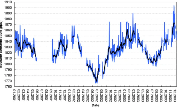
The instrument has been working for periods from 1997–2004, with a long break when the new station at Mt. Zeppelin was being built between June 1999 and March 2000. Other gaps in the record are due to system malfunctions. The data series is shown in Fig. 1. Despite the gaps in the data set, the seasonal variation is clearly 15

seen. Low methane concentration in summer and high in winter. The data series are too short to calculate a trend. Even so the data can be used in our analysis here to look at the frequency of high methane concentration episodes in Ny- ˚Alesund. These episodes typically last for 2 days and deviate more than 12 ppb (standard deviation) from the 14 days running mean of the data series.

20

3 Trajectory model and cluster analysis

The three-dimensional model of McGrath (1989) is used to calculate 5-day back-trajectories for the 4-year period 2000–2003. The choice of the duration of the tra-jectories is a compromise between the ambition to identify distant source- and sink-regions and the desire to limit uncertainties (Kahl et al., 1989; Stohl, 1998). In the 25

model, wind fields from the European Centre for Medium range Weather Forecasts (ECMWF) are used with a horizontal resolution of 1◦×1◦and temporal resolution of 6 h.

(6)

ACPD

Full Screen / Esc

EGU

Trajectories arriving at Ny- ˚Alesund are calculated twice a day (00:00 and 12:00 UTC) for the pressure level 850 hPa (Eneroth et al., 2003). The total number of trajectories for the whole period is 2860. They are classified into transport patterns through the use of cluster analysis. Cluster analysis is a variety of multivariate statistical analysis techniques designed to explore structure within a dataset and divide the dataset into 5

groups or “clusters” of similar cases. The idea is to maximize the similarity of indi-vidual group members while keeping separate groups as distinct as possible. In this study, the Ward minimum variance technique (Romesburg, 1984) is used to find the best clustering result. The cluster procedure is applied to all trajectories arriving at pressure level 850 hPa over Mt. Zeppelin station in Ny- ˚Alesund for the whole 4-year to 10

investigate year-to-year and month-to-month variability.

The combining of trajectories in clusters continues until all trajectories have been merged into one cluster. To decide where to stop the clustering, the total within-cluster spatial variance (TSV) was used (Moody and Galloway, 1988; Stunder, 1996) as a support. To few clusters would make it difficult to do a description of all the areas the 15

transport comes from and to many clusters would make it hard to distinguish between the clusters, thus the final choice1fell on 8 clusters for this analysis. The 8 clusters are shown in Fig. 2 and represent the eight different areas that the trajectories arriving at Ny- ˚Alesund came from 5 days earlier including their travel path. The use of clusters is a modification of classical wind-sector analysis. In addition to showing what sector the 20

air comes from it also accounts for the meteorology during days prior to arrival since the trajectories are shaped by variations in wind-speed and direction and clustered based on similarity in shape throughout the length of the trajectory.

1

(7)

ACPD

Full Screen / Esc

EGU

4 Results

4.1 Variability in trajectories

The atmospheric circulation and its seasonal variation affect the trajectory length and the clustering so that the longest trajectories occur during winter (strong cyclonic ac-tivity) and shortest during summer (weak mean pressure gradients). Typical clusters 5

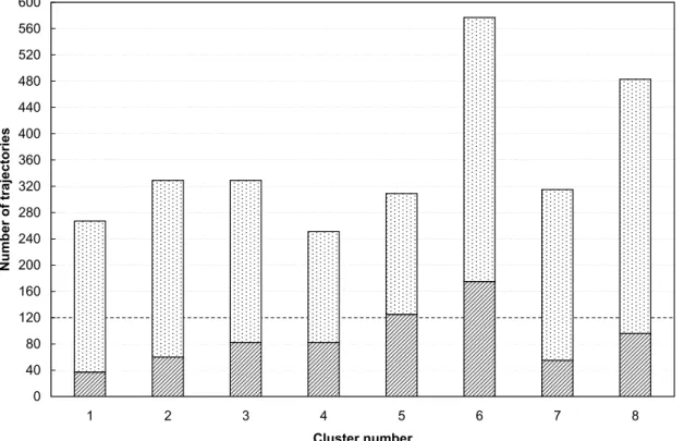
with summer situation are clusters 1, 2, 3, 5 and 7 (Fig. 2). A typical summer situation can be seen in cluster 2 where the trajectories are mainly within the Arctic Basin. In wintertime the situation changes and extensive cyclonic activity and stronger winds are more common. This gives longer trajectories and typical clusters for the winter Arctic are clusters 4, 6 and 8. Fig. 3 shows the distribution of total trajectories in each cluster 10

together with the fraction that has been below 950 hPa. 20% of the total clusters are found in cluster 6, thus this is the most common flow pattern on Mt. Zeppelin. Only 8% of the trajectories are found in cluster 4 thus this pattern is the least frequent at Mt. Zeppelin.

To see how the transport to Mt. Zeppelin station through the year the clusters are 15

divided into months and Table 1 shows how many trajectories there are in each cluster in each month.

Cluster 1 contains trajectories from North Canada, Alaska and some from Green-land. Most of the trajectories in this cluster are found in June (19%) and fewest in February (3%). This is defined as a summer cluster since this transport pattern is most 20

common in the summer months thus the methane concentration in this area during summer has opportunity to reach Mt. Zeppelin station.

Cluster 2 contains trajectories mainly from within the Artic Ocean. Most of the tra-jectories in this cluster are found in May (12%) and fewest in January (5%). This is a typical Arctic summer cluster with short trajectories (weak wind) origin from within the 25

Arctic basin. In this area there are few local sources of methane, thus when this cluster is dominant, there should be low methane concentrations at the station.

(8)

ACPD

Full Screen / Esc

EGU

trajectories in this cluster are found in July (14%) and fewest in January and March (4%). This is also defined as a summer cluster, though also in autumn there are many trajectories in this cluster. The length of the trajectories indicates weak winds and many of the trajectories are over ocean with few methane sources.

Cluster 4 contains trajectories from the Atlantic Ocean and North Canada. Most 5

of the trajectories in this cluster are found in December (14%) and fewest in March (3%). This is defined as a winter cluster. The trajectories have longer pathway indi-cating stronger winds and they come from areas with different methane sources like for instance wetlands and cities. Thus depending on time of year, the concentration reaching the station could vary.

10

Cluster 5 contains trajectories from the Atlantic Ocean and North Europe. Most of the trajectories in this cluster are found in July and October (14%) and fewest in March and December (3%). This cluster is not so easy to define, but since most of the trajectories are found in summer and autumn, it is a summer cluster. The trajectories arrive on the station mainly from south and the origin area have many methane sources, both 15

anthropogenic and natural.

Cluster 6 contains trajectories from North Europe and Russia. Most of the trajec-tories in this cluster are found in February and November (12%) and fewest in June (3%). This is a typical winter cluster with a lot of cyclonic activities in the Arctic and in addition this cluster is the one with most trajectories throughout the whole year (see 20

Fig. 3). Thus methane sources in this area should be seen more frequently in winter than in summer at the station.

Cluster 7 contains trajectories from Alaska and East Siberian. Most of the trajectories in this cluster are found in June (17%) and fewest in February (4%). This is again a summer cluster, but the trajectories origin is from the cost across the Artic basin. The 25

methane sources here should be mostly natural and most likely seen in summer. Cluster 8 contains trajectories from Central Siberian and Russia. Most of the trajecto-ries in this cluster are found in January (17%) and fewest in July (2%). This is a cluster were the trajectories have the cyclonic path witch is typical for the Arctic winter and is

(9)

ACPD

Full Screen / Esc

EGU

perhaps the most evident winter cluster. This cluster is the most interesting because the long-range transport of polluted constituents to the Arctic is most pronounced in winter and also because most the trajectory path is over strong source areas.

In Table 2 the number of trajectories is split into the different years they are occurring. The distribution of trajectories between the clusters shows little year-to-year variability. 5

Only in cluster 6 there is a clear decrease in percentage from 2000 to 2003. In the climatology from Eneroth et al. (2003) the total percentage from 1992–2001 in cluster 8 (comparable with cluster 6 in this work) is only 13% while here it is 20%. This means that there has been an increase in number of trajectories coming from the area North Europe and Russia. In addition the trajectories coming from Siberia represented in 10

Eneroth et al. (2003) as cluster 3 (comparable with cluster 8 in this work) has increased from 15% to 17%. This is a small increase, but totally it seems like the number of trajectories with origin in these areas have increased in the last years. In contrast the trajectories arriving from Alaska and Greenland (cluster 1 in both climatology) has decreased from 17% in Eneroth et al. (2003) to 9% in this work. This could indicate a 15

shift in the atmospheric flow patterns from over sea to over land. If there were more trajectories that travel over land before arriving at the Mt. Zeppelin station, this would have an impact on the frequency of methane episodes here.

4.2 Vertical motion

The vertical trajectory path also has to be considered in the clustering procedure. En-20

eroth et al. (2003) showed that the vertical transport of the trajectories is important since the air coming from aloft is different from the air that has been in contact with or near ground level. In the present clusters the trajectories path vary in vertical from 400 hPa to 1000 hPa height. If the air parcel has been in the boundary layer (below ap-proximately 950 hPa) it will be exposed to efficient mixing with surrounding air or altered 25

with direct contact to the surface and active sources there. The number of trajectories that has been below 950 hPa in the different clusters is seen in Fig. 3. In clusters no 1, 2, 7 and 8 less than 20% of the trajectories are under 950 hPa during the 5 days,

(10)

ACPD

Full Screen / Esc

EGU

whereas in cluster 5 more than 40% of the trajectories are in contact with ground. According to Stohl (2006) the air pollution can be transported into the Arctic along three different pathways: low-level transport followed by ascent in the Arctic, low-level transport alone, and uplift outside the Arctic, followed by descent in the Arctic. Only this last pathway is frequent for pollution originating from North America and Asia, whereas 5

European pollution can follow all three pathways in winter, and pathways one and three in summer.

In Fig. 3 cluster 5 (from Europe) has the highest percent of trajectories that has been below 950 hPa ones or several times and cluster 1 from Alaska/Greenland has lowest percentage. To see even better the seasonal variation Table 3 shows the percentage 10

divided into the different months. In consistent with Stohl (2006), cluster 5 has high percentage both in winter and summer, while cluster 1 has low percentage over the whole year. Notice that in December, there are no trajectories in cluster 1 that has been below 950 hPa during the 5 days. The same is true for cluster 7 (also partly from Alaska) in February. The time the trajectories have been below 950 hPa vary between 15

25 and 42 h for one 5-day trajectory. 4.3 Variability in methane

As an example of how the methane data from Mt. Zeppelin station can be used to-gether with the cluster analysis from previous section, hourly mean methane data for July 2002 is plotted directly with the different clusters in Fig. 4. Two of the winter clus-20

ters are marked especially, cluster 6 (red) and cluster 8 (brown). On 22 and 23 July, there is an episode with enhanced methane concentration and the trajectories arriv-ing at the station has been in cluster 8. On 27 and 28 July another episode is seen, the trajectories are now within cluster 6. These two clusters are transport from areas with strong methane sources like the Siberian wetlands, gas-fields and anthropogenic 25

sources in the cities. For these two times it is plausible that the air was transported form a polluted area to Mt. Zeppelin station with high methane concentration.

(11)

ACPD

Full Screen / Esc

EGU

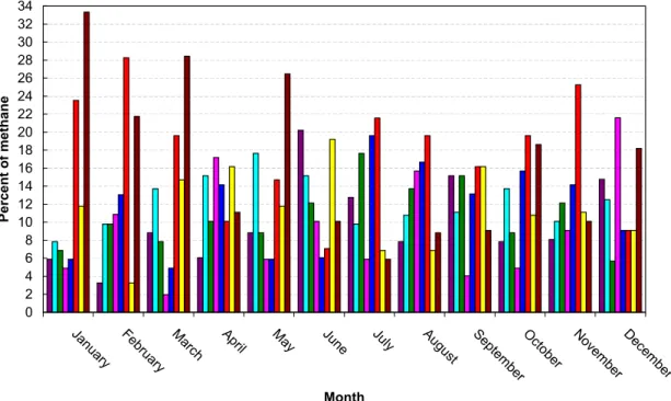
Mt. Zeppelin station, the amount of data in each cluster in each month must be con-sidered. Especially since the data series are not continuous. Although there are di ffer-ences between the distributions in Fig. 5 and Table 1, they are on the whole consistent because instrument failures have been evenly distributed around the year. The num-bers of data in each cluster are, however, important to consider in the next section 5

procuring differences in concentration in each cluster by season.

In Fig. 6 the mean of all the data (for all the years) with standard deviation is shown for each cluster throughout the year. The seasonal variation is clearly seen in all clusters, but there are some small differences between the clusters.

In cluster 1 the anthropogenic sources of methane are small, but wide expanses 10

with wetlands can be a large source of methane in spring when the thawing begins. This could be the reason for the mean in April to be higher than in March and May. The standard deviation is also small indicating stable high concentration with little variations in April, but only 6% of the methane samples are in this month. This cluster had most sampled methane data in June, but in summer the OH sink of methane is strongest 15

leading to low mean concentrations. In August is the standard deviation is low, hence there is little variation in the methane concentration. Though in December the standard deviation is high to be a summer cluster. The vertical motion of the trajectories could be the explanation of this since they have not been below 950 hPa, thus would preserve more of their original methane mixing ratio. If the sources in the area were varying this 20

would give a large standard deviation even if the mean methane in this month were close to the yearly mean.

Cluster 2 is representing mostly transport within the Arctic basin, and there are few sources of methane here. August is also a month with little variation in this cluster. Most of the summer has lower mean methane concentration than the yearly mean. 25

Cluster 3 contains trajectories arriving from the Atlantic Ocean and Greenland and has most of its data in July. Again August is the month with lowest standard deviation. In March the mean and standard deviation is large. This could be connected with the high percentage of the trajectories that has been below 950 hPa (43%). This could

(12)

ACPD

Full Screen / Esc

EGU

have change the methane mixing ratio in the air parcel and a possible source on the ground could give the high mean in this month.

In cluster 4 the transport is from the same area, but the trajectories are longer, reach-ing North Canada and further south in the Atlantic Ocean. Durreach-ing the summer the number of trajectories and data are high in this cluster and most of the trajectories 5

have their origin over land areas. The mean methane concentration is larger than the yearly mean most of the year, except in October. In this month it is the cluster with most trajectories that has been below 950 hPa (47%) and since the trajectories passes over large sea areas, it could be that the methane mixing ratio in the air parcel has decreased in contact with the marine boundary layer. In March 6 out of 8 trajectories 10

has been below 950 hPa, but this is not significant for the methane mean.

In cluster 5 from North Europe and the Atlantic Ocean, the seasonal variation is not so pronounced as in the previous clusters. This is an area with larger anthropogenic methane sources throughout the year, hence even during summer the OH-sink has not as strong effect and there is a high mean concentration in June. There are high stan-15

dard deviations throughout most of the year due to the high variation in the methane sources. It is a summer cluster (most trajectories in summer) and the cluster with high-est percent totally of trajectories below 950 hPa (41%). Due to all the strong anthro-pogenic methane sources along its pathways, there is a large variation and standard deviations in the data.

20

Cluster 6 is the cluster with most data in it (18% of total) and it is a winter cluster where February is the month with most data. June and August are months with small variations, but February, November and December have large standard deviation and the variation is most likely due to episodes of enhanced methane from the sources within this cluster. The low mean concentration in November could be explained similar 25

to the one in October in cluster 4. The trajectories are mostly from North Europe and Russia with large anthropogenic and natural methane sources leading to large variations in the data.

(13)

ACPD

Full Screen / Esc

EGU

September with little variations.

Finally in cluster 8 the trajectories comes from Central Siberia and Russia and this cluster contains 17% of the total methane data. These areas have strong emis-sions from the wetlands in summer (Christensen et al., 1995), but also anthropogenic sources from pipelines and cities. Most of the region is also covered with snow and ice 5

in winter, which means small sources of methane along the trajectory path. In January the transport to Ny- ˚Alesund is in the sectors defined by cluster 6 and 8 and the data are in these two clusters represent 35% of all the data. Also in February most trajectories are in clusters 6 and 8.

In summer time the weather conditions often produce light and variable winds in the 10

Polar Regions resulting in fewer trajectories in cluster 8 and from June to September the months have less than 6% of the trajectories. In August the mean is higher than the yearly mean, but the standard variation is low meaning small variations in the data. October, November and December has high variations in data for the same reason as in cluster 6. In these months the long-range transport of methane is efficient and the 15

OH-sink is absent. This causes frequent episodes of elevated methane at Mt. Zeppelin station, which is also seen in the data series (Fig. 1). The trajectories has seldom been below 950 hPa and thus preserved its mixing ratio good, though February is the month where most trajectories in this cluster has been in contact with the boundary layer, and this could be an explanation for the low mean in this month.

20

5 Discussion and conclusion

In this study the atmospheric flow patterns to Ny- ˚Alesund and their effect on the mea-sured methane concentration has been studied utilizing cluster analysis of trajectories for the 4-year period 2000–2003. Our trajectory pathways for the years 2000–2003 were compared to the climatology from Eneroth et al. (2003) for the period 1992–2001 25

and many similarities were found both in transport pattern in summer and winter. The trajectories were divided into 8 clusters that differ some from the first climatology

(14)

pe-ACPD

Full Screen / Esc

EGU

riod, but still comparable. There is a shift in three of the clusters with a decrease in the frequency of cluster 1 and 3 (from Alaska/Greenland) and an increase in the fre-quency of cluster 8 (from Central Siberian/Russia). This longer-term shift could have an effect on the measurements at Mt. Zeppelin station, both in methane and in other species since the winds thus are bringing in air with different “average” origin. Such 5

shifts in circulation can be due to natural climate variations (NAO/AO) or to even longer term climatic shifts or to human induced climate change. The wind shift with increased frequency of air passing over Siberia with origin in Europe are likely to give enhanced methane concentration both from the natural wetlands and from the anthropogenic sources like cities and gas fields (Tohjima et al., 1996). This could be misinterpreted 10

since it could yield an increase in background methane that is not necessarily related to changes in source or sink strengths, but rather frequency of transport from a par-ticular source area. This weakness in the present one-station analysis can only be remedied by combining data with a regional network of stations. Such a network is also necessary to determine neutral flux estimates of methane and is currently being 15

explored.

Another limitation to our study is the overlap in time of the to climatology studies. Ideally the trajectories for the whole period 1992–2003 should have been run again and clustered together. In this way, and with enough statistics, it will be possible to provide a comparison with the NAO/AO index to look for more climate shifts.

20

In summer, short trajectories often have their origin in air coming from areas in the Arctic and areas with small sources of methane. In contrast winter trajectories are fre-quently longer bringing air from sources farther away from Ny- ˚Alesund. These trans-ports can sometimes be seen as enhanced methane concentrations at the station. Peaks in the measurements with durations of up to several days are reoccurring fea-25

tures in the record. Notably in air arriving from central Siberia and Russia, there are high concentrations in springtime when the thawing of the tundra begins and probably releases methane. This observation merits further work in future studies and then in combination with remote sensing data where surface characteristics (thawing) can be

(15)

ACPD

Full Screen / Esc

EGU

quantified.

Svalbard is an island and there are few sources of methane in the area. Most of the methane variations above background2 values have been transported from sources afar. We conclude that methane has consistent behaviour with the other tracers with most influences from sources coming from Europe and Russia. We also showed that 5

the vertical motion of the trajectories is important for the methane concentration ob-tained at the Mt. Zeppelin station. If the trajectory has been below 950 hPa, the mixing ratio of methane in the air parcel will be affected by the methane concentration in the boundary layer.

Caution must be taken when interpreting concentration records and attempting to 10

derive source and sink distributions. Such shifts are even severer complications when proceeding further into attempting to determine and quantify possible shifts in the source and sink strengths. This also exposes a serious difficulty with attempting to de-termine regional flux rate responses to regional climate change since these transport shifts are in all likelihood caused by the same regional shifts in temperature patterns 15

that one may be attempting to correlate with rates of change in methane concentration at a station. An observational system that could enable the quantification of a regional climatologically response of a methane source must include a number of stations sur-rounding the region of interest, some interior stations, some local flux measurements, remote sensing data to enable continuous evaluation of the representativity (which will 20

vary through the seasons) of the local measurements and atmospheric models of ad-equate resolution to interpolate between the observational sites. The number of mea-surement stations of the different types described above can probably be gleaned from model studies of model variability assuming that our knowledge of meteorology (and thus wind calculations in transport models) incomplete as it may be, nevertheless, is 25

more robust than our grasp of methane fluxes and in particular these fluxes response to climate change. When designing an observational system and the observational network one will need periods of “oversampling” in space and time to verify that the

2

(16)

ACPD

Full Screen / Esc

EGU

number of stations is adequate and representative of the region one seeks to quantify fluxes for.

This could mean that the need for observation points in an observing system that allows continued quantitative monitoring of suspected regional source areas requires a substantially finer mesh than the presently available international greenhouse gas 5

observational network.

Acknowledgements. We are grateful to the Norwegian Pollution Control Authority (SFT) for

supporting the measurements at Mt. Zeppelin Station. This work has been supported by the Research Council of Norway (NFR; project no 142744/720) and EC project FP5 Contract EVK2-CT-2002-00175 Meth-MonitEUr.

10

References

Christensen, T. R., Jonasson, S., Callaghan, T. V., and Havstr ¨om, M.: Spatial variation in high-latitude methane flux along a transect across Siberian and European tundra environments, J. Geophys. Res., 100(D10), 21 035–21 045, 1995.

Dargaville, R. J., Law, R. M., and Pribac, F.: Implications of interannual variability in atmospheric

15

circulation on modelled CO₂concentrations and source estimates, Global Biogeochem. Cy-cles, 14(3), 931–943, 2000.

Dlugokencky, E. J., Houweling, S., Bruhwiler, L., Masarie, K. A., Lang, P. M., Miller, J. B., and Tans, P. P.: Atmospheric methane levels off: Temporary pause or a new steady-state? Geophys. Res. Lett., 30(19), 1992, doi:10.1029/2003GL018126, 2003.

20

Eneroth, K., Kjellstr ¨om, E., and Holm ´en, K.: A trajectory climatology for Svalbard; Investigating how atmospheric flow patterns influence observed tracer concentrations, Phys. Chem. Earth, 28, 1191–1203, 2003.

Harris, J. M., Tans, P. P., Dlugokencky, E. J., Masarie, K. A., Lang, P. M., Whittlestone, S., and Steele, L. P.: Variation in Atmospheric Methane at Mauna Loa Observatory Related to

25

Long-Range Transport, J. Geophys. Res. Atmos., 97, 6003–6010, 1992.

Harris, J. M., Dlugokencky, E. J., Oltmans, S. J., Tans, P. P., Conway, T. J., Novelli, P. C., Thoning, K. W., and Kahl, J. D. W.: An interpretation of trace gas correlations during Barrow, Alaska, winter dark periods, 1986–1997, J. Geophys. Res., 105, 17 267–17 278, 2000.

(17)

ACPD

Full Screen / Esc

EGU

Kahl, J. D., Harris, J. M., and Herbert, G. A.: Intercomparison of three long-range trajectory models applied to Arctic haze, Tellus, 41B, 524–536, 1989.

McGrath, R.: Trajectory models and their use in the Irish Meteorological Service. Irish Meteo-rological Service, Glasnevin Hill, Dublin, International Memorandum No 112/89, p 12, 1989. Moody, J. L. and Galloway, J. M.: Quantifying the relationship between atmospheric transport

5

and the chemical composition of precipitation on Bermuda, Tellus, 40B, 463-479, 1988. Paatero, J., Hatakka, J., Holm ´en, K., Eneroth, K., and Viisanen, Y.: Lead-210 concentration in

the air at Mt. Zeppelin, Ny- ˚Alesund, Svalbard, Phys. Chem. Earth, 28, 1175–1180, 2003. Pedersen, I. T. and Holm ´en, K.: Atmospheric methane at Zeppelin Station, Ny- ˚Alesund:

Presentation and analysis of in situ measurements, J. Environ. Monit., 7, 488–492,

10

doi:10.1039/b416934d, 2005.

Romesburg, H. C.: Cluster analysis for Researchers, Lifetime Learning Publications, Belmont, California, 129–135, 1984.

Stohl, A.: Computation, accuracy and applications of trajectories-a review and bibliography. Atmos. Environ., 32, 947–966, 1998.

15

Characteristics of atmospheric transport into the Arctic troposphere, J. Geophys. Res., 111, D11306, doi:10.1029/2005JD006888, 2006.

Stunder, B. J. B.: An assessment of the quality of forecast trajectories, J. Appl. Meteorol., 35, 1319–1331, 1996.

Tohjima, Y., Maksyutov, S., Machida, T., and Inoue, G.: Airborne measurements of atmospheric

20

methane over oil fields in western Siberia, Geophys. Res. Lett., 23(13), 1621–1624, 1996. Warwick, N. J., Bekki, S., Law, K. S., Nisbet, E. G., and Phyle, J. A.: The impact of meteorology

on the interannual growth rate of atmospheric methane, Geophys. Res. Lett., 29(20), 1947, doi:10.1029/2002GL015282, 2002.

(18)

ACPD

Full Screen / Esc

EGU

Table 1. Percent of trajectories in each cluster in each month for the period 2000–2003. Total

numbers of trajectories are 2860.

Cluster no 1 2 3 4 5 6 7 8 January 5.2 5.5 4.3 7.6 5.8 10.2 8.3 16.6 February 3.4 6.7 5.5 8.0 7.8 12.5 3.8 10.1 March 8.6 9.1 4.3 3.2 3.9 9.2 11.1 15.1 April 5.6 9.1 8.5 11.2 8.7 5.5 12.1 8.7 May 8.6 12.5 7.9 4.8 6.8 7.5 8.3 11.6 June 19.1 10.3 9.7 5.6 4.2 3.5 17.5 4.3 July 10.1 10.3 14.0 6.0 13.6 9.9 5.1 2.3 August 9.0 7.9 12.2 11.6 11.3 9.0 5.1 5.4 September 11.6 8.8 13.4 6.8 10.7 6.2 9.8 3.9 October 6.0 6.7 6.7 12.0 13.6 9.5 7.9 7.5 November 5.2 6.7 9.1 9.6 9.7 12.5 6.3 5.8 December 7.5 6.4 4.6 13.9 3.9 4.5 4.8 8.7

(19)

ACPD

Full Screen / Esc

EGU

Table 2. Percentage of trajectories in each cluster during different years.

Cluster no 1 2 3 4 5 6 7 8 2000 8.5 10.4 10.4 8.7 9.2 26.8 9.2 16.9 2001 7.8 14.4 9.2 8.9 11.8 19.9 10.7 17.4 2002 11.2 10.5 13.3 8.2 12.3 17.5 10.8 16.0 2003 9.9 10.6 13.3 9.3 9.9 16.2 13.6 17.2 2000–2003 9.3 11.5 11.5 8.8 10.8 20.2 11.0 16.9

(20)

ACPD

Full Screen / Esc

EGU

Table 3. Percent of trajectories that has been below 950 hPa in each cluster for each month.

Cluster no 1 2 3 4 5 6 7 8 January 21.4 16.7 21.4 42.1 72.2 49.2 30.8 26.3 February 11.1 31.8 38.9 25.0 37.5 27.8 0.0 30.6 March 21.7 30.0 42.9 75.0 50.0 34.0 11.4 27.4 April 6.7 20.0 28.6 28.6 44.4 53.1 2.6 28.6 May 4.3 7.3 26.9 50.0 33.3 20.9 11.5 7.1 June 17.6 8.8 9.4 21.4 30.8 5.0 18.2 9.5 July 3.7 17.6 17.4 20.0 35.7 7.0 37.5 9.1 August 37.5 11.5 7.5 10.3 42.9 13.5 25.0 7.7 September 6.5 6.9 31.8 35.3 33.3 36.1 29.0 10.5 October 6.3 18.2 22.7 46.7 42.9 27.3 8.0 8.3 November 28.6 27.3 33.3 33.3 36.7 44.4 35.0 17.9 December 0.0 38.1 53.3 34.3 33.3 38.5 6.7 17.3

(21)

ACPD

Full Screen / Esc

Printer-friendly Version Interactive Discussion EGU 1760 1770 1780 1790 1800 1810 1820 1830 1840 1850 1860 1870 1880 1890 1900 1910 01.2001 02.2001 03.2001 04.2001 05.2001 06.2001 07.2001 08.2001 09.2001 10.2001 11.2001 12.2001 01.2002 02.2002 03.2002 04.2002 05.2002 06.2002 07.2002 08.2002 09.2002 10.2002 11.2002 12.2002 01.2003 02.2003 03.2003 04.2003 05.2003 06.2003 07.2003 08.2003 09.2003 10.2003 11.2003 12.2003 Date Methane concentration (ppb)

Fig. 1. Daily mean (blue) with running 14 days mean (black) of in situ methane data at Mt.

(22)

ACPD

Full Screen / Esc

EGU

Fig. 2. Clusters obtained from the cluster analysis. Cluster 1: Alaska/Greenland, cluster 2: The

Arctic Ocean, cluster 3: The Atlantic Ocean/Greenland, cluster 4: The Atlantic Ocean/North Canada, cluster 5: The Atlantic Ocean/North Europe, cluster 6: North Europe/Russia, cluster7: Alaska/East Siberian, cluster 8: Central Siberian/Russia. A white circle is drawn around

Ny-˚

(23)

ACPD

Full Screen / Esc

Printer-friendly Version Interactive Discussion EGU 0 40 80 120 160 200 240 280 320 360 400 440 480 520 560 600 1 2 3 4 5 6 7 8 Cluster number Number of trajectories

Fig. 3. Total number of trajectories in each cluster depending on height, dotted area above

(24)

ACPD

Full Screen / Esc

EGU

Fig. 4. Hourly mean methane data (black) in July 2002 with coloured bars from cluster analysis:

Cluster 1-purple, cluster 2-turquoise, cluster 3-green, cluster 4-pink, cluster 5-blue, cluster 6-red, cluster 7-yellow and cluster 8-brown.

(25)

ACPD

Full Screen / Esc

Printer-friendly Version Interactive Discussion EGU cluster_stat.xls 0 2 4 6 8 10 12 14 16 18 20 22 24 26 28 30 32 34 Januar y Febr uar y Mar ch Apr

il May June July Augus t

September Oc_tober November December

Month

Percent of methane

Fig. 5. Percent of sampled methane data in each cluster in each month from 2001–2003

at Mt. Zeppelin station. Cluster 1-purple, cluster 2-turquoise, cluster 3-green, cluster 4-pink, cluster 5-blue, cluster 6-red, cluster 7-yellow and cluster 8-brown. These numbers differ from table 1 due to lack of methane data.

(26)

ACPD

Full Screen / Esc

EGU

Fig. 6. Monthly mean of methane (in ppb) with standard deviation from 2001–2003 for each