HAL Id: hal-00296046
https://hal.archives-ouvertes.fr/hal-00296046
Submitted on 6 Oct 2006
HAL is a multi-disciplinary open access
archive for the deposit and dissemination of
sci-entific research documents, whether they are
pub-lished or not. The documents may come from
teaching and research institutions in France or
abroad, or from public or private research centers.
L’archive ouverte pluridisciplinaire HAL, est
destinée au dépôt et à la diffusion de documents
scientifiques de niveau recherche, publiés ou non,
émanant des établissements d’enseignement et de
recherche français ou étrangers, des laboratoires
publics ou privés.
assimilated winds
B. Bregman, E. Meijer, R. Scheele
To cite this version:
B. Bregman, E. Meijer, R. Scheele. Key aspects of stratospheric tracer modeling using assimilated
winds. Atmospheric Chemistry and Physics, European Geosciences Union, 2006, 6 (12), pp.4529-4543.
�hal-00296046�
www.atmos-chem-phys.net/6/4529/2006/ © Author(s) 2006. This work is licensed under a Creative Commons License.
Chemistry
and Physics
Key aspects of stratospheric tracer modeling using assimilated winds
B. Bregman, E. Meijer, and R. ScheeleRoyal Netherlands Meteorological Institute, P.O. Box 201, 3730 AE, De Bilt, The Netherlands Received: 3 February 2006 – Published in Atmos. Chem. Phys. Discuss.: 6 June 2006 Revised: 7 September 2006 – Accepted: 26 September 2006 – Published: 6 October 2006
Abstract. This study describes key aspects of global chemistry-transport models and their impact on stratospheric tracer transport. We concentrate on global models that use assimilated winds from numerical weather predictions, but the results also apply to tracer transport in general circulation models. We examined grid resolution, numerical diffusion, air parcel dispersion, the wind or mass flux update frequency, and time interpolation. The evaluation is performed with as-similated meteorology from the “operational analyses or op-erational data” (OD) from the European Centre for Medium-Range Weather Forecasts (ECMWF). We also show the ef-fect of the mass flux update frequency using the ECMWF 40-year re-analyses (ERA40).
We applied the three-dimensional chemistry-transport Tracer Model version 5 (TM5) and a trajectory model and performed several diagnoses focusing on different transport regimes. Covering different time and spatial scales, we ex-amined (1) polar vortex dynamics during the Arctic winter, (2) the large-scale stratospheric meridional circulation, and (3) air parcel dispersion in the tropical lower stratosphere.
Tracer distributions inside the Arctic polar vortex show considerably worse agreement with observations when the model grid resolution in the polar region is reduced to avoid numerical instability. The results are sensitive to the diffu-sivity of the advection. Nevertheless, the use of a computa-tional cheaper but diffusive advection scheme is feasible for tracer transport when the horizontal grid resolution is equal or smaller than 1 degree. The use of time interpolated winds improves the tracer distributions, particularly in the middle and upper stratosphere. Considerable improvement is found both in the large-scale tracer distribution and in the polar re-gions when the update frequency of the assimilated winds is increased from 6 to 3 h. It considerably reduces the vertical dispersion of air parcels in the tropical lower stratosphere. Correspondence to: B. Bregman
Strong horizontal dispersion is not necessarily an indica-tion of poor wind quality, as observaindica-tions indicate. More-over, the generally applied air parcel dispersion calculations should be interpreted with care, given the strong sensitivity of dispersion with altitude.
The results in this study provide a guideline for strato-spheric tracer modeling using assimilated winds. They fur-ther demonstrate significant progress in the use of assimilated meteorology in chemistry-transport models, relevant for both short- and long-term integrations.
1 Introduction
Global three-dimensional chemistry transport models (here-after referred to as CTMs) driven by actual meteorology from numerical weather predictions are crucial for the interpreta-tion of many observainterpreta-tional data. The great advantage is the direct comparison with observations by their ability to uti-lize actual meteorology to drive the model transport. CTMs are thus ideally designed for detailed sensitivity studies of key processes important for climate, which would be com-putationally too expensive for Chemistry-Climate Models (CCMs). Major areas of interest are the polar regions, ow-ing to the prevailow-ing chemical ozone loss durow-ing winter and their sensitivity towards climate change, and the tropical re-gion where the main entrance of air into the stratosphere is located (Holton et al., 1995).
The ability of a direct comparison with observations also allows model sensitivity studies to investigate basic model parameters, such as grid resolution and advection, but also the quality of the mass fluxes (or wind vectors) and the way the meteorological information is implemented in the CTM. The impact of grid resolution on the atmospheric compo-sition remains an important subject of discussion. Searle et al. (1998) show that a horizontal resolution of 3◦is suf-ficient to calculate polar chemical ozone loss. In contrast,
Marchand et al. (2003) found substantial differences after in-creasing their model resolution from 2◦×2◦to 1◦×1◦.
An-other model study also focused on the effect of spatial reso-lution in the polar region by evaluating methane distributions (van den Broek et al., 2003). An important outcome was the significant overestimation of methane in the lower strato-sphere at the edge and inside the polar vortex. An increase of the horizontal grid resolution to 1◦×1◦gave negligible im-provement and thus indicated very small sensitivity to hor-izontal resolution. A similar conclusion came from Searle et al. (1998) and Strahan and Polansky (2006). However, Searle et al. (1998) stated that the sensitivity to resolution de-pends on the diffusivity of the advection scheme. The results of this study underlines this conclusion, contrast our earlier findings by van den Broek et al. (2003) and are more in line with those from Marchand et al. (2003).
However, the investigation of grid resolution in the polar regions is complicated by the commonly applied grid cell or mass flux merging which is done to avoid numerical prob-lems. CTMs and CCMs suffer from numerical instability in regions of strong zonal winds and relatively small grid cells. The most critical regions are located at the poles, in particu-lar during the winter, but also in the vicinity of storm tracks. Negative tracer mass can occur when the transport distance during one advection time step exceeds the size of the grid cell, the so-called Courant-Friedrichs-Lewy (CFL) criterion. This is generally solved by reducing the grid resolution or by averaging the wind vectors or mass fluxes, but its impact on tracer transport has sofar not been investigated.
An obvious alternative solution would be to reduce the ad-vection time step, but this would lead to excessively small time steps. To overcome this difficulty we introduced an iter-ation procedure for tracer advection in the TM5 model with locally adjusted time steps (Krol et al., 2005). This iteration procedure allowed us to omit the model grid averaging (apart from the pole cap itself). In Krol et al. (2005) the focus was on the troposphere. In this study we will demonstrate the dramatic impact on the stratospheric tracer distribution.
Another crucial factor for tracer transport is the quality of the winds provided by the numerical weather predictions. The winds are subject to data assimilation within the model prediction and are often referred to as Data Assimilation Sys-tem or DAS winds (Schoeberl et al., 2002). The quality of particularly the stratospheric winds is affected by the pres-ence of spurious variability or “noise”, inherently introduced through the assimilation procedure, either through a lack of suitable observations or by inaccurate treatment of the model biases. This unwanted variability causes enhanced disper-sion or spurious mixing that accumulates in time (Stohl et al., 2004; Tan et al., 2004). Hence, the impact of dispersion in-creases with increasing dynamic time scales. It may there-fore not be a serious problem for the troposphere where the dynamic turnover times are relatively short. However, the stratospheric circulation contains much longer time scales where spurious variability in DAS winds becomes very
crit-ical. One of the consequences is enhanced dispersion and an enforced large-scale stratospheric meridional circulation, causing tracer residence times to be considerably shorter than observed (Schoeberl et al., 2002; Douglass et al., 2003; Mei-jer et al., 2004). The most critical region is the tropical lower stratosphere, where the majority of the air enters the strato-sphere. Moreover, this is a very complicated region for data assimilation due to a lack of observations and because the tropical atmosphere is not in geostrophical balance, which complicates proper treatment of model biases.
Meijer et al. (2004) and Scheele et al. (2005) show that the intensity of dispersion in the DAS winds increases when the assimilation procedure is less accurate or less sophisti-cated. For example, the ECMWF utilizes three- and four-dimensional assimilation procedures (3DVAR and 4DVAR respectively). 4DVAR is a temporal extension of 3DVAR, and thus more accurate but also computationally more ex-pensive. A comprehensive description of the ECWMF as-similation procedures can be found at http://www.ecmwf.int. A major difference is that 4DVAR produces physically more balanced winds for each model time step, due to the inclusion of time. Because of computational expenses the ECMWF 40-year re-analyses (ERA40) have been produced with 3DVAR, while the operational data, analyses and forecasts (referred to as “Operational Data” or OD) have been produced with 4DVAR. Comparing both data sets thus yields information about the impact of assimilation accuracy on tracer transport. Ozone is a useful tracer, since its distribution is very vul-nerable to the strength of large-scale stratospheric circula-tion. Laat et al. (2006) and Noije et al. (2004) show a very strong accumulation of ozone in the extra-tropical lower stratosphere when using ERA40 winds, resulting in signif-icant overestimation compared to observations. When ap-plying OD winds, the agreement becomes much better. In-deed, Noije et al. (2004), Simmons et al. (2005) and Scheele et al. (2005) have shown that OD winds contain less disper-sion than ERA40 winds in the tropical lower stratosphere and provide more realistic extra-tropical downward ozone fluxes (Noije et al., 2004) and more realistic stratospheric residence times (Meijer et al., 2004). However, even with OD the cir-culation remains too strong (Laat et al., 2006), which has led to the practical decision to constrain stratospheric ozone down to 100 hPa in the extra-tropics with ozone climatol-ogy (Noije et al., 2004) for the tropospheric multi-year IPCC chemistry-transport runs . However for coupled troposphere-stratosphere runs this solution is undesirable.
Recently, a comprehensive model intercomparison was performed with winds and temperatures from a variety of data assimilation systems, focusing on the 2002 Antarctic vortex split (Manney et al., 2005). They show substantial differences between the models that apply different DAS, with operational (4DVAR) analysis performing better than re-analysis (3DVAR) data, consistent with the studies de-scribed above.
Despite shortcomings in ERA40 winds, the dynamical variability can be simulated quite well (Hadjinicolaou and Pyle, 2005; Chipperfield, 2006). This is in line with a comparison between DAS winds from different numeri-cal weather predictions, where ERA40 winds were found to agree excellent with observed variability (Randel et al., 2003). Therefore the ERA40 data is regarded as one of the most valuable meteorological data sets for long-term trend studies. It is for this reason that we added ERA40 to our di-agnostics. The crucial question is if there are ways to use ERA40 data in CTMs that improve the stratospheric tracer transport.
One relevant aspect not commonly addressed in CTM studies is the effect of the update frequency of the assim-ilated winds and the variability within the time interval on the modeled tracer distributions. Generally the winds are up-dated every 6 h. However, stratospheric dynamical variabil-ity occurs on time scales shorter than 6 h (Shepherd et al., 2000; Manson et al., 2002), so that a considerable part of real variability is neglected. Additionally, the winds can be assumed constant over this time interval (instantaneous), av-eraged or interpolated in time. Instantaneous winds intro-duce discontinuities when changing time interval, leading to spurious variability (aliasing), while averaging can be re-garded as a (strong) wave filter. Examining ERA40 winds with the FLEXPART trajectory model (Stohl et al., 2002), Legras et al. (2005) show that decreasing the meteorological update time interval from 6 to 3 h reduces spurious motions in the stratosphere considerably.
There have only been very few model studies using 3-hourly meteorological data in CTMs (Wild et al., 2003; Legras et al., 2005; Berthet et al., 2006). Moreover, a more general evaluation at different spatial scales and including the effect of interpolation within the time interval has not yet been performed, which is the aim of this study.
The important question is whether we will be able to perform meaningful multi-year tracer integrations applying DAS winds. The answer depends on the progress in im-proving DAS wind quality and the way they are applied in global models. Improving the quality of DAS winds is an ongoing activity and progress is being made in filtering tech-niques, treatment of the error covariances and bias correc-tions (Polavarapu et al., 2005), Simmons, personal commu-nication). In this study we concentrate on how DAS winds are applied in CTMs.
To evaluate all these key aspects for tracer transport we perform a variety of integrations, examining different model grid resolutions, as well as different time intervals of the DAS winds, including time interpolation effects. We use CH4as
a passive tracer to focus on polar transport in a similar set-up as in van den Broek et al. (2003). The reason for this experiment is not to provide a detailed evaluation of transport in the Arctic polar vortex, but rather to supply an update of our previous model evaluation.
We further apply the age of air diagnose as a first-order approximation of the impact on the large-scale stratospheric meridional circulation and perform trajectory calculations to examine the degree of dispersion in the tropical lower strato-sphere in the assimilated winds. All CTM experiments have been performed with ECMWF operational analyses, while the ECMWF re-analyses, ERA40, has been used in trajectory experiments to illustrate the effect of meteorology update fre-quency. We have decided not to use ERA40 fields in our CTM studies since it is known that the stratospheric tracer distributions are of worse quality using re-analyses data in-stead of operational analyses.
The outline of this paper is as follows. We first briefly describe TM5 and the recent updates. The next section de-scribes the model sensitivity experiments for the polar re-gion, the general stratospheric circulation and dispersion in the tropical lower stratosphere, which is followed by a sec-tion describing the results for each diagnostic. Some aspects subject for discussion are addressed in the Discussion sec-tion, which is followed by the section Conclusions.
2 Model description
The CTM we use in this study is the global Tracer Model, TM5, which is a grid point Eulerian 3-D CTM and an ex-tended version of the TM3 model. The TM3 model has been used widely in the modeling community (e.g. Dentener et al., 1999; Peters et al., 2001; Houweling et al., 1998; Van den Broek et al., 2000; Bregman et al., 2001, 2002). The orig-inal version of the model has been developed by Heimann (1995); Heimann and Keeling (1989). TM5 uses forecasts of the European Centre for Medium-range Weather Forecasts (ECMWF) to drive the transport with a default update time interval of 6 h. It further uses mass fluxes for advection of the tracers as described in van den Broek et al. (2003). The model contains a Cartesian grid and consists of a two-way nested grid zooming over selected areas by increasing the horizontal resolution, currently up to 1◦×1◦. The model fur-ther contains hybrid σ -pressure levels with the top level at 0.1 hPa. The representation of the model winds has been ad-justed to assure mass conservation following the method of Segers et al. (2002), which improved the representation of the model tracer fields significantly (Bregman et al., 2003).
An important feature of the TM5 zoom version is the mass consistent two-way nesting that allows global studies includ-ing zoom areas. Because of the grid zoominclud-ing capability the model architecture has changed fundamentally. The model structure and the zooming concept have been described in detail and the model was successfully validated for the lower troposphere by Krol et al. (2005).
A validation of stratospheric tracers was performed by van den Broek et al. (2003). The TM5 version used in this study differs in important aspects from the version used by van den Broek et al. First, in their study the advection scheme
contained only first-order moments or slopes (Russel and Lerner, 1981). In this study also second-order moments ad-vection (Prather, 1986) is applied.
The second crucial difference is the introduction of ad-justable advection time steps when the CFL criterion is vi-olated. This update avoids grid cell averaging in the polar re-gions. In all our previous model studies mass flux or grid cell averaging, referred to as “polar grid reduction” (labeled as “red. grid” in Table 1) was necessary in the stratosphere since the model did not contain iterative advection. See Sect. 2.3 in Krol et al. (2005) for a detailed description of the reduced grid treatment in TM5. In van den Broek et al. (2003) the re-duced polar grid is illustrated within the zoom grid in Fig. 1 of that paper. Grid cell averaging was performed over the longitude for each polar latitude down to 70◦N. For numeri-cal stability the pole cap remains one grid cell.
The third difference involves the possibility to apply time interpolation between the meteorology update intervals and the use of 3-hourly meteorology.
The final difference involves the vertical resolution. In the previous model evaluation by van den Broek et al. (2003) 33 layers were applied from the original ECWMF 60-layer coor-dinate by reducing some layers in the upper stratosphere and lower troposphere. In this study we used 45 layers, including all stratospheric levels. We have performed sensitivity runs with passive CH4 and varied the number of vertical layers
between 30 and 60, but the differences in the lower strato-sphere were negligible (not shown). This is in line with the findings from Strahan and Polansky (2006) who found dif-ferences mainly in the upper stratosphere and mesosphere.
Without iterative advection the reduction of the polar grid cannot be validated because of computational limits, since the advection time steps would not only become excessively small (i.e. a few minutes only), but they would also have to be applied over the whole model domain. The new advection algorithm allows sufficiently small advection time steps by means of an iteration procedure for the location where a CFL violation occurs, rather than by applying it over the whole grid. Whenever a CFL violation occurs, the required number of iterations is determined by reducing the mass fluxes ac-cordingly until the violation is solved. Then the advection is performed with the required number of iterations.
At the location where the violation occurred, the iteration is performed differently, depending on the mass flux direc-tion. Zonally: for every longitude at the specific latitude. Meridionally: for every latitude and longitude at the specific pressure level. Vertically: for all model grid cells. In practice the majority of violations occur in the zonal direction where the winds are the strongest.
The iteration procedure has extensively been tested for nu-merical errors by using idealized passive tracers, and the er-rors remained close to machine precision (not shown). This model update was crucial, since it not only allows integra-tions at higher model grid resoluintegra-tions but also allows a proper examination of model grid resolution.
The default configuration of TM5 in this study includes a global horizontal resolution of 3◦×2◦ (longitude ×
lati-tude), 45 vertical layers and a second-order moment advec-tion scheme (Prather, 1986). It further applies instantaneous wind fields from the ECMWF operational analyses updated every 6 h.
In addition to the default model configuration we included a computationally cheap but diffusive first-order advection scheme (“slopes”) (Russel and Lerner, 1981) and applied a zoom grid with a horizontal resolution of 1◦×1◦ between 30◦–90◦N, similar as in van den Broek et al. (2003) (see their Fig. 1). Note that with the current model configuration, inte-grations including a zoom area could only be performed with the first-order advection scheme. This is because a second-order moments advection introduces additional communica-tion between the different zoom regions and requires funda-mental changes in the model transport modules which were not feasible to perform.
For the trajectory experiment the trajectory model is used as described by Scheele et al. (2005).
3 Experimental set-up
This study contains a variety of model experiments includ-ing the CTM and the trajectory model. A summary of the model experiments with the main features including the di-agnostics is given in Table 1. The model evaluation covers two important regions: the Arctic polar vortex and the tropi-cal stratosphere and three different diagnostics: passive CH4
tracer integrations, mean age of air calculations and air parcel dispersion. The experimental setup for the different diagnos-tics is given below.
3.1 Passive CH4
This CTM diagnostic covers the Arctic region and uses CH4
as a passive tracer. The model was integrated from Septem-ber 1999 to April 2000. The experimental setup, including the model constraints, is similar as in van den Broek et al. (2003), which we summarize below.
Initialization is based on zonally averaged observations of August and September 1999, obtained from the HALOE 10 (HALogen Occultation Experiment) instrument aboard UARS (Upper Atmospheric Research Satellite) (Russel-III et al., 1993). In regions for which observations are not avail-able (at the poles, in the troposphere and in a gap in the HALOE data between 43◦N and 62◦N), the initial
concen-trations are linearly inter- or extrapolated from nearby lati-tudes and/or altilati-tudes.
The CH4, concentrations in the lowest model layer are
fixed at 1.76 ppmv. In the top two levels CH4is constrained
with HALOE observations (Randel et al., 1998), since chem-ical destruction of CH4 is not included in the model.
Table 1. A summary of the model experiments. See text for more details for each experiment.
Experiment advection horizontal resolution winds diagnose “6hrly inst.” 2nd moments 3◦×2◦ 6-hourly instantaneous “OD” CH4, Mean age of air
“6hrly inst. red. grid” 2nd moments 3◦×2◦ 6-hourly instantaneous “OD” CH4
“3×2-slopes red. grid” 1st moments 3◦×2◦ 6-hourly instantaneous “OD” CH4, Mean age of air
“3×2-slopes” 1st moments 3◦×2◦ 6-hourly instantaneous “OD” Mean age of air “1×1-slopes” 1st moments 1◦×1◦ 6-hourly instantaneous “OD” CH4, Mean age of air
“6hrly interp.” 2nd moments 3◦×2◦ 6-hourly interpolated “OD” CH4, Mean age of air, Dispersion “3hrly interp.” 2nd moments 3◦×2◦ 3-hourly interpolated “OD” CH4, Mean age of air, Dispersion
“6hrly interp. ERA40” 2nd moments 3◦×2◦ 6-hourly interpolated “ERA40” Dispersion “3hrly interp. ERA40” 2nd moments 3◦×2◦ 3-hourly interpolated “ERA40” Dispersion
that prescribing the top boundary concentrations have only a small or negligible effect on the tracer fields for the consid-ered integration period. In addition, they found that ignoring chemical destruction of CH4causes a small deviation of less
than 10%, and only above 10 hPa.
The observations were obtained from the balloon-borne Tunable Diode Laser Absorption Spectrometer (TDLAS) (Garcelon et al., 2002), the Jet Propulsion Laboratory MkIV interferometer (Toon et al., 1999), and the space-borne HAlogen Occultation Experiment (HALOE) (Russel-III et al., 1993) on board the UARS satellite. The balloon-borne observations were performed in the frame of the com-bined projects THird European Stratospheric Experiment on Ozone (THESEO) and Sage III Ozone Loss and Validation Experiment (SOLVE).
This diagnostic focuses on the high latitudes, since methane is treated as a passive tracer. For this reason the in-tegration period is not more than half a year, but is sufficient for the purpose of this experiment. However, caution must be taken for mid-latitudes in the middle and upper stratosphere where the impact of chemistry becomes more pronounced.
3.2 Mean age of air
The mean age of air is calculated by applying the “tracer pulse” method, as described in Hall and Plumb (1994) and Hall et al. (1999). The tracer pulse method consists of an in-ert tracer released in the tropical troposphere with unity mass mixing ratio by applying a delta-function. The tracer is re-leased in a latitude band between 10◦S and 10◦N and up to
200 hPa during the first model step and set to zero afterwards (Meijer et al., 2004). The released tracer is transported to the stratosphere and the tracer mixing ratios in the stratosphere are a measure of the mean residence time, calculated using the Green function (Hall and Plumb, 1994). The year 2000 is integrated repetitively for 20 years. The mean age is cal-culated as the first moment of the derived spectrum after 20 years.
3.3 Air parcel dispersion
Using the same experimental setup as in Scheele et al. (2005) we examined the dispersion of air parcels in the tropical lower stratosphere by calculating 50-day back trajectories similar to the experiments performed by Schoeberl et al. (2002). We used January and February 2000 meteorology. Approximately 10 000 trajectories started between 10◦S–
10◦N at 460 K potential temperature level, corresponding to
a pressure of 50 hPa or approximately 20 km altitude. As a measure of dispersion, the fraction of air parcels is calcu-lated crossing the tropopause irriversibly. The tropopause is defined on basis of potential vorticity and close to the equa-tor as the 380 K potential temperature level (Scheele et al., 2005). In this diagnose we have applied ECWMF 6-hourly interpolated operational analyses and 6-hourly and 3-hourly interpolated ERA40 re-analyses (see Table 1).
4 Results
4.1 Passive CH4
4.1.1 Comparison with balloon-borne profiles inside the polar vortex
We show a series of figures with comparisons of calculated by the CTM and observed CH4 profiles. The observations
consist of single balloon- and space-borne profiles sampled in the polar vortex from December 1999 to April 2000 from Kiruna (67.8◦N, 20.4◦E). The selected balloon profiles were all inside the polar vortex and represent the evolution of the tracer profiles during the winter. The reason for this se-lection is because in one of our previous model evaluation (van den Broek et al., 2003) the largest model overestimation was found for these profiles.
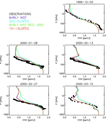
Figure 1 shows a comparison with observations for the CTM experiments “6hrly inst”, “6hrly inst red. grid”, “3×2-slopes red. grid”, and “1×1-“3×2-slopes” (see Table 1 for an overview of the model experiments). The model profiles
Fig. 1. Instantaneous methane profiles (ppmv) versus pressure (hPa), observed (black dots), and calculated by the model (solid lines) at 15 March 2000. The horizontal bars denote the 2-σ obser-vational uncertainty. The color lines represent the calculated pro-files from the different model experiments.
were calculated for the location of the balloon launch with bi-linear interpolation using the adjacent grid cells. Differ-ent interpolation methods did not change the profiles (not shown). The observed decrease with altitude of CH4
pro-files in Fig. 1 become stronger during the winter, reflecting the descent of the polar vortex air. In December the model results are close to the observations. However, the model overestimates CH4later in the winter and the overestimation
increases in time. For clarity we have added the “3×2-slopes red. grid” results from van den Broek et al. (2003) which considerably overestimate the observed CH4profiles. When
applying the less diffusive second-order moments advection the overestimation reduces significantly and clearly shows the large sensitivity of tracer transport towards diffusive ad-vection. This is even better illustrated when examining the results from the “1×1-slopes” experiment. The diffusivity of the first-order advection reduces considerably when increas-ing the horizontal resolution to 1◦×1◦. Now the results are very similar to the profiles calculated by the “6hrly inst.” ex-periment.
Nevertheless the model still overestimates the tracer con-centrations. The results from the “6hrly inst red. grid” exper-iment reflects the effect of the reduced polar grid. Although this experiment is performed with the less diffusive second-order moments advection, the calculated profiles are
signif-Fig. 2. As signif-Fig. 1, but with the results from the model experiments
applying interpolated winds and increased meteorology update fre-quency.
icantly overestimated and the discrepancy increases in time. This quite dramatic effect clearly shows the large sensitivity towards horizontal resolution.
The improvement when removing the reduced polar grid gives an important message to those who apply some kind of grid or mass flux or wind vector merging in the polar re-gion. Another obvious message is that a reduction of the polar grid obscures evaluation of grid resolution. In van den Broek et al. (2003) their “1×1-slopes” experiment did not improve the calculated CH4profiles because that model
ver-sion still contained the same polar grid averaging as in the coarser resolution setup.
Finally, we examined the effect of time interpolation and wind update frequency. Figure 2 shows the calculated CH4
profiles from the experiments “6hrly inst”, “6hrly interp” and “3hrly interp”. By interpolating the winds between two sub-sequent time intervals we account for the wind variability within the model integration time interval. The agreement with observations improves, especially on 15 March 2000. Applying 3-hourly interpolated winds the results are in ex-cellent agreement with the observations.
4.1.2 Horizontal cross sections in the polar region
Figures 1 and 2 show that the model errors accumulate in time during the winter. Subsequently, the profile at the end of the winter on 15 March 2000 is quite interesting, since for
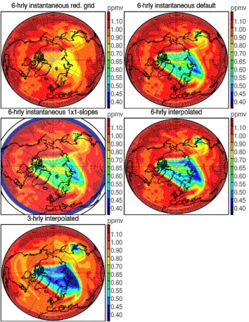
Fig. 3. Horizontal cross sections of methane mixing ratios (ppmv)
at 35 hPa, 15 March 2000, 00:00 GMT for five different TM5 ex-periments.
this day the model discrepancies are most visible and the vor-tex was still very strongly developed, as was demonstrated in previous model intercomparison (van den Broek et al., 2003). Therefore we focus on this day and examined the polar vor-tex with horizontal cross sections of CH4at 35 hPa.
Figure 3 shows the results for the “6hrly inst.”, “6hrly inst. red grid”, and “1×1-slopes” experiments all using hourly instantaneous winds, and for the experiments with 6-hourly and 3-6-hourly interpolated winds. The CH4levels from
the reduced grid run are clearly higher with a very weak vor-tex edge and little tracer variability compared to the fields from the other experiments. The “6hrly inst.” and the “1×1-slopes” runs yield much stronger vortex edges and more vari-ability and both fields are quite comparable. The vortex edge tracer gradients will be shown in more detail in Figs. 5, 6 and 7. The vortex gradients become slightly stronger when using 6-hourly interpolated winds, but significantly stronger when using 3-hourly interpolated winds. Note that also out-side the vortex the tracer fields are conout-siderably lower in this model version, indicating that applying time interpola-tion and in particular increasing the update frequency affect the tracer distribution on a large (hemispheric) scale. Berthet et al. (2006) also shows reduction in N2O, HNO3and NO2in
m rxm, rym, rzm rxxm, rxym, rxzm ryym, ryzm, rzzm m rxm, rym, rzm m rxm rym rzm m rxm rym rzm m rxm rym rzm m rxm rym rzm m rxm rym rzm m rxm rym rzm 'default' 30x20 'slopes' 30x20 'slopes' 10x10
Fig. 4. A schematic view of the tracer information per grid cell of
3◦×2◦, when applying second-moments (left) and first-order advec-tion without grid zooming (middle) and with grid zooming (right).
the mid-latitude middle stratosphere when applying 3-hourly winds compared to 6-hourly winds.
4.1.3 Diffusivity and model grid resolution
The strong sensitivity of tracer advection to diffusivity is in-teresting, as shown by the results from the “1×1-slopes” ex-periment. Numerical diffusion depends on the amount of tracer information for a given grid cell volume. Figure 4 shows the tracer information for a 3◦×2◦ grid cell in the case of the default “6-hourly inst” experiment (left panel), the “3×2-slopes” experiment (middle panel) and the “1×1-slopes” experiment (right panel). The “6-hourly inst” ex-periment contains 10 parameters that determine the tracer level: the first-order slopes (3), the second-order moments (6), and the tracer mass (1). In contrast, the “3×2-slopes” experiment only contains 4 variables with tracer informa-tion: the first-order slopes (3) and the tracer mass (1). On the other hand, the zoom region (“1×1-slopes” experiment) contains 6 more grid cells with each 4 tracer parameters, re-sulting in a total of 24 on basis of a 3◦×2◦grid cell. The “3×2-slopes” experiment contains the least amount of tracer information and clearly yields the worst results. However, the amount of tracer information in the “1×1-slopes” exper-iment is twice more than that of the “6-hourly inst” config-uration for a 3◦×2◦grid cell, but shows no improvement in the tracer distribution. This insensitivity to grid resolution supports the findings by Searle et al. (1998) although it de-pends on the diffusivity of the tracer advection. A diffusive advection scheme clearly overrules the advantage of resolu-tion increase, at least up to 1◦×1◦. It will also depend on the
chemical lifetime of the tracer in question and for a relatively short-lived species such as ClO the impact of resolution in-crease may be substantial (Marchand et al., 2003; Tan et al., 1998).
4.1.4 Comparison with satellite observations: tracer gradi-ent across the vortex edge
Next, we focus on the tracer gradient through the vortex edge. A comparison is performed with 15 profiles observed by the HALOE instrument on board the UARS satellite. See van den Broek et al. (2003) for a more detailed description of these observations. These profiles were part of the HALOE
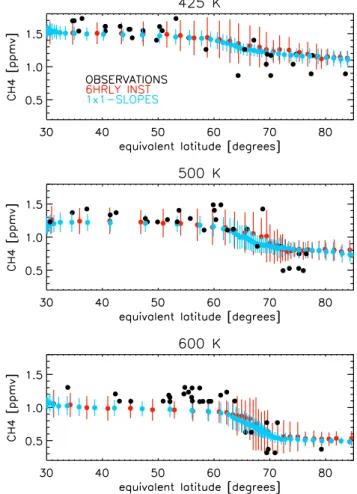
Fig. 5. Observed methane profiles volume mixing ratios in ppmv
(black dots) at 15 March 2000, 00:00 GMT, and calculated by the model using 6-hourly instantaneous winds, “6hrly inst”. (red dots) and the model run without the reduced polar grid, “6hrly inst. red. grid”. The comparison is performed at equivalent lati-tude (degrees) and three different isentropic levels (425 K, 500 K, and 600 K). The vertical bars represent 2σ variability of the model results.
sweeps close to the edge of the polar vortex, covering both mid-latitudinal extra- and polar vortex air, and are thus very suitable to focus on the vortex edge. For such a comparison an equivalent, instead of the regular Cartesian, latitude coor-dinate is more useful. Three different potential temperature levels have been selected, one close to the polar vortex bot-tom (425 K), one in the lower stratosphere (500 K) and one in the middle stratosphere (600 K).
Figures 5, 6 and 7 show the results of this comparison for different CTM experiments. Each equivalent latitude contains several model values and each point represents the mean model value and the vertical bars represent the variabil-ity as 1σ . Each of these figures contains the results from the “6hrly inst” experiment compared with the results from an-other experiment. The reason is to allow a clear comparison of the different model versions with the default model
ver-Fig. 6. Similar as ver-Fig. 5, but with the results from the experiments
“6-hourly inst.” (red dots) and “1×1-slopes” (blue dots).
sion. For clarity we left out the “6hrly interp.” experiment, since the results are very similar to those from the “6hrly inst” experiment.
The comparisons are somewhat obscured by the relatively large scatter in the observations, the limited coverage in the polar vortex and the modeled variability. The scatter in the observations is most probably due to the differences in the sampling volume of the observations and the ECWMF po-tential temperature and popo-tential vorticity grid cell volumes. Nevertheless, the latitudinal coverage is sufficient and the tracer gradient and variability across the vortex edge are clearly discernible. As expected, the gradient becomes more pronounced with increasing potential temperature level, both in the observations and in the model results. The results from the “6hrly inst” experiment agrees quite reasonable with the observations, while significant underestimation is found when applying polar grid averaging (“6hrly inst red. grid”), in line with the findings in Fig. 1. The tracer gradient at the vortex edge is manifested most clearly in the “1×1-slopes” experiment, although the overall gradient is similar to the de-fault run.
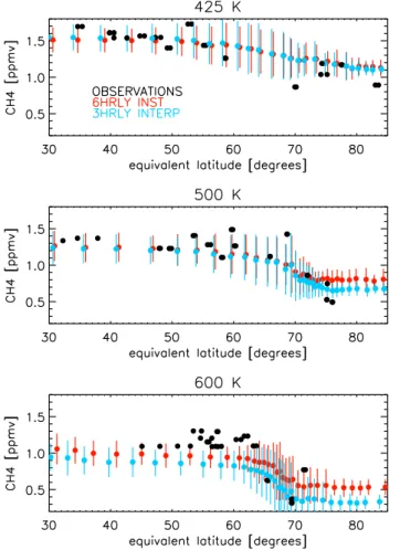
Fig. 7. Similar as Fig. 5, but with the results from the experiments
“6-hourly inst.” (blue dots) and “3-hourly interp” (red dots).
It is interesting that the modeled variability is significantly reduced in “1×1-slopes” experiment, especially in active mixing regions: close to the vortex bottom and at the vor-tex edge. This reflects the increased tracer information in the zoom region, despite the more diffusive advection scheme (see Fig. 4).
As can be seen in Fig. 7 the calculated gradients became stronger when introducing time interpolation and in partic-ular by increasing the meteorological update frequency, in line with the model results described earlier. The differences with the results from the default (“6hrly inst”) experiment in-crease with increasing potential temperature level. At 600 K the model underestimates the observations at 50–60◦N out-side the polar vortex, which is apparent in the results from all model experiments. It is also interesting that the variability of the “3hrly interp” experiment is similar to that calculated by the “6hrly inst” experiment. Since the variability calcu-lated by the “1×1-slopes” experiment is much less one may expect a stronger vortex edge gradient. However, this is not the case, as can clearly be seen in Fig. 3.
Note that even in the best model performance the calcu-lated gradient is slightly underestimated, indicating
remain-Fig. 8. Calculated latitudinal cross section of zonally average mean
age of air (years) for three different experiments: 6-hourly instan-taneous (top panel), 6-hourly interpolated (middle panel) and the 3-hourly interpolated winds (bottom panel), respectively.
ing diffusivity and/or the lack of chemistry. Although the effect of chemistry has been tested to have a negligible im-pact on methane at levels below 10 hPa in a similar model experiment (van Aalst et al., 2004), caution must be taken by treating methane as a passive tracer. Especially close to more chemically active regions of the atmosphere, i.e., the upper stratosphere outside the polar vortex. Indicative for this influence could be the slight underestimation by the model in Fig. 6 and 7 at the highest potential temperature level (600 K).
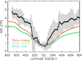
Fig. 9. Observed and calculated mean age of air for the same
ex-periments as in Fig. 8. The observations (black dots) are derived from multi-year CO2observations from the ER-2 at approximately
20 km altitude (Andrews et al., 2001). The error bars represent 2-σ standard deviation.
4.2 Mean age of air experiment
In this diagnose we evaluate the large-scale meridional cir-culation in the stratosphere by calculating the mean age of air, as described in the experimental setup section. Recently our group has performed this diagnose for a variety of model versions, including CTM and trajectory calculations (Breg-man et al., 2003; Meijer et al., 2004; Scheele et al., 2005). All these CTM calculations were performed including polar grid averaging and some of these experiments also included first-order advection. Meijer et al. (2004) found that apply-ing first-order advection has negligible impact on the mean age of air. We have performed an additional mean age of air calculation for the “1×1 slopes” experiment to examine the effect of grid resolution on the mean age. Since this diagnos-tic covers both hemispheres we were forced to use a global 1◦×1◦grid instead of a zoom region.
None of the model experiments have sofar examined the effect of time interpolation and update frequency of the winds on the mean age of air. Figure 8 shows the calculated zonally average mean age of air for the CTM experiments “6hrly inst” (top panel), “6hrly interp” (middle panel) and “3hrly interp” (bottom panel). The maximum mean age cal-culated by the “6hrly inst” experiment is around 3.5 years, which is significantly too young acocording to observations. This finding is in line with the conclusions in previous stud-ies that the meridional circulation is too fast for assimilated winds leading to too short stratospheric residence times of the air parcels (Schoeberl et al., 2002; Meijer et al., 2004; Douglass et al., 2003).
When applying time interpolation (“6hrly interp”) the re-sults improve marginally in the lower stratosphere, in agree-ment with the results from the CH4 diagnose. The air
be-Fig. 10. Observed and calculated mean age of air for the
experi-ments “3×2-slopes”, “3×2-slopes red. grid”, and “1×1-slopes”.
comes approximately 0.5 year older in the middle and upper stratosphere. However, the mean age of air is significantly older when using 3-hourly interpolated winds, with maxi-mum a mean age in the upper stratosphere close to 5 years. This result shows that increasing the update frequency im-proves the tracer transport on a hemispheric scale consider-ably.
Figure 9 shows the calculated zonally average mean age of air for the same three runs compared to observations, but now at approximately 20 km altitude. For the evaluation of the modeled mean age of air we used a compilation of CO2
and SF6 observed on board the ER-2 between 1991–1998
(Andrews et al., 2001). The calculated mean age of air from the model experiments agrees well with the observations in the tropics, but shows an underestimation in the extra-tropics with maximum ages of 3–3.6 years at 20 km altitude. Note that the mean age from the “6hrly inst” experiment is simi-lar to that calculated by Meijer et al. (2004) in their default model setup experiment.
In line with Fig. 8 the use of 3-hourly interpolated winds increases the mean age of air. The calculated meridional gra-dient of the mean age is significantly steeper than using 6-hourly winds, indicative of reduced dispersion. Neverthe-less the calculated mean age still remains about one year too young in the extra-tropical lower stratosphere. Applying time interpolation in the 6-hourly winds only yields a small improvement in the lower stratosphere.
Figure 10 shows the calculated zonally average mean age of air at 20 km altitude for three different experiments ap-plying first-order (slopes) advection. For clarity we have added the results from the experiment “3×2 slopes red. grid”, which is similar as the one used by Meijer et al. (2004). As can be seen, all experiments give very similar results. We therefore have omitted the meridional cross-section fields. Although the calculated mean tropical ages are realistically
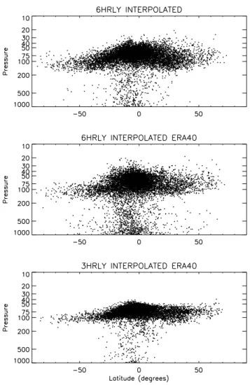
Fig. 11. The end locations of the air parcels after 50 days
back-trajectory calculations using 6-hourly interpolated winds from the operational analyses (top panel), and using 6-hourly and 3-hourly interpolated winds from re-analyses data, ERA40 (middle and bot-tom panel).
represented, the extra-tropical mean age of air is significantly too young with maxima of only 3 years(SH) and 2–2.5 years (NH). Consequently, the observed meridional gradient is un-derestimated.
There is negligible improvement when omitting the re-duced polar grid and even when increasing the model hor-izontal grid resolution to 1◦×1◦degree. These results
indi-cate little sensitivity of the mean age of air to grid resolution. This can be expected since the stratospheric tracer gradients are relatively small in these diagnostics, considerably reduc-ing the advantage of more tracer information per grid vol-ume. As pointed out by others (Hall et al., 1999; Waugh and Hall, 2002) the mean age of air diagnostics is designed to evaluate the quality of the winds.
Fig. 12. The fraction of air parcels crossing the tropopause for the
same experiments as in Fig. 11: 6-hourly interpolated winds from OD (green line), and 6-hourly (red line) and 3-hourly (blue line) interpolated winds from ERA40.
4.3 Back-trajectory experiments
Next we focus on the tropical lower stratosphere, since this is a key region for the large-scale meridional circulation. With back-trajectory calculations we calculate the dispersion of air parcels after 50 days. This time scale is much shorter than the mean age of air, but the dispersion intensity is a useful measure of the noise in DAS winds and thus indirectly relates to the mean age of air (Schoeberl et al., 2002; Scheele et al., 2005). So far we have illustrated that increasing the update frequency of the assimilated winds significantly improves the stratospheric tracer transport on a hemispheric scale. In this diagnose we examine the impact of update frequency for the 40-year re-analyses from the ECWMF (ERA40).
We examined 6-hourly and 3-hourly interpolated winds from ERA40. For comparison we added the 6-hourly inter-polated winds from the operational analyses, corresponding to our “6hrly interp” experiment. Figure 11 shows the end points of the air parcels after 50 days. The “6hrly interp” winds are considerably dispersive both horizontally and ver-tically, similar to the results from Schoeberl et al. (2002) and clearly reflects the dispersive character of assimilated winds. The middle panel shows that the ERA40 6-hourly inter-polated winds lead to somewhat more dispersion. This is well known, since winds derived by 3DVAR assimilation are more dispersive than winds from the computationally more expensive 4DVAR assimilation (Scheele et al., 2005). How-ever, the 3-hourly winds from ERA40 show much less verti-cal dispersion (lower panel in Fig. 11), even compared to the 6-hourly interpolated winds from the operational analyses. Interestingly, the horizontal dispersion is not reduced in the 3-hourly winds. In the next section we demonstrate that this may reflect real atmospheric motion rather than an indication of poor wind quality.
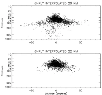
Fig. 13. The end locations of 2880 air parcels after 50 days
back-trajectory calculations using 6-hourly interpolated winds from the operational analyses, similar as in Fig. 11, using a starting altitude at the equator at an altitude of 20 km (top panel) and 22 km (bottom panel).
Figure 12 shows the air parcel dispersion more quantita-tively by the fraction of air parcels crossing the tropopause irriversibly. The larger the fraction, the more dispersive the winds. In line with Fig. 11, the 6-hourly interpolated winds from the operational analyses are less dispersive than the 6-hourly winds from ERA40. This result is similar as in Fig. 2 in Scheele et al. (2005). But now adding the results from 3-hourly ERA40 data yields a strong decrease of the fraction. It is even smaller than that calculated with the 6-hourly winds from the operational analyses.
5 Discussion
Particularly the use of 3-hourly winds results in improved stratospheric tracer distributions. It is important to note that the use of 3-hourly winds does not introduce more noise in an Eulerian frame as in most CTMs, but introduces more real variability in the wind fields. However, the most suitable up-date frequency for stratospheric tracer transport remains to be determined. This issue is directly related to the represen-tation of the winds from the GCM that provides the winds to the data assimilation system. Waugh et al. (1997) discussed different time intervals, averaging and aliasing effects but not for time frequencies of 3 h or even less. Investigating this problem is however not trivial and is subject of further study. Interestingly, the horizontal dispersion is not reduced when applying 3-hourly winds. Since the mean age of air in the tropical region is well represented, reducing the horizon-tal resolution would likely result in too old air. Although the amount of horizontal dispersion cannot be validated, useful
information can be derived from observations of the aerosols after the eruption of Mount Pinatubo. Airborne differential absorption LIDAR observations reveal a well-mixed lower stratospheric layer in the tropics and subtropics (Grant et al., 1994). The altitude of that layer is about 20 km coinciding with the initial altitude of the back trajectory calculations. The observations indicate that this layer is only about 1 to 2 kilometers thick where above a strong meridional gradi-ent is visible, represgradi-enting the sub-tropical barrier. Hence, enhanced horizontal dispersion is not necessarily an indica-tion of poor model wind quality, but may in contrast be real atmospheric transport.
To investigate this interpretation we performed an addi-tional air parcel dispersion experiment where we increased the starting altitude with 2 km to see if the model winds would also lead to reduced horizontal dispersion as the obser-vations indicate. We used the same 6-hourly winds from the operational analyses as in the top panel in Fig. 11 and started 2880 back-trajectories at the equator at 20 and 22 km altitude respectively. The results are shown in Fig. 13. The disper-sion using a starting point at 20 km is similar as in Fig. 11 top panel albeit with less trajectories. Indeed, the dispersion in particular in the horizontal, but also in the vertical direction is strongly reduced when using 22 km as starting point.
This demonstrates that the dispersive character of DAS winds in the tropical region is very sensitive to altitude and that the calculated dispersion intensity follows the observed vertical structure of the sub-tropical barrier. The strong sensi-tivity of the dispersion to altitude right at the initial altitude of the trajectory calculations questions the experimental setup applied in this study to assess air parcel dispersion. Note that this experimental setup is similar as in e.g. Schoeberl et al. (2002) and is a generally accepted diagnose.
The representation of the large-scale meridional circula-tion in the stratosphere by DAS winds may considerably im-prove when using isentropic vertical coordinates and heat-ing rates instead of vertical wind velocity or mass fluxes on pressure levels (Mahowald et al., 2002; Chipperfield, 2006). Although an isentropic coordinate seems physically more appropriate for stratospheric dynamics, a mass cor-rection needs to be performed in order to balance the di-vergence with the isentropic tendencies, which will impact the tracer distributions. This is a fundamental mass bal-ance problem that applies to both CTMs and GCMs in-dependent of the vertical coordinate system, as has been demonstrated by J¨ockel et al. (2001) and for which differ-ent mass fixers have been introduced (cf. Bregman et al., 2003; Rotman et al., 2004). When integrating over a full vertical range from the upper stratosphere to the surface, the isentropic vertical coordinate needs to be adjusted from purely isentropic to a hybrid of pressure and isentropes. So far only two models have inferred such a hybrid coordi-nate (Mahowald et al., 2002; Chipperfield, 2006), which still contain mass imbalance issues but are promising develop-ments.
Nevertheless, hybrid σ -pressure remains a practical verti-cal coordinate for global tracer modeling because of cloud presence. Radiative heating calculations are complicated in the vicinity of clouds, also aloft introducing additional un-certainty in vertical transport with isentropic coordinates.
6 Conclusions
In this study we used a 3-D CTM and a trajectory model to investigate the impact of a variety of different model config-urations and different representations of the assimilated me-teorology on stratospheric tracer transport. In particular we examined the impact of model grid resolution including the reduction of the polar grid, the diffusivity of the advection scheme, time interpolation and the update frequency of the applied assimilated winds. As diagnostics we used the CTM for CH4 transport in the Arctic polar vortex and the mean
age of air, and the trajectory model for air parcel dispersion in the tropical lower stratosphere. The CTM used ECMWF operational data only, while the trajectory model used both operational data and the ECWMF 40-year re-analyses.
The sensitivity experiments demonstrated that at least second-order moments in the advection are required for stratospheric modeling, which is well known in the model-ing community. However, a more diffusive (first-order) ad-vection yield reasonable tracer distributions when increasing the horizontal resolution to 1◦×1◦, which contrasts the
con-clusions from our previous model evaluation. The reason for this contrasting result is because in the previous model study a polar grid averaging was applied to avoid numerical prob-lems, while in this study such averaging could be avoided through iterative advection.
This study thus demonstrates the danger of the commonly applied polar model grid averaging when evaluating model grid resolution and contains an important message for other global model studies on polar tracer transport. Iterative ad-vection makes high resolution modeling feasible in the polar regions with a global CTM.
The impact of wind variability by time interpolation and in particular by increasing the update frequency affects the stratospheric CH4distribution in the polar region. Using
6-hourly time interpolated instead of instantaneous winds re-sulted in reduced cross vortex edge mixing and closer agree-ment with the observed CH4profiles inside the Arctic polar
vortex. Reducing the time interval to 3 h improves the model results even further and yield excellent agreement with the observed CH4polar vortex profiles.
The stratospheric meridional circulation is examined by diagnosing the mean residence time (age) of air in the strato-sphere. De default model version yields too young mean age of air, in agreement with previous model studies. This is a well known shortcoming of dispersive assimilated winds which enhance the stratospheric circulation. More interest-ingly is that both polar grid averaging and increased
horizon-tal resolution have negligible impact on the mean age of air in contrast to the findings in the polar region. Apparently, the small stratospheric tracer gradients make this diagnose insensitive to the amount of tracer information per grid cell volume.
The mean age of air is more sensitive to wind variabil-ity. It becomes significantly older in the extra-tropical strato-sphere when applying 3-hourly instead of 6-hourly interpo-lated winds. The mean age is less sensitive to time inter-polation and is particularly noticeable in the middle and up-per stratosphere where it becomes 0.5 year older compared to the default model experiment. The tropical mean age of air shows excellent agreement with observations, although the extra-tropical lower stratospheric mean age remains too young with about one year.
The back-trajectory experiments show that the 6-hourly re-analyses contains more dispersion than the 6-hourly opera-tional analyses as is expected when applying 3DVAR assim-ilation. In line with the findings from the mean age of air di-agnostic, the use of 3-hourly winds significantly reduces the vertical dispersion in the tropical lower stratosphere and the re-analyses data even contains less vertical dispersion than the winds produced by the 6-hourly interpolated operational analyses.
The horizontal dispersion in particular remains relatively strong, even when applying 3-hourly winds. However, it is important to note that strong horizontal transport is ob-served around 20 km altitude in the tropics and subtropics, so that calculated enhanced horizontal dispersion is not nec-essarily an indication of poor wind quality. Starting the back-trajectory calculations only 2 km higher the dispersion is considerably reduced, coinciding with the observed verti-cal structure of the sub-tropiverti-cal barrier. Hence, the dispersion calculations using the current experimental setup should be interpreted with great care.
For models using vertical hybrid sigma-pressure coordi-nates recent new insights in the implementation of DAS winds in CTMs has improved the stratospheric tracer rep-resentation considerably, both in the polar region as on a hemispheric scale. It is recommended not to use a reduc-tion of the polar grid (either through grid cell merging or by wind averaging). We also recommend applying time interpo-lation instead of using instantaneous winds. In line with the findings from Legras et al. (2005) it is also recommended to apply 3-hourly instead of the commonly used 6-hourly up-date interval. These results in combination with expected improvements in the data assimilation procedures give new perspectives for long-term tracer integrations using assimi-lated winds.
Acknowledgements. Part of this work is funded by the European
Commission, through the project TOwards the Prediction of strato-spheric OZone (TOPOZ) III, under contract no. EVK2-CT-2001-00102, the project Stratospheric-Climate Links with Emphasis on the Upper Troposphere and Lower Stratosphere (SCOUT), and the National (Netherlands) User Support Programme (GO)2. We
thank M. Krol and A. Segers for computational support and useful discussions. We are also grateful to A. Stohl and one anonymous reviewer for their valuable comments.
Edited by: B. K¨archer
References
Andrews, A., Boering, K., Daube, B., Wofsy, S., Loewenstein, M., Jost, H., Podolske, J., Webster, C., Herman, R., Scott, D., Flesh, G., Moyer, E., Elkins, J., Dutton, G., Hurst, D., Moore, F., Ray, E., Romanshkin, P., and Strahan, S.: Mean ages of stratospheric air derived from in situ observations of CO2, CH4, and N2O, J.
Geophys. Res., 106, 32 295–32 314, 2001.
Berthet, G., Huret, N., Lef´evre, F., Moreau, G., Robert, C., Chartier, M., Catoire, V., Barret, B., Pisso, I., and Pomathiod, L.: On the ability of chemical transport models to simulate the vertical structure of the N2O, NO2and HNO3species in the mid-latitude
stratosphere, Atmos. Chem. Phys., 6, 1599–1609, 2006, http://www.atmos-chem-phys.net/6/1599/2006/.
Bregman, A., Krol, M., Teyss`edre, H., Norton, W., Chipperfield, M., Pitari, G., Sundet, J., and Lelieveld, J.: Chemistry-transport model comparison with ozone observations in the midlatitude lowermost stratosphere, J. Geophys. Res., 106, 17 479–17 496, 2001.
Bregman, A., Wang, P.-H., and Lelieveld, J.: Chemical ozone loss in the tropopause region on subvisible ice clouds, calcu-lated with a chemistry-transport model, J. Geophys. Res., 107, doi:10.1029/2001JD000761, 2002.
Bregman, B., Segers, A., Krol, M., Meijer, E., and van Velthoven, P.: On the use of mass-conserving wind fields in chemistry-transport models, Atmos. Chem. Phys., 3, 447–457, 2003, http://www.atmos-chem-phys.net/3/447/2003/.
Chipperfield, M.: New version of the TOMCAT/SLIMCAT off-line chemical transport model, Q. J. R. Meteorol. Soc., 132, 1179– 1203, doi:10.1256/qj.05.51, 2006.
Dentener, F., Feichter, J., and Jeuken, A.: Simulation of the trans-port of Rn222using on-line and off-line global models at differ-ent horizontal resolutions: A detailed comparison with measure-ments, Tellus, 51, 573–602, 1999.
Douglass, A., Schoeberl, M. R., Rood, R. B., and Pawson, S.: Eval-uation of transport in the lower tropical stratosphere in a global chemistry and transport model, J. Geophys. Res., 108, 4259, doi:10.1029/2002JD002696, 2003.
Garcelon, S., Gardiner, T., Hansford, G., Harris, N., Howieson, I., Jones, R., McIntyre, J., Pyle, J., Robinson, J., Swann, N., and Woods, P.: Investigation of CH4and CFC-11 vertical profiels in
the Arctic vortex during the SOLVE/THESEO 2000 campaign, in Proceedings of the general Assembly, Nice, European Geo-phyisical Society, 2002.
Grant, W., Browell, E., Fishman, J., Brackett, V., Veiga, R., Nganga, D., Minga, A., Cros, B., Butler, C., Fenn, M., Long, C., and Stowe, L.: Aerosol-associated changes in tropical stratospheric ozone following the eruption of Mount Pinatubo, J. Geophys. Res., 99, 8197–8211, 1994.
Hadjinicolaou, P. and Pyle, J.: The recent turnaround in stratospheric ozone over northern middle latitudes: a dy-namical modeling perspective, Geophys. Res. Lett., 32, doi:10.1029/2005GL022476, 2005.
Hall, T. and Plumb, R.: Age as a diagnostic of stratospheric trans-port, J. Geophys. Res., 99, 1059–1070, 1994.
Hall, T., Waugh, D., Boering, K., and Plumb, R.: Evaluation of transport in stratospheric models, J. Geophys. Res., 104, 18 815– 18 839, 1999.
Heimann, M.: The Global Atmospheric Tracer Model TM2, Tech. Rep. 10, DRKZ-Hamburg, 1995.
Heimann, M. and Keeling, C.: A three-dimensional model of atmo-spheric CO2transport based on observed winds: 2: Model
de-scription and simulated tracer experiments, Geophys. Mon., 55, 237–275, 1989.
Holton, J., Haynes, P., McIntyre, M., Douglass, A., and Rood, R.: Stratosphere troposphere exchange, Rev. Geophys., 33, 403–439, 1995.
Houweling, S., Dentener, F., and Lelieveld, J.: The impact of non-methane hydrocarbon compounds on tropospheric photochem-istry, J. Geophys. Res., 103, 10 673–10 696, 1998.
J¨ockel, P., von Kuhlmann, R., Lawrence, M., Steil, B., Bren-ninkmeijer, C., Crutzen, P., Rasch, P., and Eaton, B.: On a funda-mental problem in implementing flux-form advection schemes for tracer transport in 3-dimensional general circulation and chemistry transport models, Q. J. R. Meteorol. Soc., 127, 1035– 1052, 2001.
Krol, M., Houweling, S., Bregman, B., van den Broek, M., Segers, A., van Velthoven, P., Peters, W., Dentener, F., and Bergamaschi, P.: TM5, a global two-way nested chemistry transport zoom model: algorithm and applications, Atmos. Chem. Phys., 5, 417– 432, 2005,
http://www.atmos-chem-phys.net/5/417/2005/.
Laat, A., Landgraf, J., Aben, I., Hasekamp, O., and Bregman, B.: Assimilated winds for global modelling: evaluation with space- and balloon-borne ozone observations, J. Geophys. Res., in press, 2006.
Legras, B., Pisso, I., Berthet, G., and Lef´evre, F.: Variability of the Lagrangian turbulent diffusion in the lower stratosphere, Atmos. Chem. Phys., 5, 1605–1622, 2005,
http://www.atmos-chem-phys.net/5/1605/2005/.
Mahowald, M., Plumb, R. A., Rasch, P. J., del Corral, J., Sassi, F., and Heres, W.: Stratospheric transport in a three-dimensional isentropic coordinate model, J. Geophys. Res., 107, doi:10.1029/2001JD001313, 2002.
Manney, G., Allen, D., Kr¨uger, K., Naujokat, B., Santee, M., Sabutis, J., Pawson, S., Swinbank, R., Randall, C., Simmons, A. J., and Long, G.: Diagnosic comparison of meteorological analyses during the 2002 Antarctic winter, J. Atmos. Sci., 133, 1261–1278, 2005.
Manson, A., Meek, C., Koshyk, J., Franke, S., Fritts, D., Riggin, D., Hall, C., Hocking, W., MacDougall, J., Igarashi, K., and Vincent, R.: Gravity wave activity and dynamical effects in the middle at-mosphere (60–90 km): observations from an MF/MLT radar net-work, and results from the Canadian Middle Atmosphere Model (CMAM), J. Atmos. Solar-Terr. Phys., 64, 65–90, 2002. Marchand, M., Godin, S., Hauchecorne, A., Lef´evre, F., and
Chip-perfield, M.: Influence of polar ozone loss on northern midlati-tude regions estimated by a high-resolution chemistry transport model during winter 1999/2000, J. Geophys. Res., 108, 8326, doi:10.1029/2001JD000906, 2003.
Meijer, E., Bregman, B., and van Velthoven, P.: The influence of data assimilation on the age of air calculated with a global
chemistry-transport model using ECMWF winds, Geophys. Res. Lett., 31, doi:10.102/2004/GL021158, 2004.
Noije, T. P. C., Eskes, H. J., van Weele, M., and van Velthoven, P. F. J.: Implications of the enhanced Brewer-Dobson circula-tion in European Centre for Medium-Range Weather Forecasts reanalysis ERA-40 for the stratosphere-troposphere exchange of ozone in global chemistry transport models, J. Geophys. Res., 109, doi:10.1029/2004JD004586, 2004.
Peters, W., Krol, M. C., Dentener, F. J., and Lelieveld, J.: Identifi-cation of an El Ni˜no-Southern Oscillation signal in a multiyear global simulation of tropospheric ozone, J. Geophys. Res., 106, 10 389–10 402, 2001.
Polavarapu, S., Ren, S., Rochon, Y., Sankey, D., Ek, N., Koshyk, J., and Tarasick, D.: Data assimilation with the Canadian Middle Atmosphere Model, Appl. Opt., 43, 77–100, 2005.
Prather, M.: Numerical advection by conservation of second-order moments, J. Geophys. Res., 91, 6671–6681, 1986.
Randel, W., Wu, F., III, J. R., Roche, A., and Waters, J. W.: Sea-sonal cycles and QBO variations in stratospheric CH4and H2O observed in UARS HALOE data, J. Atmos. Sci., 55, 163–185, 1998.
Randel, W., Fleming, E., Geller, M., Gelman, M., Hamilton, K., Karoly, D., Ortland, D., Pawson, S., Swinbank, R., Udelhofen, P., Wu, F., Baldwin, M., Chanin, M.-L., Keckhut, P., Simmons, A., and Wu, D.: The SPARC intercomparison of Middle Atmosphere Climatologies, Tech. Rep. 20, SPARC newsletter, 2003. Rotman, D., Atherton, C., Bergmann, D., Cameron-Smith, P.,
Chuang, C., Connell, P., Dignon, J., Franz, A., Grant, K., Kinni-son, D., Molenkamp, C., Proctor, D., and Tannahill, J.: IMPACT, the LLNL 3-D global atmospheric chemical transport model for the combined troposphere and stratosphere: Model description and analysis of ozone and other trace gases, J. Geophys. Res., 109, doi:10.1029/2003JD003155, 2004.
Russel, G. and Lerner, J.: A new finite-differencing scheme for the tracer transport equation, J. Appl. Meteorol., 20, 1483–1498, 1981.
Russel-III, J., Gordley, L., Park, J., Drayson, S., Hesketh, D., Ci-cerone, R., Tuck, A., Frederick, J., Harries, J., and Crutzen, P.: The Halogen Occultation Experiment, J. Geophys. Res., 98, 10 777–10 797, 1993.
Scheele, R., Siegmund, P., and van Velthoven, P.: Stratospheric age of air computed with trajectories based on various 3-D-Var and 4-D-Var data sets, Atmos. Chem. Phys., 5, 1–7, 2005,
http://www.atmos-chem-phys.net/5/1/2005/.
Schoeberl, M., Douglass, A., Zhu, Z., and Pawson, S.: A com-parison of the lower stratospheric age-spectra, derived from a General Circulation Model and two data assimilation systems, J. Geophys. Res., 108, 4113, doi:10.1029/2002JD002652, 2002. Searle, K., Chipperfield, M., Bekkie, S., and Pyle, J.: The impact of spatial averaging on calculated polar ozone loss, 1, Model exper-iments, J. Geophys. Res., 103, 25 397–25 408, 1998.
Segers, A., van Velthoven, P., Bregman, B., and Krol, M.: On the computation of mass fluxes for Eulerian transport models from spectral meteorological fields, in: Proceedings of the 2002 Inter-national Conference on Computational Science, Lecture Notes in Computer Science (LNCS), Springer Verlag, 2002.
Shepherd, T., Koshyk, J., and Ngan, K.: On the nature of large-scale mixing in the stratosphere and mesosphere, J. Geophys. Res., 105, 12 433–12 446, 2000.
Simmons, A., Hortal, M., Kelly, G., McNally, A., Untch, A., and Uppala, S.: ECMWF analyses and forecasts of stratospheric win-ter polar vortex breakup: September 2002 in the Southern Hemi-sphere and related events, J. Atmos. Sci., 62, 668–689, 2005. Stohl, A., Eckhart, S., Forster, C., James, P., Spichtinger, N., and
Seibert, P.: A replacment of simple back trajectory calculations in the interpretation of atmospheric trace gas substance measure-ments, Atmos. Environ., 36, 4635–4648, 2002.
Stohl, A., Cooper, O., and James, P.: A cuationary note on the use of meteorological analysis data for quantifying atmospheric mix-ing, J. Atmos. Sci., 61, 1446–1453, 2004.
Strahan, S. E. and Polansky, B. C.: Meterological implementation issues in chemistry and transport models, Atmos. Phys. Chem., 6, 2895–2910, 2006.
Tan, D., Haynes, P. H., MacKenzie, A. R., and Pyle, J. A.: Effects of fluid-dynamical stirring and mixing on the deactivation of strato-spheric chlorine, J. Geophys. Res., 103, 1585–1606, 1998. Tan, W., Geller, M. A., Pawson, S., and da Silva, A.: A
case study of excessive subtropical transport in the strato-sphere of a data assimilation system, J. Geophys. Res., 109, doi:10.1029/2003JD004057, 2004.
Toon, G., Blavier, J.-F., Sen, B., Margitan, J., Webster, C., May, R., Fahey, D., Gao, R., Negro, L. D., Proffit, M., Elkins, J., Ro-mashkin, P., Hurst, D., Oltmans, S., Atlas, E., Schauffler, S., Flocke, F., Bui, T., Stimpfle, R., Boone, G., Voss, P., and Cohen, R.: Comparison of MkIV balloon and ER-2 aircraft measure-ments of atmospheric trace gases, J. Geophys. Res., 104, 26 779– 26 790, 1999.
van Aalst, M., van den Broek, M., Bregman, A., Br¨uhl, C., Steil, B., Toon, G., Garcelon, S., Hansford, G., Jones, R., Gardiner, T., Roelofs, G., Lelieveld, J., and Crutzen, P.: Tracer transport in the 1999/2000 Arctic polar vortex comparison of nudged GCM runs with observations, Atmos. Chem. Phys., 4, 81–93, 2004, http://www.atmos-chem-phys.net/4/81/2004/.
Van den Broek, M., Bregman, A., and Lelieveld, J.: Model study of stratospheric chlorine and ozone loss during the 1996/1997 winter, J. Geophys. Res., 105, 28 961–28 977, 2000.
van den Broek, M., van Aalst, M., Bregman, A., Krol, M., Lelieveld, J., Toon, G., Garcelon, S., Hansford, G., Jones, R., and Gardiner, T.: The impact of model grid zooming on tracer transport in the 1999/2000 Arctic polar vortex, Atmos. Chem. Phys., 3, 1833–1847, 2003,
http://www.atmos-chem-phys.net/3/1833/2003/.
Waugh, D. and Hall, T.: Age of stratospheric air: the-ory, observations, and models, Rev. Geophys., 40(4), doi:10.1029/2000RG000101, 2002.
Waugh, D., Hall, T. M., Randel, W. J., Rasch, P. J., Boville, B. A., Boering, K. A., Wofsy, S. C., Daube, B. C., Elkins, J. W., Fa-hey, D. W., Dutton, G. S., and Volk, C. M.: Three-dimensional simulations of long-lived tracers using winds from MACCM2, J. Geophys. Res., 102, doi:10.1029/97JD00793, 1997.
Wild, O., Sundet, J., Prather, M., Isaksen, I., Akimoto, H., Brow-ell, E., and Oltmans, S.: CTM ozone simulations for spring 2001 iver the western Pacific: comparisons with TRACE-P li-dar, ozone sondes and TOMS columns, J. Geophys. Res., 109, doi:10.1029/2003JD004041, 2003.