HAL Id: hal-00318091
https://hal.archives-ouvertes.fr/hal-00318091
Submitted on 3 Jul 2006
HAL is a multi-disciplinary open access
archive for the deposit and dissemination of
sci-entific research documents, whether they are
pub-lished or not. The documents may come from
teaching and research institutions in France or
abroad, or from public or private research centers.
L’archive ouverte pluridisciplinaire HAL, est
destinée au dépôt et à la diffusion de documents
scientifiques de niveau recherche, publiés ou non,
émanant des établissements d’enseignement et de
recherche français ou étrangers, des laboratoires
publics ou privés.
Thermally driven circulation in a region of complex
topography: comparison of wind-profiling radar
measurements and MM5 numerical predictions
L. Bianco, B. Tomassetti, E. Coppola, A. Fracassi, M. Verdecchia, G. Visconti
To cite this version:
L. Bianco, B. Tomassetti, E. Coppola, A. Fracassi, M. Verdecchia, et al.. Thermally driven circulation
in a region of complex topography: comparison of wind-profiling radar measurements and MM5
numerical predictions. Annales Geophysicae, European Geosciences Union, 2006, 24 (6),
pp.1537-1549. �hal-00318091�
comparison of wind-profiling radar measurements and MM5
numerical predictions
L. Bianco, B. Tomassetti, E. Coppola, A. Fracassi, M. Verdecchia, and G. Visconti Centre of Excellence – CETEMPS, University of L’Aquila, L’Aquila, Italy
Received: 14 October 2005 – Revised: 18 April 2006 – Accepted: 17 May 2006 – Published: 3 July 2006
Abstract. The diurnal variation of regional wind patterns in the complex terrain of Central Italy was investigated for sum-mer fair-weather conditions and winter time periods using a radar wind profiler. The profiler is located on a site where in-teraction between the complex topography and land-surface produces a variety of thermally and dynamically driven wind systems. The observational data set, collected for a period of one year, was used first to describe the diurnal evolution of thermal driven winds, second to validate the Mesoscale Model 5 (MM5) that is a three-dimensional numerical model. This type of analysis was focused on the near-surface wind observation, since thermally driven winds occur in the lower atmosphere. According to the valley wind theory expecta-tions, the site – located on the left sidewall of the valley (looking up valley) – experiences a clockwise turning with time. Same characteristics in the behavior were established in both the experimental and numerical results.
Because the thermally driven flows can have some depth and may be influenced mainly by model errors, as a third step the analysis focuses on a subset of cases to explore four different MM5 Planetary Boundary Layer (PBL) parameter-izations. The reason is to test how the results are sensitive to the selected PBL parameterization, and to identify the better parameterization if it is possible. For this purpose we anal-ysed the MM5 output for the whole PBL levels. The chosen PBL parameterizations are: 1) Gayno-Seaman; 2) Medium-Range Forecast; 3) Mellor-Yamada scheme as used in the ETA model; and 4) Blackadar.
Keywords. Atmospheric composition and structure (Evolu-tion of the atmosphere) – Meteorology and atmospheric dy-namics (Convective processes; Turbulence)
Correspondence to: L. Bianco
(laura.bianco@aquila.infn.it)
1 Introduction
Understanding of mountain phenomena has been an area of active research for many years and it is a subject of large interest to weather forecasters, research meteorologists, air quality scientists, and numerical modelers. The behavior of mesoscale wind patterns within complex mountain and valley terrains has been described with considerable detail early in the last century by Wagner (1938), and later by De-fant (1951). More recently, a complete description of lo-cal circulation induced by complex topography can be found in Atkinson (1981), while mesoscale modeling of terrain-induced systems are extensively discussed in Pielke (2002). The basic theory for thermal flows involves two types of wind systems: slope winds and mountain-valley winds. Essen-tially, in the morning, the heating of the slope at the sides of a valley produces a pressure gradient favorable to ups-lope wind acceleration. Heating persists and upsups-lope winds draw air from the interior of the valley; this air is replaced by warmer air, presumably from above. The warming pro-duces a pressure drop in the valley relative to the plains into which the valley opens. A wind begins to blow up the val-ley toward the mountain, and up-valval-ley winds persist for the rest of the afternoon. At night the opposite occurs: cooling at the surface produces down-slope “drainage” winds and ul-timately down-valley “mountain” winds. The interaction of these wind systems creates complex flow patterns that are part of the everyday winds in complex terrain: the superposi-tion of valley and slope winds produces a clockwise diurnal rotation on the left (when looking up) sidewall of a valley and counterclockwise diurnal rotations on the right one (Hawkes, 1947; Whiteman 1990).
Many studies have been conducted to understand the ther-mally and dynamically wind systems in regions of complex topography (Stewart et al., 2002; Whiteman et al., 1999; Horel et al., 2002). The difficulty in reaching a clear under-standing of the way topography influences this wind behavior
1538 L. Bianco et al.: Thermally driven circulation in a region of complex topography
Figures:
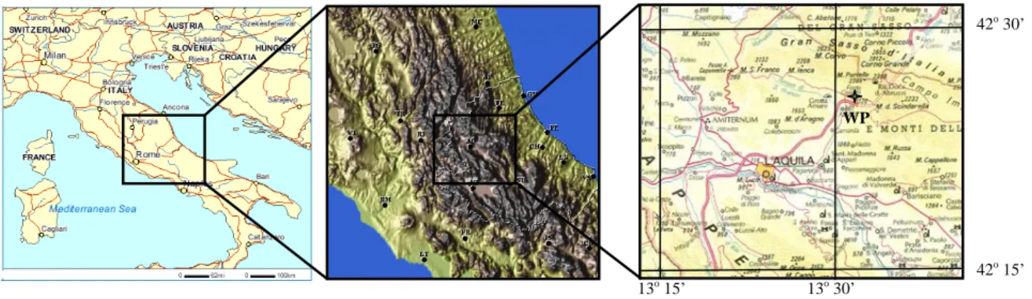
Page 1, Fig. 1. In the right panel the letters WP are not visible.
Please, substitute the figure with the following:
13o 15’ 13o 30’
42o 30’
42o 15’ WP
Label of Fig. 3, line 3: replace: “Altitudes range from 60 to 2800 m.” With: “Altitudes
range from 600 to 2800 m.”
Abstract:
Page 1, column 1, and line 19: Replace: “…and maybe influenced mainly by model
errors, as a second….” With: “…and maybe influenced mainly by model errors, as a
third….”
Introduction:
Page 2, column 1, and line 5: Replace: “several day and low cloudiness.” With: “several
days and low cloudiness.”
Page 2, column 2, and line 17: Replace: “… (22 May 2002-22 May 2003) and it gives us
the opportunity….” With: “…(22 May 2002-22 May 2003) giving us the opportunity….”
Page 3, column 3, and line 1: Replace: “…circulation in an area of complex
topography,…” With: “…circulation in the area of interest,…”
Paragraph 2:
Page 4, column 1, and line7: Replace: “… site is inland and placed at the southeast
foothills…” With: “… site is inland and placed at the southwest foothills…”
Paragraph 3:
Page 6, column 2, and line 1: Replace: “…u and w wind components…” With: “…u and
v wind components”
Paragraph 4:
Page 9, Section 4.1.2, line 8: Replace: “… similar to the…” With: “… similarly to the…”
Paragraph 5:
Page 11, line 5: Replace: “… placed at the southeast…” With “… placed at the
southwest…”
Fig. 1. Map of the Assergi site. The altitude of the region in the right panel ranges between 700 and 2912 m ASL. In the right panel the wind profiler (WP) location is denoted with the star.
is due to the fact that there is not one but a variety of mech-anisms in different terrain structures. Moreover, to force a thermal driven circulation, the site has to experience fair weather conditions, with a constant synoptic scale flow for several days and low cloudiness.
The aim of this paper is first to describe the diurnal evo-lution of thermal driven winds during summer fair-weather conditions and winter time periods, in a region of partic-ular interest. Second, the purpose of the work is to vali-date the Mesoscale Model 5 (MM5) from the Pennsylvania State University/National Center for Atmospheric Research (PSU/NCAR) in the same area. The region is located in Cen-tral Italy, where winds are strongly influenced by complex topography, strong solar radiation, large diurnal variation in air temperature, dry air, dry soil, and land-surface contrasts. All these forcing produce a variety of thermal and dynami-cal driven wind systems that will be analyzed in detail in this paper. The fair-weather conditions are chosen because when large-scale flows are usually weak and skies are clear, spatial variations in surface heating and cooling – arising from com-plex topography and land-surface contrasts – produce ther-mally driven flows that dominate local circulation pattern.
The motivation of the work is to improve our knowledge of local and regional airflow patterns which develop in com-plex terrain and to investigate the different surface effects on airflow, their interaction, and the individual local wind com-ponents, such as the mountain/valley wind circulations. The development of valley and mountain winds at this site on a daily basis is analysed and compared with the type of circu-lation suggested by the theory mentioned above.
The possibility of realistically reproducing the thermally driven circulation at a horizontal resolution of few kilome-ters by MM5 is investigated too and our analysis is per-formed for a whole year rather than for few individual cases (Zhong and Fast, 2002). In a previous work (Tomassetti et al., 2003) the operational version of MM5 was used to sim-ulate possible climatic changes induced by land-use modi-fication. Tomassetti et al. (2003) showed that this model is
able to reproduce expected hydrometeorological effects in-duced by the drainage of Fucino Lake in an area close to the site analyzed in the current paper, and in the same paper the sensitivity of the model to the land use change has also been tested. An important goal is to show how the diurnal vari-ation of near-surface thermally driven wind is realistically simulated by MM5.
For this study we used meteorological observations ac-quired by a radar wind profiler located at the considered site and we compare them with the MM5 model simulations per-formed at the Centre of Excellence for the Integration of Remote Sensing Techniques and Numerical Modeling for the Forecast of Severe Weather (CETEMPS) – University of L’Aquila, Italy.
The wind profiler data have been collected for one year (22 May 2002–22 May 2003) giving us the opportunity to study the local wind regime. We first concentrate on examin-ing the temporal near-surface evolution of the wind fields and their consistency at a given time of the day, for both the wind profiler measurements and the MM5 predictions. Moreover, since the thermally driven flows can have some depth and may be influenced by model errors, we extended our analy-sis to include the whole PBL. In this last analyanaly-sis we focused on a subset of cases for investigating the effects of four dif-ferent PBL parameterizations: 1) Gayno-Seaman (thereafter GAYNO); 2) Medium-Range Forecast (thereafter MRF); 3) ETA; and 4) Blackadar (thereafter BLAC). We wanted to test how the results were sensitive to the chosen PBL parameteri-zation and to identify the parameteriparameteri-zation that works better. The large amount of time needed to run the model did not al-low us to reproduce this type of analysis for the entire data set of experimental data, but we had to choose a subset of cases to consider in our simulations. The subset of cases (18 fair-weather days) was selected in the summer period, when the thermally driven circulation was well defined.
Fig. 2. Picture of the Assergi site. The wind profiler is located on the top of one building of the National Laboratory of Gran Sasso (LNGS), as visible in the picture, at an altitude of 981 m ASL. The picture is taken looking toward the North – North-East direction.
33
Fig. 2. Picture of the Assergi site. The wind profiler is located on the top of one building of the National Laboratory of Gran Sasso (LNGS), as visible in the picture, at an altitude of 981 m ASL. The picture is taken looking toward the north–northeast direction.
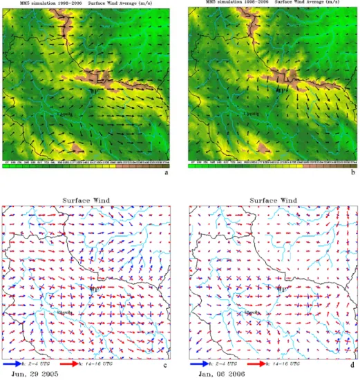
Fig. 3. Analysis of surface winds at the Assergi area carried out using long MM5 time series (years 1998-2005). Panel a) is relative to summertime analysis, panel b) to wintertime analysis. Wind arrows are show at each MM5 grid point, and grid resolution is 3 km. The Wind Profiler location is denoted with WP. Altitudes range from 60 to 2800 meters. Panels c) and d) show the daily wind rotation for two clear sky situations, panel c) for a summer case and panel d) for a winter case. Blue arrows represent the average wind direction and intensity in the interval between 2 - 4 UTC, red arrows in the interval between 14 -16 UTC.
Fig. 3. Analysis of surface winds at the Assergi area carried out using long MM5 time series (years 1998-2005). Panel (a) is relative to summertime analysis, panel (b) to wintertime analysis. Wind arrows are shown at each MM5 grid point, and grid resolution is 3 km. The wind profiler location is denoted with WP. Altitudes range from 600 to 2800 m. Panels (c) and (d) show the daily wind rotation for two clear-sky situations, panel (c) for a summer case and panel (d) for a winter case. Blue arrows represent the average wind direction and intensity in the interval between 02:00–04:00 UTC, red arrows in the interval between 14:00–16:00 UTC.
Section 2 introduces the site under study, the instrument used to collect data, the data processing, and the analysis pro-cedures. Section 3 presents the MM5 model principles. Sec-tion 4 is divided in two subsecSec-tions. SecSec-tion 4.1 shows the
re-sults of our analysis of the near-surface thermally driven cir-culation in the area of interest, and the comparison between the wind profiler measurements and the numerical model pre-dictions. In Sect. 4.2 we test the MM5 sensitivity against four
1540 L. Bianco et al.: Thermally driven circulation in a region of complex topography
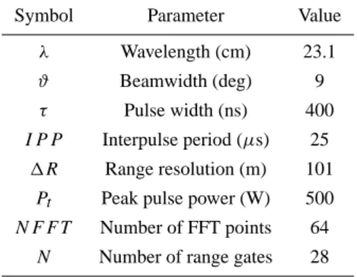
Table 1. Parameters set for the wind profiler.
Symbol Parameter Value
λ Wavelength (cm) 23.1
ϑ Beamwidth (deg) 9
τ Pulse width (ns) 400
I P P Interpulse period (µs) 25
1R Range resolution (m) 101
Pt Peak pulse power (W) 500
N F F T Number of FFT points 64
N Number of range gates 28
different PBL parameterizations, comparing the predictions of the model with the wind profiler observations. Finally, Sect. 5 presents a summary of the results.
2 Site under study, instrument and data analysis proce-dures
The region we investigated was selected because it has a long period of continuous observations, throughout an entire year, and can give an ideal data set to study a typical thermally driven wind system in Central Italy. The area is located in Assergi (L’Aquila, Italy), at latitude 42.50◦N and longitude 13.50◦E, and 981 m Above Sea Level (ASL) of altitude. The site is inland and placed at the southwest foothills of the Gran Sasso peak (2912 m ASL); it has dry air, dry soil, and shows large diurnal variation in air temperature. A map of the site is shown in Fig. 1 and a picture of the location of the wind profiler is presented in Fig. 2. The picture is taken looking toward the north–northeast direction.
Using MM5, we estimated a typical diurnal temperature range at the radar location from –5 to 2◦C during the coldest month (January) and from 11 to 21◦C during the warmest month (July).
The topography is of critical importance for the wind flow pattern present at the site. The wind profiler sees the reg-ular slope of the mountain to its north–northeast direction while the valley is evident to its south–southwest side. There-fore, winds with a northeasterly component are down-slope, or down-valley, and those with a southwesterly component are up-slope, or up-valley. Much of the area (up to the tree line on the side of the mountain) consists of uniform vege-tation and small and sparse buildings. During the summer-time the site is well exposed to the solar radiation throughout the whole daytime. Figures 3c and d show typical clear sky cases for summer and wintertime. In both maps we report the averaged circulation near surface as simulated by the MM5 model. The rotation of the surface wind from north-east to south-west from nighttime to daytime is evident.
Data from a 1290 MHz wind profiler were used for this study. The instrument is a five-beam radar wind profiling manufactured by Radian Corporation (now Vaisala). The radar samples the atmosphere from 101 m to 2833 m ASL in the vertical direction, with a 101- m resolution. Data col-lected in the period 22 May 2002–22 May 2003 at Assergi (L’Aquila) are utilized in the analysis. Some of the character-istics of the wind profiler used in this work are summarized in Table 1.
The first focus of this paper is the analysis of near-surface wind observation, since thermally driven winds occur in the low atmosphere. For this reason, the first measurements’ height is used in the comparison with the numerical model prediction results.
The summer months of May, June, July, August, and September were extracted from the period under analysis and considered in the summertime analysis, while the remaining data were included in the wintertime analysis. In the set of data we selected the fair-weather days following the defini-tion in Whiteman et al. (1999): for a particular day, skies were considered clear to partly cloudy if the observed to-tal daily solar radiation was larger than 64% of the theoret-ical extraterrestrial solar radiation power, as computed by a numerical model (following Whiteman and Allwine, 1986). They found that on clear days, the daily incoming radiation was about 80% of the daily extraterrestrial total (top of the atmosphere incoming short-wave radiation). As a conse-quence, the 64% cutoff, in fact, defined partly cloudy days as those days receiving 80% or more of the clear-day radiation total. Solar radiation observations were provided by ARSSA (Regional Agency for Agriculture Service). The sensor used for our analysis is the closest one to the site of interest and belongs to a regional network of stations and is located at latitude 42.20◦N and longitude 13.22◦E, and an altitude of 955 m (ASL).
Following Whiteman et al. (1999), the analysis on the radar wind profiler data was performed computing a median fair-weather wind, for each of the 24 h of the day, by aver-aging hourly wind values. This procedure was performed on the winds acquired by the profiler at the lowest height, for each hour of the day and for all the fair-weather hours during the experimental period of interest (giving a total of 44 days for the summer analysis and 112 days for the winter one). To better interpret these computed hourly vector winds, the vari-ability of the winds used in computing the vector average was determined using wind persistence, which was introduced by Panofsky and Brier (1965) and is defined as the ratio of the vector mean wind speed and the scalar wind speed. This ra-tio is equal to 1 when all days have identical wind direcra-tions at the considered hour, and is less than 1 when the wind di-rection at a particular hour varies from day to day. In the ex-treme situation of the ratio being equal to 0, the wind persis-tence tells us that, for that particular hour, the wind is equally likely from all directions or it blows half the time from one direction and half the time from the opposite direction.
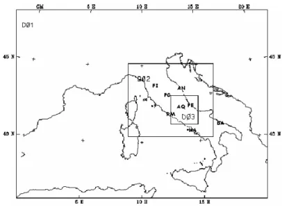
Fig. 4. Triple nested domain used for the simulations.
35
Fig. 4. Triple nested domain used for the simulations.
Fig. 5. a) Diurnal cycle of the near-surface wind vector of the “representative day”, during summer season at the Assergi site, as observed by the radar wind profiler. b) Diurnal variation of wind persistence relative to the wind vector in the upper panel. (GMT = LT - 1).
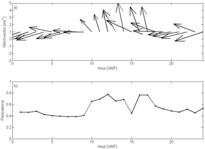
Fig. 5. (a) Diurnal cycle of the near-surface wind vector of the “representative day”, during summer season at the Assergi site, as observed by the radar wind profiler. ( b) Diurnal variation of wind persistence relative to the wind vector in the upper panel (GMT = LT–1).
3 Mesoscale Model 5 (MM5)
The meteorological model used in this work is the non-hydrostatic version of the NCAR/Pennsylvania State Uni-versity Mesoscale Model MM5 (Dudhia 1993; Grell et al., 1994). MM5 is a primitive equation, σ vertical coordinate model used by a broad research community for a variety of applications. It also includes a number of different options of physical parameterizations.
In the framework of the CETEMPS activities, MM5 has been operational since 1998; for the daily simulations the Kain-Fritsch cumulus cloud scheme (Kain and Fritsch, 1990), along with an explicit cloud water/ice scheme (Grell et al., 1994) is used. Radiative transfer is represented by the
simplified scheme described in Grell et al. (1994) and bound-ary layer physics is described by the MRF scheme (Troen and Mahrt, 1986). For land surface processes the standard MM5 scheme is used, in which the surface temperature is calcu-lated via a force-restore method and evaporation is computed using a fixed moisture availability parameter (the ratio of ac-tual to potential evaporation) dependent on the surface vege-tation type. The operational model uses 24 unevenly spaced
σlevels. All the simulations are driven by the ECMWF (Eu-ropean Centre for Medium-range Weather Forecast) global analyses; forecast and boundary conditions are upgraded ev-ery 6 h and no data assimilation is done during the opera-tional runs. Figure 4 shows the model triple nested domain used in the experiments. The outer domain covers Italy and
1542 L. Bianco et al.: Thermally driven circulation in a region of complex topography
Fig. 6. a) Diurnal cycle of the near-surface wind vector of the “representative day”, during summer season at the Assergi site, as predicted by the Mesoscale Model 5. b) Diurnal variation of wind persistence relative to the wind vector in the upper panel.
37
Fig. 6. (a) Diurnal cycle of the near-surface wind vector of the “representative day”, during the summer season at the Assergi site, as predicted by the Mesoscale Model 5. (b) Diurnal variation of wind persistence relative to the wind vector in the upper panel.
Fig. 7. a) Diurnal cycle of the near-surface wind vector of the “representative day”, during winter season at the Assergi site, as observed by the radar wind profiler. b) Diurnal variation of wind persistence relative to the wind vector in the upper panel.
38
Fig. 7. (a) Diurnal cycle of the near-surface wind vector of the “representative day”, during the winter season at the Assergi site, as observed by the radar wind profiler. (b) Diurnal variation of wind persistence relative to the wind vector in the upper panel.
the surrounding regions at a grid interval of 27 km; the inter-mediate domain covers central Italy at a 9-km grid interval, while the innermost domain encompasses the Abruzzo re-gion at a 3-km grid interval. The different domains are nested in a two-way mode, as described, for example, by Zhang et al. (1986).
The MM5 in the configuration described above is used for operational forecasts. Its performance in reproducing synoptic and mesoscale circulation over the region of in-terest here is discussed in Paolucci et al., 1999; (see also http://cetemps.aquila.infn.it/mm52web).
Every day the first 24 h of a 72-h simulation are archived at an hourly step for the following fields: ground temperature,
uand v wind components at the lowest vertical level (corre-sponding to about 10 m), pressure, and humidity, convective and total rain. MM5 data discussed in Figs. 6, 8, 9 and 10 are taken from this archive. In order to compare model simula-tion with observed data, we used a simple weighted average of the four closest model grid points to the observation. The interpolated terrain height of the MM5 model corresponds reasonably well to that observed at the wind profiler site.
For testing the sensitivity to the PBL parameterization the model features of MM5 used are identical for all simulations except for the boundary layer parameterization schemes. The boundary layer processes are represented in MM5 with seven different PBL schemes:
Fig. 8. a) Diurnal cycle of the near-surface wind vector of the “representative day”, during winter season at the Assergi site, as predicted by the Mesoscale Model 5. b) Diurnal variation of wind persistence relative to the wind vector in the upper panel.
39
Fig. 8. (a) Diurnal cycle of the near-surface wind vector of the “representative day”, during the winter season at the Assergi site, as predicted by the Mesoscale Model 5. (b) Diurnal variation of wind persistence relative to the wind vector in the upper panel.
Fig. 9. Left panel: Diurnal cycle of v components, of near-surface winds, as measured by the wind profiler (solid line) and predicted by the MM5 numerical model (dashed line) for the representative summer (a1) and winter (a2) days. Right panel: Diurnal cycle of u components, of near-surface winds, as measured by the wind profiler (solid line) and predicted by MM5 (dashed line) for the representative summer (b1) and winter (b2) days.
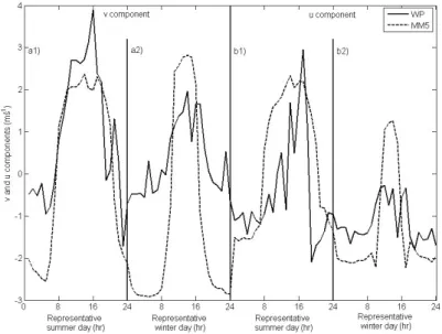
Fig. 9. Left panel: Diurnal cycle of v components, of near-surface winds, as measured by the wind profiler (solid line) and predicted by the MM5 numerical model (dashed line) for the representative summer (a1) and winter (a2) days. Right panel: Diurnal cycle of u components, of near-surface winds, as measured by the wind profiler (solid line) and predicted by MM5 (dashed line) for the representative summer (b1) and winter (b2) days.
– Bulk PBL scheme (Deardorff, 1972), based on bulk-aerodynamic parameterization.
– High-resolution Blackadar PBL (Zhang and Anthes, 1982) is used to forecast the vertical mixing of hori-zontal wind, potential temperature, mixing ratio, cloud water, cloud ice and graupel.
– Burk-Thomson PBL predicts turbulent kinetic energy for use in vertical mixing, based on the Mellor-Yamada formulas (Burk and Thompson, 1989).
– Eta PBL, based on the Mellor-Yamada scheme with lo-cal vertilo-cal mixing (Janji´c, 1990, 1994), is used for fore-casting the vertical mixing of horizontal wind, potential temperature and mixing ratio.
– Gayno-Seaman PBL, based on the Mellor-Yamada TKE prediction, focuses on saturated conditions (Ballard et al., 1991); it is distinguished from others by the use of liquid-water potential temperature as a conserved vari-able, allowing the PBL to operate more accurately in
1544 L. Bianco et al.: Thermally driven circulation in a region of complex topography
Fig. 10. Comparison between average wind intensity, of near-surface winds, observed by the radar wind profiler (red line) and predicted by MM5 (blue line).
41
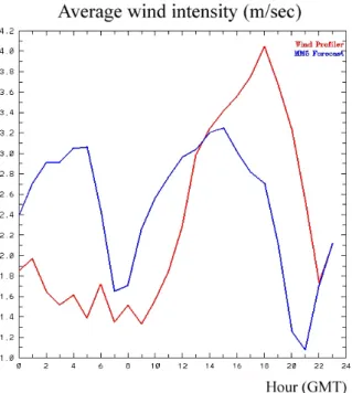
Fig. 10. Comparison between average wind intensity, of near-surface winds, observed by the radar wind profiler (red line) and predicted by MM5 (blue line).
saturated conditions (Ballard et al., 1991; Shafran et al. 2000).
– MRF PBL, based on a Troen-Mahrt representation for the countergradient term and K profile in the well-mixed PBL (Hong and Pan, 1996); the scheme is used to fore-cast the vertical mixing of horizontal wind, potential temperature, mixing ratio, cloud water, cloud ice and graupel.
– Blackadar’s non-local vertical mixing (Pleim and Chang, 1992).
The first scheme is suitable for a coarse vertical resolu-tion (Grell et al., 1995) and the last scheme works only when coupled with the Pleim-Xiu Land-Surface Model (Xiu and Plein 2000) and they were not selected for this study. We can group the other PBL parameterizations into two categories: local schemes (Burk-Thompson, Eta, and Gayno-Seaman) and non-local schemes (Blackadar and MRF). The Burk-Thompson scheme is not selected for this study because it is the only PBL option that does not call the SLAB scheme for surface temperature, as it has its own force-restore ground temperature prediction.
So, the PBL schemes used in this work are in detail: the High-Resolution Blackadar PBL scheme (Blackadar, 1976, 1979; Zhang and Anthes, 1982), which consists of a noctur-nal (stable) and a free convection (unstable) module of turbu-lent mixings; the Medium-Range Forecasts (MRF) scheme, also known as Hong and Pan PBL (Troen and Mahrt, 1986;
Hong and Pan, 1996), which is a non-local K scheme in which the countergradient transports of temperature and moisture under unstable conditions are added to the local gra-dient transports; the Gayno-Seaman scheme (Shafran et al., 2000), which is a Mellor Yamada (1974) 1.5-order closure model in which a prognostic equation for turbulent kinetic energy (TKE) is included; and the ETA PBL scheme also known as the Mellor-Yamada Janji´c scheme (Janji´c, 1990, 1994), which is a Mellor-Yamada level 2.5 scheme, or a vari-ant of 1.5-order closure model which includes a prognostic equation for TKE.
4 Results
4.1 Thermally-driven, near-surface winds
The study of the near-surface time evolution of the winds was divided into two subsets of results: summertime and winter-time, because, as it is reported in Figs. 3a–b, the analysis of surface winds carried out using long MM5 time series (years 1998–2005) showed that the average surface flow is quite dif-ferent for difdif-ferent seasons and it is dominated by southward winds during the winter season and eastward winds during summertime. For both summer and winter analysis, repre-sentative days are created to compare observed and simulated wind vectors. A “representative day” for radar wind profiler measurements is composed from the mean value of hourly wind vectors, over the clear sky days of the season under in-vestigation. In Figs. 3c–d we reproduce a typical case, one for summer and one for winter, showing the diurnal evolution of the circulation in the inner MM5 domain.
It is also interesting to know whether the model also cap-tured the day-to-day variability of the events. Table 2 shows the average and 6–12–24 hourly standard deviation for ob-served and predicted data. The model reasonably reproduces this variability index also within a short time scale (6 hours). For wintertime and summertime the averaged wind is over-estimated by the model (see also Fig. 10 and related discus-sion).
Figure 5 presents the summertime results for radar wind profiler observations, and Fig. 6 presents the numerical model prediction. Figures 7 and 8 are corresponding to Figs. 5 and 6, respectively, but they refer to the wintertime analysis. For all the figures, the diurnal evolution of the winds is presented in the upper panels; because wind vari-ability is an important parameter affecting the interpretation of computed vector resultant winds, their relative trend is in-troduced in the lower panels. Summer and wintertime analy-ses are discussed separately in the following paragraphs. 4.1.1 Summertime analysis
The mean, near-surface vector wind, computed starting from the radar wind profiler measured data, is presented in Fig. 5a and its persistence in Fig. 5b. Winds at this site are clearly
24h-Standard Deviation 2.29 1.76 0.56 0.66 2.36 1.91
the result of the mountain-valley interaction, and their di-rection is primarily northeasterly and southwesterly. Ther-mally driven winds are weak during the nighttime, when they drain from the mountain into the valley. Early in the morn-ing (08:00 –10:00 ), sunlight heats the surface and the winds start turning up-valley and increasing their strength. This is the morning transition period, during which the intensity of the wind starts to increase from values of 1 m s−1, found in the nighttime, reaching values of 2–3 m s−1. In the first pe-riod of the day winds are persistent, with lower values found in the transition period. The rotation continues to finally di-rect the flow from the valley toward the mountain during the warmest hours of the day (11:00 –18:00 ). The intensity of the wind reaches its maximum values (4–5 m s−1)early in
the afternoon, and the persistence shows very high values. At sunset, in accordance with the valley wind theory, the down-valley flow appears again (evening transition period), and completes the cycle that sees a complete clockwise turn during the whole daytime period. After sunrise, wind persis-tence has lower to moderate values, indicating that the resul-tant fair-weather day vector wind speed is smaller than the arithmetic average speed and that the wind direction is quite variable from day to day at this site, for these hours.
The same analyses, but relative to the numerical model predictions, are presented in Fig. 6, where the direction of the winds (Fig. 6a) is again primarily northeasterly and south-westerly. The morning transition period happens around 07:00 , when the wind persistence shows its minimum value (Fig. 6b). From 08:00 to 20:00 the flow is definitely directed up-slope and wind intensity is very uniform during the entire period, with values comparable to the measured ones. On the contrary, during the nighttime, the simulated winds are much larger than the ones obtained by the radar wind profiler. This is probably due to a possible overestimation of the modelled vertical momentum flux (Sang-mi Lee et al., 2005) and by an overestimation of mixed layer depth (Berg and Zhong, 2005) and in particular, an overestimation of mixing during a part of the day that results in excessive winds near the surface at night (Mass et al., 2002).
Both the experimental and numerical results complete the clockwise rotation with the evening transition, exhibited after the sunset, in agreement with the theory.
4.1.2 Wintertime analysis
During the wintertime (Figs. 7 and 8), the general behavior of the near-surface wind flow is again in accordance with the theory, and the direction of the winds turns clockwise with time in both the radar wind profiler data (Fig. 7a) and the nu-merical model predictions (Fig. 8a). Measured and predicted mean wind systems are in good agreement but a more gentle rotation of the simulated wind vector during the representa-tive day is evident, similarly to the summertime analysis.
For both the observational and predicted results, the main differences with respect to the summer analysis are found in the determination of the morning and evening transition periods, which, in this case, happens at about 10:00 and 17:00 , respectively. In this sense, during the wintertime, the up-slope flow is limited in time, as a result of the shorter period of exposure of the area to sunlight. Moreover, look-ing at Figs. 7b and 8b, the computed wind persistence re-veals smaller values compared with those found in the sum-mertime, when the thermally driven circulation is apparently much better defined from day to day at the site. Finally, the wind speed is bigger in the wintertime than in the summer-time.
Differences between observed down-valley and up-valley persistence values, both for the summertime and wintertime analysis, could be due to the strong influence of the solar radiation on this type of circulations. In this sense the up-valley flow is better defined compared to the down-up-valley one, implying bigger values of the observed persistence dur-ing daytime compared to those computed durdur-ing the night-time. Moreover, differences between observed and simulated persistence could be linked to the different time sampling of the two data sets. More specifically, the wind profiler’s time series are taken at about a 5-min interval and then averaged over a period of one hour. Quantitatively, diurnal cycles of the v and u components, of the near-surface wind observa-tion, are presented in Fig. 9. In the left panel we show the diurnal cycle of the v components, as measured by the wind profiler (solid line) and predicted by MM5 (dashed line), for the representative summer day (a1) and winter day (a2). In the right panel we show the same comparison but between the observed (solid line) and simulated (dashed line) u com-ponents for the representative summer day (b1) and winter
1546 L. Bianco et al.: Thermally driven circulation in a region of complex topography
Fig. 11. Time-height evolution of the wind vector during the representative day, as observed by the Wind Profiler (WP) (Fig. 11a), and as predicted by the MM5 using different PBL parameterizations: GAYNO (Fig. 11b), MRF (Fig. 11c), ETA (Fig. 11d), and BLAC (Fig. 11e).
42
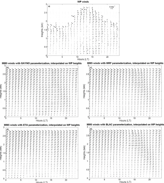
Fig. 11. Time-height evolution of the wind vector during the representative day, as observed by the wind profiler (WP) (Fig. 11a), and as predicted by the MM5, using different PBL parameterizations: GAYNO (Fig. 11b), MRF (Fig. 11c), ETA (Fig. 11d), and BLAC (Fig. 11e).
day (b2). Figure 9 is an encouraging result for the purpose of our analysis. It confirms the information revealed in Figs. 5– 8: the numerical model predictions, even if smoother than the experimental ones, are able to follow the temporal ten-dency in the wind vector clockwise rotation measured by the radar wind profiler.
In a statistical analysis performed on the entire data set (i.e. the entire year), the correlation coefficients between the wind components, of the near-surface wind observation, measured by the radar wind profiler and those predicted by the numer-ical model are 0.81 and 0.66, for v and u, respectively.
In Fig. 10, we show the comparison between the wind intensity measured by the wind profiler, averaged over the whole data set, and those predicted by MM5. The model re-produces well the average wind variation during the daytime while it significantly overestimates the average wind during the nighttime. This is in agreement with previous studies (see Zhang and Zheng, 2004) which found an underestimation of the strength of the surface wind speed during the daytime and an overestimation of it at night.
4.2 MM5 sensitivity to the PBL parameterization
The operational setting of the MM5 uses a Hong-Pan PBL parameterization scheme (MRF) suitable for high-resolution in PBL, but in this study we decided to proceed with the work
set of experimental data, but we were forced to choose a sub-set of 18 cases of fair-weather days. The subsub-set of cases was selected in the summer period, when the thermally driven cir-culation is well defined. Over this subset of cases the wind vector was averaged for every time of the day and for all the heights, to give a picture of a representative day for both wind profiler measurements and MM5 outputs. Figure 11 shows the time-height evolution of the wind vector during the repre-sentative day, as observed by the wind profiler (Fig. 11a), and as predicted by the MM5 using different PBL parameteriza-tion: GAYNO (Fig. 11b), MRF (Fig. 11c), ETA (Fig. 11d), and BLAC (Fig. 11e). Values of the MM5 wind predictions are interpolated on the wind profiler heights.
For all the different parameterization schemes (Figs. 11b–e) the mean wind flow is mainly southeastward and eastward. This behavior is similar to the observational one (Fig. 11a). The thermally driven rotation is present for the entire first height of the model outputs and it prop-agates through the first heights of the wind vector profile. Nighttime values of the predicted surface wind strength overestimate the observational ones during nighttime hours in all the schemes. The numerical simulation performed on the selected subset of data shows that the mean wind flow is slightly sensitive to the PBL parameterizations and this is coherent with the results obtained by other authors (e.g. Zhong and Fast, 2003). At a first sight, the GAYNO PBL scheme (Fig. 11b) seems to give an overestimation of the wind values compared to the wind profiler measurements (Fig. 11a) and to the other schemes, as well (Figs. 11c, d, and e). Very small differences are visible among the other schemes (MRF, ETA, and BLAC). To objectively test this sensitivity, Table 3 presents a statistical comparison between the MM5 predictions and wind profiler measurements, in terms of correlation coefficients for u and v components of the wind vector. Correlation coefficients introduced in Table 3 are computed on the subset of data, where we decided to focus the study of MM5 sensitivity on the PBL parameterization (i.e. the subset of 18 chosen cases). The computation of correlation coefficients has been performed on a total of 28×24 u and v measured and simulated components (where 28 is the number of wind profiler levels, and 24 the numbers of hours in the representative day). The comparison has been possible for the levels and the hours when wind profiler measurements were present.
For the cases under study the wind vector calculated by using the GAYNO PBL scheme is the one with the smaller agreement with the observations, while the simpler MRF
vcomponent 0.65 0.80 0.77 0.73
PBL scheme agrees better with the measurements. The val-ues of the correlation coefficients found in the statistical com-parison performed on the whole PBL are close to those found in the near-surface analysis. In this perspective the present analysis shows that the thermally driven flows are slightly influenced by model errors.
5 Summary and conclusions
In this study thermally driven circulation was investigated and MM5 predictions were validated in a site of complex topography, located in Central Italy (Assergi, L’Aquila), at 42.50◦N of latitude, 13.50◦E of longitude, and 981 m (ASL)
of altitude. The site is inland and placed at the southwest foothills of the Gran Sasso peak (2912 m ASL); it sees the regular slope of the mountain to its north–northeast direction and the valley to its south–southwest side. A whole year of data (22 May 2002–22 May 2003) was considered for the analysis. The observational data set consists of hourly wind data collected by a radar wind profiler located at the site. These data were used to test the 3-D MM5 model output. In the one-year data set, summer months of May, June, July, August, and September were extracted and analyzed sepa-rately to form the remaining period, in order to study the thermally driven circulation in the summertime and winter-time individually. For both summerwinter-time and winterwinter-time we investigated the diurnal evolutions of near-surface winds and computed vector averages to obtain hourly wind vectors for a representative day at the site. Furthermore, to better un-derstand the wind mechanism at the site, we tested the vari-ability of the wind vector through the determination of wind persistence, which is an indication of the steadiness of the wind over a continuous time period. To detect the thermally driven circulation, revealed in near-surface flows, we used only the measurements relative to the first height reached by the instrument and compared them with the numerical model predictions.
Thermally driven winds were observed during both sum-mertime and wintertime. Winds were generally down-slope and down-valley during the nighttime, and slope and up-valley during the daytime, as expected from the theory. Due to the slope of the valley, the thermally driven winds turn
1548 L. Bianco et al.: Thermally driven circulation in a region of complex topography clockwise during the representative day for both the
ana-lyzed subsets (summer and winter periods); the only dif-ference between them was found in the detection of morn-ing and evenmorn-ing transition periods. The up-slope flows were found to be more limited in time during the wintertime as a result of the area shorter period of exposure to sunlight. The thermally driven system was also revealed in the nu-merical model predictions, which also revealed the shorten-ing of the up-slope flow in the wintertime. The main dif-ference between experimental results and numerical predic-tions was found in the intensity of the wind vector relative to the averaged values over the whole data set. The MM5 tendency to underestimate the strength of the surface wind speed during the daytime, and overestimate it at night, com-pared to experimental data, has been observed before (Zhang and Zheng, 2004). Moreover, for both the two representative days, the numerical model appears to have an on/off switch to the up-valley/down-valley flow while the observed situ-ations are more confused; as discussed in the Introduction, this rapid up-valley/down-valley switch is probably due to the absence of a Land Surface Model. This leads to an un-realistic fast warming and cooling of the near-surface layers, resulting in a shorter transition phase with respect to the ob-served one. For all the analyses, wind persistence was high during the daytime for the radar wind profiler measurements, medium during the nighttime, and with lower values during the transition periods. The same variable computed for the predicted wind vectors showed lower values during the win-ter daytime and very low values in the transition periods, but very high values elsewhere. The analysis of the diurnal cycle of the v and u component, of near-surface winds, measured by the radar wind profiler and predicted by the MM5, con-firmed that the model simulation is able to follow the tempo-ral tendency in the wind vector clockwise rotation measured by the radar wind profiler. In a statistical analysis, values of the correlation coefficients between the v and u components measured by the radar wind profiler and those predicted by the numerical model over the entire year were found to be 0.81 and 0.66, respectively.
Because the thermally driven flows can have some depth and may be influenced by model errors, we extended our analysis to include the whole PBL. In this context we more-over explored the MM5 sensitivity to four different PBL pa-rameterizations (Gayno-Seaman, Medium-Range Forecast, ETA, and Blackadar) on a subset of 18 fair-weather days. For all of them we looked at the MM5 output for the whole PBL levels. The reason was to test how much the result was sensitive to the selected parameterization and to iden-tify the parameterization that works better. In a statistical comparison between the MM5 predictions and wind pro-filer measurements in terms of correlation coefficients for the u and v components (computed over the chosen subset of cases), we found that for the cases under study the wind vector calculated by using the GAYNO PBL scheme is the one with a smaller agreement with the observations, while
the simpler MRF PBL scheme is the one which agrees better with the measurements. According to the results of Song et al. (2003), the MRF PBL performs better among the tested PBL schemes. Of course, further case studies over different geographical regions are needed to test the capabilities of dif-ferent PBL schemes to realistically reproduce PBL features. Acknowledgements. The authors would like to thank R. Ferretti and her group of CETEMPS Center of Excellence for daily providing meteorological forecast; ARSSA (Regional Agency for Agriculture Service), in particular R. Zauri, for providing the solar radiation observations used in this work; and L. Ricciardulli for the many useful discussions. Moreover we wish to thank the two anonymous reviewers for their insightful comments.
Topical Editor F. D’Andrea thanks two referees for their help in evaluating this paper.
References
Atkinson, B. W.: Mesoscale atmospheric circulation, Academic Press, London 1981, 1981.
Ballard, S. P., Golding, B. W., and Smith, R. N. B.: Mesoscale model experimental forecasts of the haar of northeast Scotland, Mon. Wea. Rev., 119, 2107–2123, 1991.
Berg, L. K. and Zhong, S.: Sensitivity of MM5-simulated bound-ary layer characteristics to turbulence parameterizations, J. Appl. Meteor., 44, 1, 1467–1483, 2005.
Blackadar, A. K.: Modeling the nocturnal boundary layer, Third Symp. on Atmospheric Turbulence, Diffusion and Air Quality, Raleigh, NC, Amer. Meteor. Soc., 46–49, 1976.
Blackadar, A. K.: High resolution models of the planetary bound-ary layer: Advances in Environmental Science and Engineering, edited by: Pfafflin, J. and Ziegler, E., 1, Gordon and Breach, 50– 85, 1979.
Burk, S. D. and Thompson, W. T.: A vertically nested regional numerical prediction model with second-order closure physics, Mon. Wea. Rev., 117, 2305–2324, 1989.
Defant, F.: Local winds, Compendium of meteorology, edited by: Malone, T. F., Amer. Meteor. Soc., 655–672, 1951.
Deardorff, J. W.: Parameterization of the planetary boundary layer use in general circulation models, Mon. Wea. Rev., 100, 93–106, 1972.
Dudhia, J.: A nonhydrostatic version of the Penn State/NCAR mesoscale model: Validation test and simulation of an Atlantic cyclone and cold front, Mon. Wea. Rev., 121, 1493–1513, 1993. Green, R. J., Fred, U. P., and Norbert, W. P.: Things that go bump
in the night, Psych. Today, 46, 345–678, 1990.
Grell, G. A., Dudhia, J., and Stauffer, D. R.: A Description of the fifth generation Penn State/NCAR Mesoscale Model (MM5), NCAR Technical Note, NCAR/TN-398+STR, 121, 1994. Hawkes, H. B.: Mountain and valley winds with special reference to
the diurnal mountain winds of the Great Salt Lake region, Ph.D. dissertation, Ohio state University, 312, 1947.
Hong, S. H. and Pan, H. L.: Nonlocal boundary layer vertical dif-fusion in a medium-range forecast model, Mon. Wea. Rev., 124, 2322–2339, 1996.
Horel, J., Splitt, M., Dunn, L., Pechmann, J., White, B., Ciliberti, C., Lazarus, S., Slemmer, J., Zaff, D., and Burks, J.: MesoWest:
rameterization, J. Atmos. Sci., 47, 2784–2802, 1990.
Mass, C. F., Ovens, D., Westrick, K., and Colle, B. A.: Does in-creasing horizontal resolution produce more skilful forecasts?, Bull. Amer. Meteor. Soc., 83, 407–430, 2002.
Mellor, G. L. and Yamada, T.: A hierarchy of turbulence closure models for planetary boundary layers, J. Atmos. Sci., 31, 1791– 1806, 1974.
Panofsky, H. A. and Brier, G. W.: Some applications of statistics to meteorology, the Pennsylvania State University, 224, 1965. Paolucci, T., Bernardini, L., Ferretti, R., and Visconti, G.: MM5
real-time forecast of a catastrophic event on May, 5 1998, Il Nuovo Cimento, 12, 727–736, 1999.
Pielke, R. A.: Mesoscale meteorological modeling, 2nd Edition, Academic Press, San Diego, CA, 676, 2002.
Pleim, J. and Chang, J. S.: A non local closure model for vertical mixing in the convective boundary layer, Atmos. Environ., 26A, 965–981, 1992.
Sang-mi Lee, Giori, W., Princevac, M., and Fernando, H. J. S.: Implementation of a stable PBL turbulence parameterization for the mesoscale model MM5: nocturnal flow in complex terrain, Bound.-Layer Meteor., doi:10.1007/s10546-005-9018-4, 2005. Shafran, P. C., Seaman, N. L., and Gayno, G. A.: Evaluation of
nu-merical predictions of boundary layer structure during the Lake Michigan ozone study, J. Appl. Meteor., 39, 412–426, 2000. Song, Q., Hara, T., Cornillon, P., and Friehe, C. A.: A
Compari-son between observations and MM5 simulation of the marine at-mospheric boundary layer across a temperature front, J. Atmos. Ocean. Tech., 21, 170–178, 2003.
Stewart, J. Q., Whiteman, C. D., Steenburgh, W. J., and Bian, X.: A climatological study of thermally driven wind system of the U.S. Intermountain West, Bull. Amer. Meteor. Soc., 83, 699–708, 2002.
Winds), Gerlands Beitr. Geophys., 52, 408–449. English trans-lation by Whiteman, C. D., and Dreiseitl, E., 1984: Alpine me-teorology: Translation of classic contribution by Wagnar, A., Ekhart, E., and Defant F., PNL-5141 / ASCOT-84-3, Pacific Northwest Laboratory, Richland, WA, 121, 1938.
Whiteman, C. D. and Allwine, K. J.: Extraterrestrial solar radiation on inclined surfaces, Environ. Software, 1, 164–169, 1986. Whiteman, C. D.: Observations of thermally developed wind
sys-tems in mountainous terrain. Atmospheric processes over com-plex terrain, Meteor. Monogr., Amer. Meteor. Soc., 45, 5–42, 1990.
Whiteman, C. D., Bian, X., and Sutherland, J. L.: Wintertime sur-face wind patterns in the Colorado River valley, J. Appl. Meteor., 38, 1118–1130, 1999.
Xiu, A. and Pleim, J. E.: Development of a land surface model. Part I: Application in a mesoscale meteorology model, J. Appl. Meteor., 40, 192–209, 2000.
Zhang, D. L. and Anthes, R. A.: A high-resolution model of the planetary boundary layer – Sensitivity tests and comparisons with SESAME-79 data, J. Appl. Meteor., 21, 1594–1609, 1982. Zhang, D. L., Chang, H. R., Seaman, N. L., Warner, T. T., and
Fritsch, J. M.: A two-way interactive nesting procedure with variable terrain resolution, Mon. Wea. Rev., 114, 1330–1339, 1986.
Zhang, D. L. and Zheng, W. Z.: Diurnal cycles of surface winds and temperature as simulated by five boundary layer parameteri-zations, J. Appl. Meteor., 43, 157–169, 2004.
Zhong, S. and Fast, J.: An evaluation of the MM5, RAMS, and Meso-Eta models at subkilometer Resolution using VTMX Field Campaign Data in the Salt lake Valley, Mon. Wea. Rev., 131, 1301–1322, 2003.