HAL Id: hal-00317819
https://hal.archives-ouvertes.fr/hal-00317819
Submitted on 28 Jul 2005
HAL is a multi-disciplinary open access
archive for the deposit and dissemination of
sci-entific research documents, whether they are
pub-lished or not. The documents may come from
teaching and research institutions in France or
abroad, or from public or private research centers.
L’archive ouverte pluridisciplinaire HAL, est
destinée au dépôt et à la diffusion de documents
scientifiques de niveau recherche, publiés ou non,
émanant des établissements d’enseignement et de
recherche français ou étrangers, des laboratoires
publics ou privés.
observed with CHAMP
K. Schlegel, H. Lühr, J.-P. St.-Maurice, G. Crowley, C. Hackert
To cite this version:
K. Schlegel, H. Lühr, J.-P. St.-Maurice, G. Crowley, C. Hackert. Thermospheric density structures
over the polar regions observed with CHAMP. Annales Geophysicae, European Geosciences Union,
2005, 23 (5), pp.1659-1672. �hal-00317819�
SRef-ID: 1432-0576/ag/2005-23-1659 © European Geosciences Union 2005
Annales
Geophysicae
Thermospheric density structures over the polar regions observed
with CHAMP
K. Schlegel1, H. L ¨uhr2, J.-P. St.-Maurice3, G. Crowley4, and C. Hackert4
1Max-Planck-Institut f¨ur Sonnensystemforschung, Katlenburg-Lindau, Germany 2GeoForschungsZentrum Potsdam, Potsdam, Germany
3Institute for Space and Atmospheric Studies, University of Saskatchewan, Saskatoon, Canada 4Southwest Research Institute, San Antonio, TX, USA
Received: 15 November 2004 – Revised: 22 March 2005 – Accepted: 3 May 2005 – Published: 28 July 2005
Abstract. We report on the unexpected detection of consid-erable structure in high latitude thermospheric densities, as derived from an accelerometer onboard the CHAMP satel-lite. The width of the structures, which can either be maxima or minima, varies between a few hundred km and 2000 km. The amplitudes of these density extrema can reach 50% of ambient. Maxima cluster around 75◦(N and S), while min-ima are found closer to the poles. In a magnetic latitude– magnetic local time frame the maxima are found mainly around the cusp region. Overall, the observed structures somewhat resemble so-called density cells previously found in model calculations. However the models generate their cells around 140–300 km altitude and show little, if any rem-nant at 400 km or above. This has to be contrasted with the fact that the CHAMP observations were obtained near 430 km altitude. We have explored Joule heating as a possi-ble mechanism for the generation of the structures, at least in density enhancement regions, using Hall currents measured on CHAMP and simultaneous incoherent scatter measure-ments with EISCAT. However, the electric fields were usu-ally quite small during the period of observation, making the quest for an explanation for the structures all the more chal-lenging.
Keywords. Meteorology and atmospheric dynamics (Ther-mospheric dynamics) – Magnetospheric physics (Polar cap phenomena) – Atmospheric composition and structure (Pres-sure, density, and temperature)
1 Introduction
The CHAMP satellite was launched on 15 July 2000 in an almost circular orbit with an inclination of 87.25◦. The satel-lite does more than 15 orbits per day. During the campaign described here its altitude varied between 390 km at perigee and 440 km at apogee. Among other instruments, the satellite
Correspondence to: K. Schlegel
carries a very sensitive accelerometer, the data of which can be used to derive neutral densities. Details of the processing procedure have been reported elsewhere (Liu et. al., 2005) and will not be repeated here. We simply want to mention here the basic principles.
The density ρ has been derived here from the measured acceleration along the ram direction,
ax =1/2CDAρVt2 (1) where x indicates the ram direction, CDis the so-called drag coefficient, A is the effective area of the satellite in the ram direction, and Vt is the velocity of the satellite relative to the ambient air along the track. It should be noted that Vt=Vs+Vnx where Vs is the satellite orbit velocity (mean value 7.62 km/s) and Vnx is the neutral head or tail wind along the orbit.
Variations in the drag can be easily derived from Eq. (1) to yield the result
1ax/ax=1ρ/ρ +21V /V + 1CD/CD+1A/A
≈1ρ/ρ +21Vnx/Vt+1CD/CD. (2) Possible variations in the effective area may in principle re-sult from attitude changes of the satellite. Since the satel-lite is stabilised in attitude to fractions of a degree during its flight, we can neglected such changes. There are there-fore 3 factors that can be responsible for any observed vari-ations in the drag. The first one, which is the focus of the present paper, is a variation in the neutral mass density. The second possible cause for a change in the drag is neutral wind variations. However, while locally high neutral ve-locities exceeding 1 km/s have occasionally been reported in the high latitude thermosphere during disturbed conditions (Killeen et al., 1995), in our case Vnx probably does not ex-ceed 0.3 km/s, since the data was obtained during very quiet conditions. A value less than 0.3 km/s is also supported by neutral wind models such as HWM1993 and the first princi-ples model discussed below. With Vnx=0.3 and Vt=7.6 km/s, the second term in Eq. (2) would thus be smaller than 0.1 and
would introduce at most 10% changes in the drag (a more detailed calculation was provided by Schoendorf and Crow-ley, 1995). Our relative drag variations are generally consid-erably greater than 10%, and we have therefore simply ne-glected neutral wind effects below. This should nevertheless be kept in mind when we interpret the acceleration changes solely as neutral density changes in this paper. A third factor that also has nothing to do with density variations can influ-ence the drag in the ram direction, namely, as Eq. (2) illus-trates, changes in the drag coefficient itself. With the satellite not even close to being spherically symmetric, any change in attitude is liable to change the drag coefficient, possibly sig-nificantly. There are two strong arguments that changes in CDcannot explain our experimental results: First, a correla-tion test of the measured axdata with all three attitude angles performed for a number of cases was negative. Second, the time scale of attitude changes are large (several 10 min) com-pared to the observed short-time changes in ax(10–30 s), due to the large inertia of the satellite and the comparatively weak attitude control jets.
We are left to conclude that any relative change in the drag well in excess of 5% are probably caused by variations in the neutral atmospheric density. To take into account the changes in densities that were simply related to altitude variations, we have normalized the results such that the inferred densi-ties were all referred to a mean satellite height of 430 km. This reference was chosen because it represented the mean altitude at high latitudes (ϕ>60◦ and ϕ<−60◦). The ac-tual height in these regions acac-tually varied slowly (timescale
∼1 h) between 408 km and 440 km. We used a barometric law for the normalization, assuming the scale height to be 59 km which is deduced from the MSIS model for the pre-vailing conditions. It can easily be shown that uncertain-ties in Texof the order of 100–200 K would introduce errors less than 5% in our calculated densities. Again it should be remembered that the time scales of the observed accelera-tion changes interpreted as density structures are less than a minute.
Besides the accelerometer data, results from a highly ac-curate magnetometer were used in this study. By assuming a series of infinite line currents Hall currents can be derived from the magnetometer results (see Ritter et al., 2004, for details). We have used these Hall currents together with conductances obtained from ground based incoherent scat-ter measurements to estimate local electric fields and Joule heating rate in at least parts of the Northern Hemisphere.
The ground based data were obtained during a 7-day cam-paign, called SIRCUS (Satellite and Incoherent Scatter Radar
Cusp Studies, Watermann et al., 2005), from 16–22 February
2002. In this campaign three of the EISCAT radars were operating: the VHF radar located at Tromso and the two UHF radars located on Spitsbergen. Since the main aim of this campaign was the study of cusp phenomena, the radars operated every day between 08:00 and 13:00 UT, i.e. dur-ing the time interval when the cusp is usually located above Spitsbergen. The days of the campaign were chosen so that CHAMP was passing through this area several times a day
in the pre-noon sector. We should emphasize that the days of the SIRCUS campaign were relatively quiet from the geo-magnetic activity point of view. The daily Ap was 4.8, 11.6, 10.6, 5.9, 7.8, 7.8, 7.8 during this week.
A small subset of the data discussed in the present work has already been presented elsewhere (L¨uhr et al., 2004), pointing out density enhancements in the northern cusp re-gion. Here we extend that study by examining a larger data set covering an entire week for both hemispheres, and by examining both density maxima and minima. Thermo-spheric neutral density structures have been observed before, although not with the high resolution of the CHAMP data: In OGO6 density data (Taeusch and Hinton, 1975; Taeusch 1977) in ESRO4 densities (Pr¨olss, 1981; Pr¨olss et al., 1988; Caspers and Pr¨olss, 1999), and onboard the S85-1 and SETA satellites (Crowley et al., 1989a, b, 1995, 1996; and Schoen-dorf et al., 1996a). Except for the OGO6 data gathered at an average altitude of 450 km all the previous measurements have been performed at a substantially lower altitude than the CHAMP data. The first predictions by a model, the Thermo-spheric General Circulation Model were reported by Crowley et al. (1989a, b).
Our main results are presented in the next section. This is followed by a comparison with model calculations in Sect. 3 where we find that, for some reason, the model is unable to reproduce the observations at the altitudes of interest. In Sect. 4, we also attempt to link the density enhancements with Joule heating, only to conclude that there were no obvi-ous Joule heating events that could be seen in our particular data set.
2 Polar density structures
We start our presentation with an example, in Fig. 1, of results obtained for a satellite trajectory over the northern polar region in a geographic latitude–local time frame. In this example, the satellite crosses the +60◦-latitude circle at 09:33 LT on the day side and at 20:54 LT on the night side. In the lower panel of the figure we have plotted as a solid line the density derived from the drag data along the satellite path. The dashed line shows an average undisturbed density ρav which has been derived for the whole orbit with a smoothing technique described below. In this particular example, den-sity enhancements are evident on both sides of the pole (up to 50% at about 80◦in the morning) with a weak density re-duction near the pole (more examples are presented in Figs. 3 and 9).
We have systematically studied the appearance and the properties of the density structures, for the seven days of the SIRCUS campaign. Each significant maximum or minimum was fitted to a Gaussian viz
f (s) = aexp −(s − s0)
2
b2 ln(2)
!
, (3)
where s is a distance along the track which was derived by multiplying the flight time with the average satellite velocity
Fig. 1. Example of a CHAMP trajectory over the northern polar re-gion in a geographic latitude–local time frame. The lower panel shows the density along this trajectory as obtained from the ac-celerometer data. The dotted line indicates an average undisturbed density ρav.
of 7.62 km/s. The accelerometer data were averaged over 10 s, corresponding to 1s=76.2 km. The parameter a is the amplitude of the density structure (“density amplitude” in the following). It will be expressed here either as an absolute density amplitude, obtained by subtracting ρavfrom the ac-tual density ρ, or as the magnitude of the relative density amplitude (ρ−ρav)/ρav. The parameter 2b is called width throughout the paper, and is expressed in km. Please note that we defined the width at the point where the exponen-tial function had decreased to a/2 which explains the factor ln(2). The center of the Gaussian, s0, is expressed in terms
of geomagnetic latitude and magnetic local time.
Great care was taken to characterize ρav, the undisturbed density along the track. We approximated it by successively applying a third order polynomial twice for a whole orbit. We also tried polynomials of higher orders and other smoothing procedures, but the results for the density amplitudes a all agreed within a few per cent. We therefore accepted 4–6%
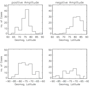
Fig. 2. Distribution of the amplitude of the density maxima (right hand part) and of the minima (left hand part) for the Northern (upper panel) and Southern (lower panel) Hemisphere.
as a workable uncertainty for a (see below).
It should be noted that CHAMP’s orbital plane moves through local time at a rate of 1 h per 11 days. This means that the local time when crossing the 60◦latitude circle as given in Fig. 1 changes by only a few minutes during one day. Due to the separation between the geographic and magnetic poles, the CHAMP tracks cover a range of about 3 h in magnetic local time (MLT) across the poles, which does not change very much during the 7-day campaign (see Figs. 6a, b).
The distributions of the absolute density amplitudes are displayed in Fig. 2 for the Northern (upper panel) and the Southern Hemisphere (lower panel). We used only density amplitudes in excess of alimit=0.5×10⁻¹²kg/m3 in the following (corresponding to relative amplitudes
(ρ−ρav)/ρav=4-6%). We adopted this limit because uncer-tainties associated with the method used to obtain ρav, as well as those associated with our neglect of neutral wind ef-fects make smaller amplitudes quite uncertain in terms of an actual density perturbation.
For the Northern Hemisphere the density amplitude dis-tribution is remarkably symmetric, i.e. the number of sity maxima (112) equals roughly the number of den-sity minima (115). The average of the density max-ima is 1.37×10⁻¹²kg/m3, and the average of the min-ima is –1.3×10⁻¹²kg/m3. Since the mean density over the Northern Hemisphere (geomagnetic latitude >60◦) is 7.6×10⁻¹²kg/m3, this means that the absolute average density amplitudes correspond to relative average density
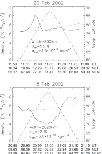
20.85 20.90 20.95 21.00 21.05 21.10 21.15 UT 08.63 08.36 07.62 02.58 22.34 21.65 21.39 MLT 52.59 64.94 77.17 85.23 76.28 64.22 51.25 MLAT 11.50 11.55 11.60 11.65 11.70 11.75 11.80 UT 10.34 10.86 12.29 16.77 19.68 20.53 20.87 MLT 55.17 67.48 77.91 81.47 73.36 62.03 50.00 MLAT
Fig. 3. Two examples of large-amplitude maxima and minima (solid line). The dotted line is the average undisturbed density ρav, the
dash-dotted line indicates the geographic latitude. The legend gives the absolute and relative density amplitude and the width.
amplitudes of 17.6% and –17.3%, respectively. The am-plitude distribution for the Southern Hemisphere is, by con-trast, rather asymmetric. We found 132 density maxima and only 72 density minima. The average amplitude of the max-ima is 1.48×10⁻¹²kg/m3, and the average of the minima – 1.08×10⁻¹²kg/m3(corresponding to relative density ampli-tudes of 15.4% and –11.5%). The asymmetry may be due to a bias in the mean undisturbed density ρav, defined above, i.e.
ρavmay be systematically too low over the Southern Hemi-sphere. However, we did not treat the Southern Hemisphere differently in this respect, as the mean undisturbed density
ρavwas always calculated for the whole orbit. A more proba-ble explanation for the asymmetry stems from the orbital ge-ometry of CHAMP during our campaign: As will be shown in what follows, the minima are mostly located quite close to the magnetic pole in the Northern Hemisphere. For the Southern Hemisphere, fewer CHAMP orbits get close to the magnetic south pole (see Fig. 6b), because of the larger offset between the geographic and magnetic poles in the Southern
Hemisphere, and therefore fewer minima are likely to be en-countered if minima cluster near the pole
Two of the extreme cases of maxima and minima are de-picted in Fig. 3. The upper plot shows a large, but narrow maximum with a density amplitude of a=3.5×10⁻¹²kg/m3 (a/ρav=53%) and a width of 800 km. The lower part depicts the broadest structure that was found during the seven days of the campaign, a deep and broad minimum with an am-plitude of a=3.0×10⁻¹²kg/m3(a/ρav=42%) and a width of 2620 km. In this latter case, the minimum is adjacent to a maximum (after 21:08 UT).
The distribution of density structures as a function of geo-magnetic latitude is shown in Fig. 4. In the Northern Hemi-sphere (upper row) the occurrence in density maxima reaches a distinct peak at 75◦–78◦, with the average at 75.4◦. The distribution in the minima is not as sharp, though the av-erage latitude, 81.5◦, is distinctly higher than for the max-ima. Thus, density minima are found at latitudes closer to the magnetic north pole than enhancements. In the Southern Hemisphere (lower row) the maxima occur mainly between –69◦and –81◦, while the average latitude is –78.6◦. The min-ima are even more broadly distributed than in the Northern Hemisphere, with a latitudinal range covering between –66◦ and –81◦and an average latitude of –75.3◦. Thus, by con-trast with the Northern Hemisphere, there is no significant difference between the average location of the maxima and the minima. For the sake of completeness we also prepared similar plots versus geographic latitude (not shown). They cover in principle about the same range in degrees, although their distribution is somewhat broader and not as distinct as when the plots are made as a function of geomagnetic lati-tude. We conclude that the description of the location of the density structures is more appropriate in terms of geomag-netic rather than geographic latitude. A similar conclusion was reached by Taeusch and Hinton (1975) and, purely from modelling results, by Crowley et al. (1995, 1996).
Figure 5 displays the distribution of the widths (2b) of the density structures. The figure shows that density en-hancements are generally narrower than 1000 km in both the Northern and Southern Hemispheres, with average widths of 790 km and 860 km, respectively. The density minima on the other hand are broader. They are, in addition, more broadly distributed. Their average width is 1070 km for the northern and 970 km for the Southern Hemisphere. This being stated, it has to be underscored that the “width” reported here only corresponds to the diameter of a structure when the satellite moves exactly through the center of a structure. In that sense, the widths reported here may be smaller than the actual struc-ture sizes.
In Fig. 6a we summarize the local and temporal behaviour of the density structures observed over the Northern Hemi-sphere (magnetic latitude >60◦) during the SIRCUS cam-paign. The coloured tracks display the relative density
(ρ−ρav)/ρav for each 10-s data point (i.e. not only for the Gaussian-fitted extrema). The pattern which emerges is the following: strong density maxima generally occur around 75◦magnetic latitude (c.f. also Fig. 4) between about 10:00
Fig. 4. Distribution of the maxima (left column) and minima (right column) as a function of geomagnetic latitude for the Northern (up-per row) and Southern (lower row) Hemisphere.
and 11:00 MLT on the day side. This turns out to corre-spond to the cusp region. Indeed, similar structures have al-ready been reported around the cusp by L¨uhr et al. (2004). On several days strong maxima can also be found some-what earlier, between 08:00 and 09:00 MLT. Apart from the cusp area, density maxima can also be seen between 21:00 and 22:00 MLT on the night side at lower magnetic lati-tudes (60◦–72◦). By contrast, density minima are found to be closer to the magnetic north pole, i.e. above 75◦MLAT, on the day as well as on the night side, sometimes even stretch-ing over the polar regions.
The corresponding summary for the Southern Hemisphere is displayed in Fig. 6b. Clearly, because of the larger off-set between magnetic and geographic poles in that case, the CHAMP tracks cover a wider range of MLT than for the Northern Hemisphere. This leads to the hemispheric dif-ference in the distribution discussed above. Nevertheless, strong maxima occur frequently at MLAT≈70–80◦between 10:00 and 11:00 MLT, i.e. over the southern cusp. In addi-tion we have strong maxima below 75◦MLAT in the early morning between 02:00 and 04:00 MLT. A clustering of minima seems to occur in the morning between 04:00 and 07:00 MLT.
A summary for the whole week is displayed in Fig. 7. Here we divided the two hemispheres into 30 MLAT and 72 MLT bins (i.e. each bin is 1◦ broad and 20 min in an-gular direction) and computed an average relative density
(ρ−ρav)/ρav from all orbits from 16 February 00:00 UT to 22 February 24:00 UT for each bin. The coloured areas correspond to the MLAT–MLT region covered by CHAMP during the 7-day campaign. There are generally one or more data points in each bin, except for those that are left white.
Fig. 5. Same as Fig. 4 but as a function of the width of the max-ima/minima.
Since CHAMP moves very fast in MLT over the pole, not every bin contains a data point close to the poles, particu-larly for the Southern Hemisphere where there is much more space between individual tracks (Fig. 6b). The white circles around the poles indicate the MLT range that is never reached by CHAMP. These summary plots offer a clear and succinct summary of the results discussed so far. That is to say: for the Northern Hemisphere (top), higher-than-average densi-ties occur mostly in the cusp region around 75◦MLAT at 10:00–11:00 MLT, while lower-than-average densities occur close to magnetic pole mostly at MLAT>75◦in the ing sector. Elevated densities can also be seen in the morn-ing at 08:00–09:00 MLT and weakly in the evenmorn-ing around 21:00 MLT at auroral latitudes, MLAT<72◦. Over the South-ern Hemisphere (bottom) we again have elevated densities in the cusp region, although we also can see other instances of enhancements scattered over the morning sector. Minima oc-cur at various locations but do seem to cluster in the high lat-itude morning sector, just as they did in the Northern Hemi-sphere. Note that we assume the cusp remaining at the same position during the whole 7-days period, due to the quiet con-ditions.
Finally, we also looked for a correlation between the den-sity amplitude and the solar zenith angle, in order to check if solar heating affects the density structures. No correlation was found, although we also have to state that, during our campaign, the solar zenith angles were quite high and cov-ered only a limited range between 80◦and 120◦in the north, and between 60◦–100◦in the south. Corresponding results for summer times and thus smaller zenith angles might yield different results.
11 07 23 MLT MLAT=60 MLAT=70 MLAT=80 MLT 22 19 20 21 09 10 08 11 07 23 MLAT=60 MLAT=70 MLAT=80 22 19 20 21 09 10 08 11 07 23 MLAT=60 MLAT=70 MLAT=80 22 19 20 21 09 10 08 0.25 0 -0.25 0.125 -0.125 16 Feb 2002 NH 17 Feb 2002 NH 18 Feb 2002 NH 11 07 23 MLT MLAT=60 MLAT=70 MLAT=80 MLT 22 19 20 21 09 10 08 11 07 23 MLAT=60 MLAT=70 MLAT=80 22 19 20 21 09 10 08 11 07 23 MLAT=60 MLAT=70 MLAT=80 22 19 20 21 09 10 08 19 Feb 2002 NH 20 Feb 2002 NH 21 Feb 2002 NH (a) 11 07 23 MLT MLAT=60 MLAT=70 MLAT=80 MLT 22 19 20 21 09 10 08 11 07 23 MLAT=60 MLAT=70 MLAT=80 22 19 20 21 09 10 08 11 07 23 MLAT=60 MLAT=70 MLAT=80 22 19 20 21 09 10 08 0.25 0 -0.25 0.125 -0.125 16 Feb 2002 SH 17 Feb 2002 SH 18 Feb 2002 SH 11 07 23 MLT MLAT=60 MLAT=70 MLAT=80 MLT 22 19 20 21 09 10 08 11 07 23 MLAT=60 MLAT=70 MLAT=80 22 19 20 21 09 10 08 11 07 23 MLAT=60 MLAT=70 MLAT=80 22 19 20 21 09 10 08 19 Feb 2002 SH 20 Feb 2002 SH 21 Feb 2002 SH (b)
Fig. 6. (a) The relative density along the CHAMP trajectories in a magnetic latitude–magnetic local time frame for the days 16 to 21 Febru-ary 2002, Northern Hemisphere. The density along the tracks is colour coded according to the scale in the middle. (b) Same as Fig. 6a but for the Southern Hemisphere.
3 Comparison of CHAMP and TIMEGCM results
Thermospheric General Circulation Models (TGCMs) were developed by the National Center for Atmospheric Research (NCAR) beginning in the early ‘80s to study the global tem-perature, circulation, and chemical structure of the thermo-sphere and its response to solar and auroral activity. A 3-D coupled thermosphere-ionosphere general circulation model (TI-GCM) was developed by Roble et al. (1988), and extended to include self-consistent electrodynamic interac-tions (TIE-GCM) between the ionosphere and thermosphere (Richmond et al., 1992). The model now extends down to 30 km, to include the mesosphere and upper stratosphere and is known as TIMEGCM (Roble and Ridley, 1994). It predicts winds, temperatures, major and minor composition, electron densities and electrodynamic quantities globally from 30 km to about 600 km altitude. In this paper, we present simula-tions using the TIMEGCM for comparison with the CHAMP data.
Crowley et al. (1989a, b) discovered the organized den-sity (and pressure and composition) cell structure in the neu-tral thermosphere at high latitudes using simulations from the TGCM. The morphology of the cells predicted by the TIMEGCM is substantially the same as from the TGCM and TIGCM. The number, location and amplitude of the density cells depend on magnetic activity level, and altitude. The morphology of the density cells for equinox solar minimum conditions was presented by Crowley et al. (1996) and for so-lar maximum conditions by Schoendorf et al. (1996a), using the TIGCM. The cells are also predicted by other global ther-mosphere models (e.g. Fuller-Rowell et al., 1999). The pre-ceding work focused on altitudes below about 250 km, and no effort has previously been made to observe the cells at altitudes above 400 km, where CHAMP makes its measure-ments.
Figure 8 summarizes the results from the present TIMEGCM simulation for 21 February 2002. It shows four polar plots of the neutral density in a geographic latitude– local time frame for the altitudes 450 and 200 km (rows) and for the Northern and the Southern Hemisphere (columns) at two different UT times. In the upper row we also plotted the trajectory of the CHAMP satellite. Recall that CHAMP passes from morning to evening over the Northern and from evening to morning over the Southern Hemisphere.
The density structures predicted at 200 km (lower panels) are typical of those discussed in earlier papers (e.g. Crowley et al., 1996). For magnetically quiet and moderate condi-tions, the density minima produced by the model are gener-ally well defined, and are almost circular in shape. There is also always only one minimum, with an average den-sity decrease of about 14% of the average denden-sity poleward of 60◦/–60◦ latitude. The width of this minimum is typ-ically about 1500 km and it never appears equatorward of 60◦/–60◦ latitude. In the Northern Hemisphere the mini-mum is confined to the sector 05:00 LT–10:00 LT during the whole day (travelling from 08:00 LT at 00:00 UT, to 05:00 LT at 08:00 UT, to 10:00 LT at 20:00 UT and back).
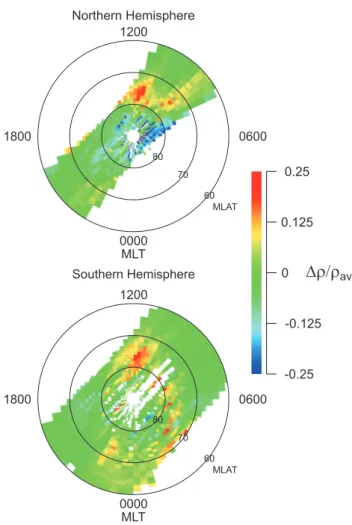
Average Neutral Density Enhancements and Reductions 16.02.2002 - 22.02.2002 0600 0000 MLT 1800 80 70 60 MLAT 1200 Southern Hemisphere 0.25 0 -0.25 0.125 -0.125 0600 0000 MLT 1800 80 70 60 MLAT 1200 Northern Hemisphere
Fig. 7. Average of the CHAMP derived relative densities for the whole 7-day interval of our campaign in a magnetic latitude– magnetic local time frame for the Northern (top) and Southern (bot-tom) Hemisphere. The average densities are calculated in bins of 1◦in MLAT and 20 min in MLT. The white areas are not covered by the satellite during the 7 days.
In the Southern Hemisphere the minimum circles around the pole during the day (from about 09:00 LT at 00:00 UT, to 23:00 LT at 11:00 UT, to 06:00 LT at 21:00 UT), because of the large offset of the geographic and magnetic poles. These apparent motions of the cells in geographic coordinates were discussed by Crowley et al. (1996).
The model-produced density maxima around 200 km are not as well isolated as the minimum. They spread out more, forming either one elongated enhancement opposite to the minimum, or two separated maxima. The average enhance-ment in Fig. 8 is about 9%, implying that the amplitude of the maxima, at least for the relatively quiet period under con-sideration, is significantly smaller than the amplitude of the mimima. At some UT times (not shown) the model-deduced maxima extend equatorward of 60◦/–60◦ latitude. In the Northern Hemisphere the maxima are confined to the sector
Fig. 8. Results from the TGCM model for the 21 February 2002. The upper row shows the density at 450 km altitude over the Northern (right) and the Southern (left) Hemisphere, the CHAMP trajectory is indicated with crosses. The lower row shows the density at 200 km altitude for both hemispheres, clearly structured in “cells”. Perimeter latitudes are 52.5◦N and 52.5◦S.
15:00 LT–02:00 LT, while in the Southern Hemisphere they circle the pole during the day, just as the minimum does.
The upper panels of Fig. 8 depict the model predictions for 450 km, near the height of the CHAMP satellite. Un-fortunately (but interestingly), the thermosphere produced by the TIMEGCM at 450 km is completely devoid of any of the structures described for lower altitudes and those ob-served by CHAMP around 430 km. The same is true for the TIMEGCM at 400 km altitude (not shown here). This re-duction in the amplitude of the modelled structures above 300 km was described by Schoendorf et al. (1996a), and the CHAMP data represent the first opportunity to test the pre-diction. While the failure of the model to reproduce the ob-servations is puzzling, we have nevertheless checked if the
structures observed by CHAMP were in qualitative agree-ment with the lower altitude cells identified by TIMEGCM. Although a comparison of results from very different height levels is problematic, Schoendorf et al. (1996a) have pre-dicted that above about 170 km, the MLT/latitude locations of the cells does not change significantly with altitude. We therefore compared the CHAMP results at 400 km altitude with the structures predicted by TIMEGCM for 200 and 300 km altitudes.
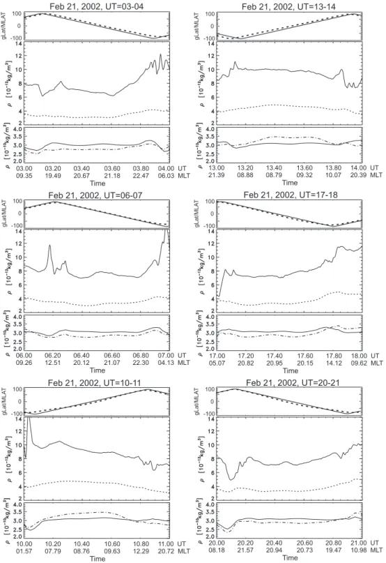
For a detailed comparison of the measured and the modelled densities we plotted the density along the CHAMP trajectory during six 1-h UT intervals (Fig. 9). We selected intervals during which CHAMP crossed the hemispheres close the north pole as well as close to the south pole (but
-100 0 100 gLat/MLA T 13.00 13.20 13.40 13.60 13.80 14.00 UT 21.39 08.88 08.79 09.32 10.07 20.39 MLT Time Feb 21, 2002, UT=13-14 -100 0 100 gLat/MLA T 17.00 17.20 17.40 17.60 17.80 18.00 UT 05.07 20.82 20.95 20.15 14.12 09.62 MLT Time Feb 21, 2002, UT=17-18 -100 0 100 gLat/MLA T 20.00 20.20 20.40 20.60 20.80 21.00 UT 08.18 21.57 20.94 20.73 19.47 10.98 MLT Time Feb 21, 2002, UT=20-21 -100 0 100 gLat/MLA T 10.00 10.20 10.40 10.60 10.80 11.00 UT 01.57 07.79 08.76 09.63 12.29 20.72 MLT Time Feb 21, 2002, UT=10-11 -100 0 100 gLat/MLA T 03.00 03.20 03.40 03.60 03.80 04.00 UT 09.35 19.49 20.67 21.18 22.47 06.03 MLT Time Feb 21, 2002, UT=03-04 06.00 06.20 06.40 06.60 06.80 07.00 UT 09.26 12.51 20.12 21.07 22.30 04.13 MLT Time -100 0 100 gLat/MLA T Feb 21, 2002, UT=06-07
Fig. 9. Comparison between CHAMP and TGCM results for six 1-h intervals on 21 February 2002, upper panels: satellite orbit as a function of time and geographic (solid) and magnetic (dashed) latitude, middle panels: CHAMP-derived densities (solid) and TGCM densities at 430 km altitude (mean satellite height) (dashed), lower panels: TGCM densities at 200 km altitude (solid) and 300 km altitude (dash-dotted). The values at 300 km have been multiplied by 10 in order to fit into the same density scale.
the results discussed below apply to all 24 intervals). The upper panel indicates the geographic latitude of the orbit. The middle panel shows the measured densities (solid line) normalized to an altitude of 430 km together with the model densities at this height. The observed densities are greater
than those obtained by the model by a factor of 2 on average, with sometimes considerably larger differences. This seems like an unexpectedly large discrepancy, but is not the focus of the work described here.
In the lower panel we plotted the model densities along the same path but at 200 km altitude (solid line) and 300 km altitude (dash-dotted line, multiplied by a factor of 10 to per-mit plotting on same scale as 200 km results). While there is no agreement between the model and data at 450 km, the following details emerge from the lower panels of the figure: some of the structures observed by CHAMP appear to have corresponding structures predicted by the model at 200 and 300 km. For example at UT=3.85, 6.27, 17.08, 17.85 (with the 300-km density), 20.10, 20.95. However, sometimes the measured and the modelled structures are shifted by several 100 km (remember that the satellite travels with 7.6 km/s) e.g. at UT=3.1–3.2. Quite often they are almost anti corre-lated e.g. at UT=3.96, 6.18, 6.98, 10.04, 10.90 13.12, 13.82. In this respect it should be noted however, that also the mod-elled structures at 200 and 300 km are not always in phase, e.g. at UT= 4.0, 10.9, 13.1, 13.95, 17.8. Only two qualita-tive agreements remain: (1) the CHAMP satellite sees these density structures only at high latitudes, like the model pre-dictions; (2) both the data and the model indicate that the density minimum is closer to the pole than the density max-ima.
There are other noticeable differences of a different kind between the CHAMP data and the model predictions for 200 and 300 km. Most notable is the fact that the clustering of density maxima in the cusp region observed by CHAMP (see Fig. 7) cannot be found in the TIMEGCM simulation results. In addition, the measured structures are smaller in scale and often show multiple extrema whereas the modelled structures are wider and form generally only one maximum or minimum. The data from the S85-1 and SETA satellites showed similar effects (Crowley et al., 1996; Schoendorf et al., 1996a). Another significant difference is the amplitude of the structures; the modelled densities exhibit relative changes of 9–14% at 200 km and about the same at 300 km, whereas the measured structure amplitudes even at 430 km are con-siderably larger, sometimes exceeding 50% (c.f. Sect. 2).
It remains the most obvious result of the comparison, that TIMEGCM does not produce structures above 350–400 km altitude where CHAMP observes them. This is difficult to explain, since according to the conservation of energy ampli-tudes of extrema should increase with altitude. The mech-anisms producing the density cells are not fully understood (Schoendorf et al., 1996b), but it is difficult to imagine that the mechanisms producing the density cells at 300 km are not present at 450 km. The discrepancy may be due to imper-fect upper boundary conditions in the model. On the other hand it is clear that all diffusive scales become very large above 250 km, so that particle diffusion may wipe out den-sity structures. Another explanation may be that the observed structures are caused by waves that are not properly included in the model. They may be the agent which counteracts the overwhelming influence of diffusion at high altitudes.
Regarding the much smaller scales of the structures which CHAMP observes, it is clear that the model cannot resolve them, since its resolution is limited to 5◦in latitude and lon-gitude (about 500 km). The observed multiple structures may
be waves, and in addition, the variable high latitude forcing encountered in the real atmosphere may set up variable re-sponses, whereas the high latitude forcing in the model is relatively smooth.
4 Possible connection to Joule heating
Inasmuch as the density enhancements seen by CHAMP were due to a vertical motion of the atmosphere, one would be tempted to look for a heating rate that could be responsible for these enhancements. The most obvious heating sources for the high latitude thermosphere are: solar EUV radiation, particle precipitation, Joule heating, and, possibly, dissipa-tion of atmospheric gravity waves (AGW) propagating from sources in the lower atmosphere. The first mechanism can be assumed to be well described by the TIMEGCM model, given the predictability of the process and the mature state of the model. The second process, particle precipitation, is less predictable and has taken a back seat to Joule heating in recent years, given that many studies have inferred that the Joule heating rate should dominate. The final mechanism, upward propagation of waves generated in the lower atmo-sphere, is the hardest to investigate: one has to decide where the waves are generated, and by what process. It is normally assumed that AGW’s would have dissipated by the time they reach the upper thermosphere, owing to the large diffusion coefficients.
Nonetheless, having made a comparison with TIMEGCM, we are led to conclude from Sect. 3 that neither EUV radia-tion nor large scale global processes are responsible for the structures seen by CHAMP. However, the SIRCUS campaign was planned in such a way that it could provide some infor-mation about Joule heating. In particular, CHAMP itself is able to produce good estimates of Hall currents through its magnetometers, and the ground-based data from three EIS-CAT radars were available to provide estimates on conduc-tance and electric fields. The radars also measured the ion temperature, which gives a handle on frictional heating rates and therefore on Joule heating rates in the area.
The (height-integrated) Pedersen current can be expressed in terms of conductance 6P, electric field E, and neutral wind Vnas
JP =6P(E + Vn×B) or
JP =6P|(E + Vn×B)| , (4) since we are dealing only with the magnitudes in the follow-ing discussion. If we separate the current in an E- and an F-region part, the Joule heating is then
Q = 6PE (E + V E n ×B) 2 +6PF (E + V F n ×B) 2 . (5) The Hall current measured onboard CHAMP is
JH =6H (E + V E n ×B) . (6)
We use only the E-region part here, since the Hall currents are dominated by contributions from this region. This means
0600 0000 MLT 1800 80 70 60 MLAT 1200
Average Hall Current Magnitude 16. - 22.02.02 Northern Hemisphere
0.15
0.10
0.05
0
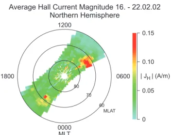
Fig. 10. Hall current magnitude averaged for all orbits of the seven days of our campaign in a magnetic latitude–magnetic local time frame.
that the Hall conductivity is negligible in the F-region. Com-bining Eqs. (5) and (6) we have
Q = 6 E PJ 2 H 62H +6PF (E + V F n ×B) 2 . (7)
Whereas the neutral wind in the E-region is usually quite small during quiet conditions, in the F-region the wind term may actually dominate over the electric field term. Unfortu-nately we have no information about the neutral wind during our measuring interval.
We had all the data necessary to evaluate the Hall current and both E- and F-region conductances, and could check whether the Joule heating rate was large enough to matter. The derivation of the Hall currents from the CHAMP mag-netic field measurements has been described in detail by Rit-ter et al. (2004) and verified with the help of the IMAGE ground-based magnetometer array. As a result we have ac-cepted the derived currents as reliable estimates. Also note that the following comparison was only performed for the Northern Hemisphere due to the lack of ground-based data for the other hemisphere.
We first plotted, in Fig. 10, |JH|in a magnetic latitude– magnetic local time frame averaged over all orbits of the seven days of our campaign. Two areas of maximal Hall currents can be seen: one in the morning sector around MLT≈08:00 at 69◦>MLAT>75◦and another in the evening around 21:30 MLT at 70◦<MLAT<74◦. It is unfortunate that the data don’t cover a broader local time range, but these seem to be parts of the well-known areas of the westward and the eastward electrojet in the auroral zone. It should be noted, furthermore, that even the observed average peak cur-rent densities of ≈0.17 A/m are quite small. This is consis-tent with the quiet conditions during which the observations were taken. During magnetic storms JH can easily exceed several A/m (e.g. Ritter et al., 2004). The fact that we have
quiet conditions here can also be seen in the contracted auro-ral oval: during disturbed conditions the electrojet would be located much further equatorward.
Figure 10 can be compared with Fig. 7, which showed the CHAMP relative density enhancements in the same for-mat. It is quite obvious that the MLAT–MLT range where the density maxima occur does not really agree with the MLAT– MLT range of the maximal Hall currents. Whereas the max-imal currents correspond reasonably well to the enhanced densities between 08:00–09:00 MLT and to the weaker en-hanced ones around 21:00–22:00 MLT, no current enhance-ments are found in the 10:00–11:00 MLT sector, where we see strongly elevated densities. From this result we may in-fer that these latter density enhancements are probably not caused by Joule heating due to the large-scale Pedersen cur-rents flowing perpendicular to the magnetic field, at least not in the E-region. A connection to the strong and fast varying local field-aligned currents observed by CHAMP and other satellites in the cusp area (L¨uhr et al., 2004) or with F-region heating by fields and winds or by soft precipitation might be more appropriate.
Since we have conductivities from ground-based incoher-ent scatter measuremincoher-ents we have also attempted to make a more quantitative estimate of the Joule heating rate. With the EISCAT VHF radar (location 69.58◦geogr. lat., 19.21◦ geogr. long.) we obtained electron density profiles on ev-ery day of our campaign (except 17 February) between about 90 km and 600 km altitude along the radar beam which was directed almost north (azimuth=–0.5◦) at an elevation of 30◦. The density profile ranged thus between about 70◦ and 75◦ geographic latitude. The measurements were taken every day between 08:00 UT and 12:00 UT, i.e. around the time when the cusp was expected to be north of the radar. From these density profiles we derived the Hall and the Pedersen con-ductances with the standard procedure (e.g. Schlegel, 1988, 1997), using the MSIS neutral model (Hedin, 1991) for each day to compute the necessary ion-neutral collision frequen-cies. Since we used the electron as well as the neutral den-sities for the whole height range of 90–600 km we could es-timate the conductance contributions from the E-, as well as from the F-region. The contribution of the Pedersen conduc-tance in the F-region is important, because the soft particle precipitation present in the cusp region enhances particularly the F-region ionisation.
Strictly, the conductances so derived are only valid be-tween about 71◦–72◦ geographic latitude and at the geo-graphic longitude of the radar beam around 19◦. Due to the quiet conditions however we assumed that these conduc-tances did not vary strongly in latitude and longitude and took them for a latitude range of 70◦–75◦ and a longitude range of 0◦–40◦ (geographic). Within this area we had on each day at least one CHAMP pass (on 16 and 18 Febru-ary two passes) during the time of the measurements i.e. be-tween 08:00 and 11:00 UT. We therefore used the conduc-tances derived during this interval together with the CHAMP Hall currents to derive the electric field magnitude and the Joule heating according to Eqs. (4–7).
16 Feb 18 Feb 19 Feb 20 Feb 21 Feb 22 Feb
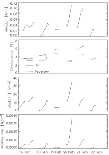
Fig. 11. Several quantities for the time interval when CHAMP was within the area 70◦<geogr. lat. < 75◦, 0◦<geogr. long. <40◦on six days of the SIRCUS campaign (16–22 February 2002). Upper panel: Hall current from the CHAMP magnetometer, second panel: conductances derived from EISCAT VHF data, third panel: magni-tude of the electric field obtained from Eq. (4), fourth panel: Joule heating rates obtained from Eq. (7).
The results are presented in Fig. 11, where the abscissa corresponds to the time interval during which CHAMP re-mained in the above stated latitude-longitude range for each day (travelling from south to north). The uppermost panel shows the magnitude of the Hall current as derived from the CHAMP magnetometer, the second panel the EISCAT-derived conductances, the third panel the electric field magni-tude derived with Eq. (4), and the lowermost panel the Joule heating rate obtained with Eq. (7). A possible neutral wind was neglected, since we have no information about it as al-ready mentioned. The conductances plotted here are the sum of the E- and the F-region contribution. The relative impor-tance of the Pedersen conductivities 6PE/6E+FP varied be-tween 0.4 and 0.6 during the intervals shown in Fig. 11, indi-cating the important contribution from the F-region, whereas the corresponding ratio for the Hall currents 6HE/6HE+F re-mained always around 0.995.
The total 6 remained between about 3 S and 6 S during all days, typical for quiet conditions.
Together with the measured Hall currents this yields elec-tric fields less than 20 mV/m for most of the time, except on 20 February where we estimated one value that exceeded 30 mV/m. We conclude that the Joule heating rates stayed below 10−3W/m2, with the exception of the one value on 20 February. As explained above, additional contributions from the F-region winds can also be expected. Since we have no handle on the neutral winds with our data set, an upper limit estimation could nevertheless be obtained from the fol-lowing considerations: for the term VFn×B a neutral wind of
the order of 300 m/s can add a contribution of 10–20 mV/m, if it flows in the proper direction. This means that we have to consider that the effective electric field may have been twice as large as the values shown in Fig. 11. This could lead to Joule heating rates of up to a factor of 4 larger than those quoted above.
Our point is however, that even if we took such a neutral wind contribution into account, the Joule heating rates would remain 1–2 orders of magnitude smaller that those observed during geomagnetic disturbed conditions when Q can exceed 0.1 W/m2(Vickrey et al., 1982; Schlegel, 1997).
In order to further check for possible Joule heating we also have examined the F-region ion temperatures. The tem-peratures were fairly constant during the observation time (08:00–12:00 UT) and did not show significant enhance-ments during the six intervals regarded in Fig. 11 with one exception: on 21 February Ti increased from about 1450 K before to 1650 K (at 430 km altitude) within the interval in question. The implication would be that some Joule heating was not showing up in Fig. 11. There was therefore perhaps a strong neutral wind contribution there.
It is absolutely not straight forward to infer possible up-welling of the atmosphere from these low heating rates. Fuller-Rowell et al. (1994) and Rishbeth et al. (1985), for instance, reported model results of upwelling for storm con-ditions, but only for altitudes below about 300 km. The for-mer quoted heating rates of up to 0.05 W/m2 as a cause. Regarding this number it seems unlikely that the large den-sity enhancements observed with CHAMP during the cor-responding passes over the cusp area can be attributed to the low heating rates of Fig. 11. It should be noted that we also made conductance estimates on two days (21 and 22 February) from measurements obtained with the EISCAT Svalbard radar using the 42-m dish (78.15◦ geogr. lat., 16.05◦ geogr. long., looking along the local field line with 81.6◦elevation), i.e. a few degrees north of the range covered with the VHF. These conductances were also around 5 S to 8 S, similar to the VHF-derived ones. Thus we do not expect very different heating rates at this latitude.
5 Summary and conclusions
Our observations (together with some earlier results based on low-resolution data) establish the existence of pronounced density structures in the high latitude thermosphere. In con-trast, the model predicts a relatively smooth density variation
at CHAMP altitudes, with none of the density structures pre-dicted for lower altitudes. The CHAMP data provide the first opportunity for detailed testing of model density pre-dictions for high altitudes (above 300 km). Furthermore, we find that the observed density structures near 430 km do not agree with the morphology of modelled thermospheric den-sity cells predicted at lower altitudes, as outlined in Sect. 3. The latter have been predicted by models for the 140–350 km altitude region at high latitudes. Their existence at these al-titudes was previously confirmed by satellite data for solar maximum and minimum conditions. The mechanisms driv-ing the cell structures in the model are still not fully under-stood. Schoendorf et al. (1996b) explained their modelled density cells as a result of thermosphere-ionosphere coupling in terms of dynamic meteorology (their Fig. 10). Caspers and Pr¨olss (1999) found moderately supporting evidence for the model results by comparing them to mass spectrometer data from the ESRO4 and DE2 satellites at heights around 200 km. These authors stress however, that they are all but convinced that the above concept of cells is correct. They of-fer an alternate explanation which is based on localized heat input.
Similar ideas have been proposed before by Taeusch and Hinton (1975, quiet conditions), Taeusch (1977, disturbed conditions). These authors examined N2 density data
ob-tained near 450 km in the polar region with a mass spec-trometer onboard OGO6. They observed local density en-hancements with a width of several 100 km and tried to re-late them to polar energy deposition. They found that the density enhancements (30–50% with respect to a model) were strongly magnetically controlled in terms of magnetic local time and magnetic latitude. For quiet conditions the density enhancements were mainly observed between 00:00 and 03:00 MLT, i.e. in the westward electrojet, and between 09:00 and 15:00 MLT, i.e. in the cusp region. During dis-turbed conditions the MLT clustering was similar but the enhancements extended further south, down to 50◦MLAT. Those authors showed polar plots that were quite similar to our Fig. 7 (apart from the density minima). For the source of local energy input they suggested soft particle precipitation in the cusp area and particle precipitation together with Joule heating in the electrojet region. Similarly Moe et al. (1977) derived a broad density bulge above 400 km near the dayside cusp from pressure gage measurements onboard the SPADES satellite, and related it to particle precipitation in this re-gion. It is interesting to note that none of the above authors ever mentioned density decreases like those we found in the CHAMP data.
Further studies are necessary to actually discriminate be-tween the various possible processes: heating by Pedersen currents associated with the strong and fast varying field aligned currents (L¨uhr et al., 2004); heating by low-energy electron precipitation which is a salient feature of the cleft re-gion; heating by proton precipitation (Frey et al., 2003). The latter authors examined soft proton precipitation in the so-called dayside proton auroral spot, a remote signature of high latitude magnetopause reconnection. Its position is within
the area where we found density enhancements. We are also unable to exclude atmospheric waves as a possible cause of the density enhancements and reductions.
Our study shows that density maxima and minima oc-curred every day during our campaign. It should be noted that apart from this very quiet period we also analysed one day with an average geomagnetic storm (not shown here). On this day too we observed the typical pattern of density maxima and minima as described here. From this limited experience it seems that this phenomenon is almost indepen-dent of geomagnetic activity. This would be consistent with a statistical study of CHAMP data taken for a whole year and which revealed only small changes in the appearance of po-lar density structures between quiet and moderate conditions (see Liu et al., 2005).
At the beginning of the paper we mentioned the possibility that part of the density excursions may be explained by neu-tral winds. Nevertheless it is fairly obvious from the present analysis that unrealistic horizontal neutral wind speeds along the satellite path exceeding 2 km/s have to be assumed in or-der to explain the data in Fig. 3, for example. Such wind speeds would only be expected during the most magnetically active conditions.
The main purpose of this study was to present the CHAMP observations and to identify the relevant patterns and charac-teristics of the density maxima/minima. More work remains to be done for a detailed explanation of the observed density structures and the mechanisms that drive them. We conclude that in spite of the fact that it has been somewhat neglected in recent experimental and modelling studies, on the basis that we “understand the thermosphere”, the upper thermosphere still seems to hold surprises.
Acknowledgements. K. Schlegel thanks the Centre for Chemical
Physics at the University of London, Ont., Canada and the Na-tional Science and Engineering Research Council of Canada for a three-month fellowship during which this work was initiated. We would like to thank P. Ritter for estimating the Hall currents from CHAMP data and W. K¨ohler for preprocessing the accelerom-eter data. The operational support of the CHAMP mission by the German Aerospace Center (DLR) and the financial support for the data processing by the Federal Ministry of Education and Research (BMBF) are gratefully acknowledged. G. Crowley was supported by AFOSR Contract F496200110059P00001, and NSF Grant ATM-0332307.
Topical Editor U.-P. Hoppe thanks J. M. Jo¨el and another referee for their help in evaluating this paper.
References
Caspers, T. and Pr¨olss, G. W.: Thermospheric density cells at high latitudes, Adv. Space Res., 24, No. 11, 1433–1437, 1999. Crowley, G., Emery, B. A., Roble, R. G., Carlson, H. C., and Knipp,
D. J.: Thermospheric dynamics during the equinox transition study I. Model simulations for Sept. 18 and 19, 1984, J. Geo-phys. Res., 94, 16 925–16 944, 1989a.
Crowley, G., Emery, B. A., Roble, R. G., Carlson, H. C., Salah, J. E., Wickwar, V. B., Miller, K. L., Oliver, W. L., Burnside, R. G.,
and Marcos, F. A.: Thermospheric dynamics during the equinox transition study of September 1994 II. Validation of the NCAR-TGCM, J. Geophys. Res., 94, 16 945–16 960, 1989b.
Crowley, G., Schoendorf, J., Roble, R. G., and Marcos, F. A.: Satel-lite observations of neutral density cells in the lower thermo-sphere at high latitudes, AGU Monograph 87 on the Mesothermo-sphere and Lower Thermosphere, 339–348, 1995.
Crowley, G., Schoendorf, J., Roble, R. G., and Marcos, F. A.: Cellu-lar structures in the high latitude lower thermosphere, J. Geophy. Res. 101, 211–223, 1996.
Frey, H. U., Phan, T. D., Fuselier, S. A., and Mende, S. B.: Con-tinuous magnetic reconnection at Earth’s magnetopause, Nature 426, 533–536, 2003.
Fuller-Rowell, T. J., Codrescu, V. M., Moffet, R. J., and Quegan, S.: Response of the thermosphere and ionosphere to geomagnetic storms, J. Geophs. Res. 99, 3893–3914, 1994.
Fuller-Rowell, T. J., Matsuo, T., Codrescu, V. M., and Marcos, F. A.: Modeling thermospheric neutral density waves and holes in response to high latitude forcing, Adv. Space Res., 24, 1447– 1458,1999.
Hedin, A. E: Extension of the MSIS thermospheric model into the middle and lower atmosphere, J. Geophys. Res. 96, 1159–1166, 1991.
Killeen, T. L., Won, Y.-I., Niciejewski, R. J., and Burns, A. G.: Upper thermosphere winds and temperatures in the geomagnetic polar cap: Solar cycle, geomagnetic activity, and interplane-tary magnetic field dependences, J. Geophys. Res., 100, 21 327– 21 342, 1995.
Liu, H., L¨uhr, H., Henize, V., and K¨ohler, W.: Global distribution of the thermospheric total mass density derived from CHAMP, J. Geophys. Res., 110, A04301, doi: 10.1029/2004JA010741, 2005.
L¨uhr, H., Rother, M., K¨ohler, W., Ritter, P., and Gr¨unwaldt, L.: Thermospheric up-welling in the cusp region, evidence from CHAMP observations, Geophys. Res. Lett., 31, L06805, doi:10.1029/2003GL019314, 2004.
Moe, K., Moe, M. M., Carter, V. L., and Ruggera, M. B.: The cor-relation of thermospheric densities with charged particle precip-itation through the magnetospheric cleft, J. Geophys. Res., 82, 3304–3306, 1977.
Pr¨olss, G. W.: Latitudinal structure and extension of the polar at-mospheric disturbance, J. Geophys. Res., 86, 2385–2396, 1981. Pr¨olss, G. W., Roemer, M., and Slowey, J. W.: Dissipation of solar
wind energy in the Earth’s upper atmosphere: The geomagnetic storm effect, Adv. Space Res., 8, (5)215–(5)261, 1988.
Rishbeth, H., Gordon, R., Rees, D., and Fuller-Rowell, T. J.: Mod-elling of thermospheric composition changes caused by a severe magnetic storm, Planet. Space Sci. 33, 1283–1301, 1985.
Ritter, P., L¨uhr, H., Viljanen, A., Amm, O., Pulkkinen, A., and Sil-lanp¨a¨a, I.: Ionospheric currents estimated simultaneously from CHAMP satellite and IMAGE ground based magnetic field mea-surements: a statistical study, Ann. Geophys., 22, 417–430, 2004,
SRef-ID: 1432-0576/ag/2004-22-417.
Richmond, A. D., Ridley, E. C., and Roble, R. G.: A thermo-sphere/ionosphere general circulation model with coupled elec-trodynamics, Geophys. Res. Lett., 19, 601–604, 1992.
Roble, R. G., Ridley, E. C., Richmond, A. D., and Dickinson, R. E.: A coupled thermosphere/ionosphere general circulation model, Geophys. Res. Lett., 15, 1325–1328, 1988.
Roble, R. G. and Ridley, E. C.: Thermosphere-Ionosphere-Mesosphere-Electro Dynamics General Circulation Model (TIME-GCM): Equinox solar cycle minimum simulations (300– 500 km), Geophys. Res. Lett., 21, 417–420, 1994.
Schlegel, K.: Auroral E-region conductivities during solar mini-mum derived from EISCAT data, Ann. Geophys., 6, 129–138, 1988.
Schlegel, K.: The use of incoherent scatter data in ionospheric and plasma research, in: Incoherent Scatter–Theory Practice and Sci-ence, edited by: Alcayd´e, D., EISCAT Scientific Assoc., Kiruna, Sweden, 89–120, 1997.
Schoendorf, J. and Crowley, G.: Interpretation of an unusual high latitude density decrease in terms of thermospheric density cells, Geophys. Res. Lett., 22, 3023–3026, 1995.
Schoendorf, J., Crowley, G., and Roble, R. G.: Neutral density cells in the high latitude thermosphere – 1. Solar maximum cell mor-phology and data analysis, J. Atmos. Terr. Phys. 58, 1751–1768, 1996a.
Schoendorf, J., Crowley, G., and Roble, R. G.: Neutral density cells in the high latitude thermosphere – 2. Mechanisms, J. Atmos. Terr. Phys. 58, 1769–1781, 1996b.
Taeusch, D. R.: Structure of electrodynamic and particle heating in the disturbed polar thermosphere, J. Geophys. Res., 82, 455–460, 1977.
Taeusch, D. R. and Hinton, B. B.: Structure of electrodynamic and particle heating in the undisturbed polar thermosphere, J. Geo-phys. Res., 80, 4346–4350, 1975.
Vickrey, J.,F., Wondrak, R. R., and Mathews, S. J.: Energy deposi-tion by precipitating particles and Joule dissipadeposi-tion in the auroral ionosphere, J. Geophys. Res. 87, 5184–5196, 1982.
Watermann, J., L¨uhr, H., Schlegel, K., Stauning, P., Thayer, J. P., Christiansen, F., and Newell, P. T.: The low-altitude cusp: multi-point observations during the February 2002 SIRCUS campaign, in: Earth Observation with CHAMP: Results from Three Years in Orbit, edited by: Reigber, C., L¨uhr, H., Schwintzer, P., and Wickert, J., Springer, Berlin–Heidelberg, 375–380, 2005.