Long range time transfer over optical fiber links and cross-comparison with satellite based methods.

Texte intégral

(1)Long range time transfer over optical fiber links and cross-comparison with satellite based methods. Namneet Kaur. To cite this version: Namneet Kaur. Long range time transfer over optical fiber links and cross-comparison with satellite based methods.. Physics [physics]. SYRTE, Observatoire de Paris, 2018. English. �tel-01913286�. HAL Id: tel-01913286 https://hal.archives-ouvertes.fr/tel-01913286 Submitted on 6 Nov 2018. HAL is a multi-disciplinary open access archive for the deposit and dissemination of scientific research documents, whether they are published or not. The documents may come from teaching and research institutions in France or abroad, or from public or private research centers.. L’archive ouverte pluridisciplinaire HAL, est destinée au dépôt et à la diffusion de documents scientifiques de niveau recherche, publiés ou non, émanant des établissements d’enseignement et de recherche français ou étrangers, des laboratoires publics ou privés..

(2) THÈSE DE DOCTORAT de l’Université de recherche Paris Sciences et Lettres PSL Research University. Préparée à SYRTE, Observatoire de Paris. Transfert de temps à longue distance utilisant des liaisons à fibre optique et comparaison croisée avec des méthodes par satellite École doctorale no 127 ASTRONOMIE ET ASTROPHYSIQUE D’ILE-DE-FRANCE. Spécialité. ASTRONOMIE ET ASTROPHYSIQUE. COMPOSITION DU JURY :. Mme Fabienne Casoli, Président LERMA, Observatoire de Paris M François Vernotte, Rapporteur Observatire de Besançon Mme Catherine Algani, Rapporteur CNAM, Paris. Soutenue par Namneet KAUR le 20 Avril 2018. M Javier Díaz, Membre du jury University of Granada, Spain M Jean Pierre Aubry, Membre du jury Établissement M Philip Tuckey, Directeur de thése SYRTE, Observatoire de Paris M Paul-Eric Pottie, Co-supervisor de thése SYRTE, Observatoire de Paris.

(3)

(4) i. Acknowledgements. I am heartily thankful to my supervisors for their immense help and support. Their enlightening discussions and constant motivation have been the guiding light throughout the journey of my thesis. In addition to the rich professional learning experience that I have gained while working with them, the time spent with them has strengthened and shaped my personality. I wish to express my deep gratitude for their generosity, affection, and understanding. It has been an honor and an absolute pleasure to work with them and I am very grateful for this life-changing opportunity. I would like to thank Javier Diaz, Rafa Rogriguez, J. Gabriel Ramirez at Seven Solutions and Felipe Torres Gonzalez at University of Granada, Spain for their collaboration and support. I would also like to thank the White Rabbit community for their help by sharing issues through the mailing list and would like to specially thank Javier Serrano, Alessandro Rubini, T. Wlostowski and Mattia Rizzi at CERN for their help and support. I would also take the opportunity to thank Noel Dimarcq for his stimulating conversations and goodwill. I would specially like to thank the members of SYRTE belonging to Time and Frequency group, Electronics group, Computing group, Fiber link group and administration for their continuous help, support and for their valuable time for urgent matters. I extend my profound gratitude to my Mom and Dad for being my ever increasing strength and motivation. I would also like to acknowledge my family and all my dearest friends, specially Navnina and Vishnu for being my backbone and for always being there in difficult times. I am truly grateful and I cherish their invaluable friendship. This work was supported by the LABEX Cluster of Excellence FIRST-TF (ANR10-LABX-48-01), within the Program d’Investissements d’Avenir and by BPIFrance under the SCP Time project..

(5)

(6) iii. I dedicate this thesis to my Mom and Dad..

(7)

(8) v. Contents Acknowledgements. i. 1. Introduction. 1. 1.1. Time and frequency metrology . . . . . . . . . . . . . . . . . . . . . . .. 1. 1.1.1. Accuracy . . . . . . . . . . . . . . . . . . . . . . . . . . . . . . . .. 1. 1.1.2. Stability . . . . . . . . . . . . . . . . . . . . . . . . . . . . . . . .. 2. 1.2. The Oscillator signal . . . . . . . . . . . . . . . . . . . . . . . . . . . . .. 2. 1.3. Noise analysis . . . . . . . . . . . . . . . . . . . . . . . . . . . . . . . . .. 3. 1.3.1. Frequency domain . . . . . . . . . . . . . . . . . . . . . . . . . .. 3. 1.3.2. Time domain . . . . . . . . . . . . . . . . . . . . . . . . . . . . .. 4. 1.3.2.1. Allan Variance . . . . . . . . . . . . . . . . . . . . . . .. 4. 1.3.2.2. Overlapping Allan Variance . . . . . . . . . . . . . . .. 5. 1.3.2.3. Modified Allan Variance . . . . . . . . . . . . . . . . .. 5. 1.3.2.4. Time Variance . . . . . . . . . . . . . . . . . . . . . . .. 5. 1.4. Clocks and timescales . . . . . . . . . . . . . . . . . . . . . . . . . . . .. 6. 1.5. Introduction to time transfer methods . . . . . . . . . . . . . . . . . . .. 8. 1.5.1. One way time transfer method . . . . . . . . . . . . . . . . . . .. 8. 1.5.1.1. GNSS time dissemination . . . . . . . . . . . . . . . . .. 9. 1.5.1.2. GNSS time transfer methods . . . . . . . . . . . . . . . 10. 1.5.2. Two way time transfer method . . . . . . . . . . . . . . . . . . . 11. 1.5.3. Two way Satellite Time and Frequency transfer (TWSTFT) . . . 13. 1.5.4. Time and frequency transfer over Optical fiber links . . . . . . . 15. 1.5.5. Time over Internet . . . . . . . . . . . . . . . . . . . . . . . . . . 16. 1.5.6 1.6. 1.7. 1.5.5.1. Network Time Protocol (NTP) . . . . . . . . . . . . . . 16. 1.5.5.2. Precision Time Protocol . . . . . . . . . . . . . . . . . . 17. 1.5.5.3. SONET and SDH . . . . . . . . . . . . . . . . . . . . . 18. 1.5.5.4. White Rabbit PTP (WR-PTP) . . . . . . . . . . . . . . . 18. Performance comparison of some time transfer methods . . . . 19. Implemented and Potential applications of White Rabbit . . . . . . . . 20 1.6.1. For Scientific experiments . . . . . . . . . . . . . . . . . . . . . . 20. 1.6.2. Calibration in the RF domain . . . . . . . . . . . . . . . . . . . . 21. 1.6.3. Smart power grids . . . . . . . . . . . . . . . . . . . . . . . . . . 21. 1.6.4. 5G mobile networks . . . . . . . . . . . . . . . . . . . . . . . . . 21. 1.6.5. Financial transactions and timestamping . . . . . . . . . . . . . 21. Outline of the thesis . . . . . . . . . . . . . . . . . . . . . . . . . . . . . . 21.

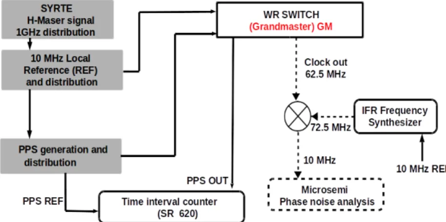
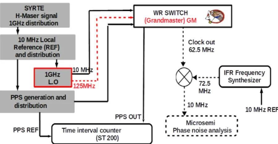
(9) vi 2. Introduction to White Rabbit Precision Time Protocol (WR-PTP). 23. 2.1. Introduction to WR project . . . . . . . . . . . . . . . . . . . . . . . . . . 23. 2.2. Introduction to WR-PTP . . . . . . . . . . . . . . . . . . . . . . . . . . . 23 2.2.1. Precision time Protocol (PTP) . . . . . . . . . . . . . . . . . . . . 23. 2.2.2. Synchronous Ethernet . . . . . . . . . . . . . . . . . . . . . . . . 26. 2.2.3. Digital Dual Mixer time difference (DDMTD) phase detector . . 26. 2.3. A typical White Rabbit Network . . . . . . . . . . . . . . . . . . . . . . 28. 2.4. Synchronization in White Rabbit . . . . . . . . . . . . . . . . . . . . . . 29 2.4.1. Syntonization . . . . . . . . . . . . . . . . . . . . . . . . . . . . . 30. 2.4.2. Link Delay measurement . . . . . . . . . . . . . . . . . . . . . . 30. 2.4.3. Link asymmetry evaluation . . . . . . . . . . . . . . . . . . . . . 31. 2.4.4. Clock offset evaluation . . . . . . . . . . . . . . . . . . . . . . . . 34. 2.5. Unification of White Rabbit into PTP . . . . . . . . . . . . . . . . . . . . 34. 2.6. Components of a White Rabbit Network . . . . . . . . . . . . . . . . . . 35. 2.7. White Rabbit equipment . . . . . . . . . . . . . . . . . . . . . . . . . . . 35 2.7.1. The White Rabbit Switch . . . . . . . . . . . . . . . . . . . . . . . 35. 2.7.2. The White Rabbit Nodes . . . . . . . . . . . . . . . . . . . . . . . 36. 2.8. Optical emitters . . . . . . . . . . . . . . . . . . . . . . . . . . . . . . . . 37. 2.9. The transmission medium - Optical fibers . . . . . . . . . . . . . . . . . 38. 2.10 White Rabbit clocking Scheme . . . . . . . . . . . . . . . . . . . . . . . . 41 2.11 The potential performance limitations . . . . . . . . . . . . . . . . . . . 42 2.12 Outlook . . . . . . . . . . . . . . . . . . . . . . . . . . . . . . . . . . . . . 45 3. Improving the White Rabbit Switch performance. 47. 3.1. Introduction . . . . . . . . . . . . . . . . . . . . . . . . . . . . . . . . . . 47. 3.2. The White Rabbit Switch in Grandmaster mode . . . . . . . . . . . . . 47. 3.3. 3.4. 3.5. 3.2.1. Experimental setup . . . . . . . . . . . . . . . . . . . . . . . . . . 47. 3.2.2. Phase noise power spectral density . . . . . . . . . . . . . . . . . 48. Improving the Grandmaster WRS performance . . . . . . . . . . . . . . 49 3.3.1. Phase noise Power Spectral Density and Allan Deviation . . . . 50. 3.3.2. Time Stability performance . . . . . . . . . . . . . . . . . . . . . 53. Performance of a Slave White Rabbit Switch. . . . . . . . . . . . . . . . 55. 3.4.1. Testing Optical link configurations . . . . . . . . . . . . . . . . . 55. 3.4.2. Experimental setup . . . . . . . . . . . . . . . . . . . . . . . . . . 55. 3.4.3. Effect of Chromatic dispersion . . . . . . . . . . . . . . . . . . . 56. 3.4.4. Results . . . . . . . . . . . . . . . . . . . . . . . . . . . . . . . . . 58. Improving the performance of a Slave WRS . . . . . . . . . . . . . . . . 60 3.5.1. Phase Locked Loops (PLL) . . . . . . . . . . . . . . . . . . . . . 60. 3.5.2. Experimental Setup . . . . . . . . . . . . . . . . . . . . . . . . . . 62. 3.5.3. Phase locked loop Bandwidth variation . . . . . . . . . . . . . . 62. 3.5.4. A mid range White Rabbit link . . . . . . . . . . . . . . . . . . . 65. 3.5.5. Phase locked loop bandwidth optimization . . . . . . . . . . . . 65.

(10) vii 3.5.6. 4. 3.6. The Local Oscillator performance . . . . . . . . . . . . . . . . . . . . . . 68. 3.7. Increasing the PTP message exchange rate . . . . . . . . . . . . . . . . . 70. 3.8. Summary . . . . . . . . . . . . . . . . . . . . . . . . . . . . . . . . . . . . 72. Towards long range time and frequency dissemination using White Rabbit 74 4.1. Introduction . . . . . . . . . . . . . . . . . . . . . . . . . . . . . . . . . . 74. 4.2. A realistic Telecommunication network span . . . . . . . . . . . . . . . 74 Experimental Setup . . . . . . . . . . . . . . . . . . . . . . . . . . 74. 4.2.2. Phase locked loop Bandwidth optimization . . . . . . . . . . . . 75. 4.2.3. Experimental results . . . . . . . . . . . . . . . . . . . . . . . . . 76. 4.2.4. Fiber thermal noise . . . . . . . . . . . . . . . . . . . . . . . . . . 78. 4.2.5. Limitations for the time stability performance . . . . . . . . . . 81. Effect of Chromatic Dispersion . . . . . . . . . . . . . . . . . . . . . . . 82. 4.4. Tackling Chromatic Dispersion . . . . . . . . . . . . . . . . . . . . . . . 84. 4.5. Cascaded White Rabbit links using DWDM technique . . . . . . . . . . 85. 4.7. 4.8. 6. 4.2.1. 4.3. 4.6. 5. Frequency and Time stability performance . . . . . . . . . . . . 67. 4.5.1. Experimental Setup . . . . . . . . . . . . . . . . . . . . . . . . . . 85. 4.5.2. Phase locked loop Bandwidth optimization for cascaded stages. 4.5.3. Frequency and time stability performance . . . . . . . . . . . . 90. 4.5.4. Extension to a Cascaded 400 km White Rabbit link . . . . . . . . 91. 86. 4.5.4.1. Phase locked loop bandwidth optimization . . . . . . 93. 4.5.4.2. Frequency stability performance . . . . . . . . . . . . . 93. 4.5.4.3. Time stability performance . . . . . . . . . . . . . . . . 94. A long haul telecommunication span White Rabbit link . . . . . . . . . 98 4.6.1. Experimental setup . . . . . . . . . . . . . . . . . . . . . . . . . . 98. 4.6.2. Frequency stability performance . . . . . . . . . . . . . . . . . . 99. 4.6.3. Time stability performance . . . . . . . . . . . . . . . . . . . . . 101. 4.6.4. Effect of reduced PTP rate . . . . . . . . . . . . . . . . . . . . . . 105. 4.6.5. Effect of reduced Bandwidth of locking . . . . . . . . . . . . . . 107. A multi user 4x125 km White Rabbit link . . . . . . . . . . . . . . . . . 110 4.7.1. Experimental Setup . . . . . . . . . . . . . . . . . . . . . . . . . . 110. 4.7.2. Frequency and time stability performance . . . . . . . . . . . . 111. Conclusion . . . . . . . . . . . . . . . . . . . . . . . . . . . . . . . . . . . 113. Deployments. 116. 5.1. Introduction . . . . . . . . . . . . . . . . . . . . . . . . . . . . . . . . . . 116. 5.2. A short range in-campus dissemination network . . . . . . . . . . . . . 116. 5.3. A mid range suburban WR link using dark fiber network . . . . . . . . 117. Time Accuracy. 118. 6.1. Introduction . . . . . . . . . . . . . . . . . . . . . . . . . . . . . . . . . . 118. 6.2. Calibration of fiber spools using White Rabbit . . . . . . . . . . . . . . 119 6.2.1. Calibration: A sensitive task . . . . . . . . . . . . . . . . . . . . . 120.

(11) viii 6.2.2 6.3. Wavelength swapping technique . . . . . . . . . . . . . . . . . . . . . . 126 6.3.1. 6.4. 7. Implementation and Results . . . . . . . . . . . . . . . . . . . . 129. Dual wavelength technique . . . . . . . . . . . . . . . . . . . . . . . . . 130 6.5.1. 6.6. Implementation and Results . . . . . . . . . . . . . . . . . . . . 127. Fiber swapping technique . . . . . . . . . . . . . . . . . . . . . . . . . . 128 6.4.1. 6.5. Calibration by forcing asymmetry in a uni-directional link . . . 120. Implementation and Results . . . . . . . . . . . . . . . . . . . . 134. Summary . . . . . . . . . . . . . . . . . . . . . . . . . . . . . . . . . . . . 137. Conclusion. 139. 7.1. Summary . . . . . . . . . . . . . . . . . . . . . . . . . . . . . . . . . . . . 139. 7.2. Perspectives . . . . . . . . . . . . . . . . . . . . . . . . . . . . . . . . . . 141. A. 143. Bibliography. 153.

(12) ix. List of Figures 1.1. The relationship between accuracy and stability for a frequency standard of nominal frequency f 0 [1]. . . . . . . . . . . . . . . . . . . . . . .. 1.2. 2. The time evolution of the uncertainty of Cesium and Optical clocks. Fractional uncertainty of primary Cesium atomic clocks to realize the second in the SI (squares) and optical frequency clocks (dots). Green dots represent optical clocks with estimated standard uncertainties whose optical frequency can be determined only with the accuracy of the frequency comparison with a primary Cesium clock [7]. . . . . .. 7. 1.3. One way time and frequency transfer. . . . . . . . . . . . . . . . . . . .. 8. 1.4. One way time and frequency transfer. . . . . . . . . . . . . . . . . . . .. 9. 1.5. GPS common-view technique [10]. . . . . . . . . . . . . . . . . . . . . . 10. 1.6. General schematic of a two way time transfer method. . . . . . . . . . . 12. 1.7. Two way satellite time and frequency transfer [18]. . . . . . . . . . . . . 14. 1.8. NTP two way message exchange process. . . . . . . . . . . . . . . . . . 17. 1.9. WR synchronization performance for initial experiments by CERN[42]. 19. 1.10 Performance comparison of some time transfer methods. . . . . . . . . 20 2.1. PTP two way messsage exchange mechanism [39]. . . . . . . . . . . . . 25. 2.2. Comparison between Standard and Synchronous Ethernet [56]. . . . . 26. 2.3. Schematic of an analog DMTD phase detector [56] . . . . . . . . . . . . 27. 2.4. Schematic of a digital DMTD phase detector [56]. . . . . . . . . . . . . . 28. 2.5. A typical White Rabbit Network [42]. . . . . . . . . . . . . . . . . . . . . 29. 2.6. A White Rabbit link delay scheme [56]. . . . . . . . . . . . . . . . . . . . 30. 2.7. Delay asymmetries in a White Rabbit link [56]. . . . . . . . . . . . . . . 31. 2.8. White Rabbit transceiver PHY calibration scheme [56]. . . . . . . . . . 32. 2.9. WR-PTP message exchange flow [56]. . . . . . . . . . . . . . . . . . . . 35. 2.10 A White Rabbit Switch (WRS) [59]. . . . . . . . . . . . . . . . . . . . . . 36 2.11 SPEC board hosting the five channel FMC card DIO [60]. . . . . . . . . 37 2.12 The White Rabbit Zync embedded node (WR-ZEN) [61]. . . . . . . . . 38 2.13 Types of Small form factor pluggable (SFP) optical transceivers. . . . . 38 2.14 Optical attenuation variation with wavelength [63]. . . . . . . . . . . . 39 2.15 Refractive index, group index and material dispersion of silica fibers [63]. . . . . . . . . . . . . . . . . . . . . . . . . . . . . . . . . . . . . . . . 40 2.16 Clocking scheme of the White Rabbit switch hardware v3.4v (v3.3 lacks the 10 MHz clock output) [71]. . . . . . . . . . . . . . . . . . . . . 42.

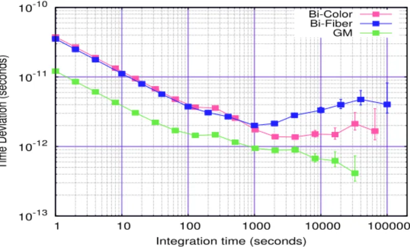
(13) x 2.17 Illustration of a typical Phase noise power spectral density for a free running local oscillator, for the external reference signal and for the locked local oscillator. . . . . . . . . . . . . . . . . . . . . . . . . . . . . 43 2.18 A WR Slave system review for studying its potential performance limitations [71]. . . . . . . . . . . . . . . . . . . . . . . . . . . . . . . . . . . 44 2.19 Pictorial representation of the potential noise sources that could limit the frequency stability performance of a typical Grandmaster and Slave White Rabbit Switch. . . . . . . . . . . . . . . . . . . . . . . . . . . . . . 45 3.1. Experimental setup for GM switch performance analysis. . . . . . . . . 48. 3.2. Phase noise power spectral density for the Grandmaster WR clock. . . 48. 3.3. Schematic of the external 1 GHz local oscillator box. . . . . . . . . . . . 49. 3.4. Phase noise power spectral density of the 10 MHz output signal of the 1 GHz local oscillator box. . . . . . . . . . . . . . . . . . . . . . . . . . . 50. 3.5. Experimental setup for the "improved" GM switch performance analysis. . . . . . . . . . . . . . . . . . . . . . . . . . . . . . . . . . . . . . . . 51. 3.6. Phase noise power spectral density for default and improved Grandmaster WR clock. . . . . . . . . . . . . . . . . . . . . . . . . . . . . . . . 51. 3.7. Phase noise power spectral density of the improved Grandmaster WR clock for PLL bandwidth optimization. . . . . . . . . . . . . . . . . . . 52. 3.8. Allan Deviation (NEQ BW=500 Hz) for default and Improved Grandmaster WR clock (the solid light blue and red lines are their respective noise floors). . . . . . . . . . . . . . . . . . . . . . . . . . . . . . . . . . . 52. 3.9. Comparison of Allan Deviation (NEQ BW=50 Hz) of our Improved Grandmaster WRS with OPNT enhanced WR. . . . . . . . . . . . . . . 53. 3.10 Phase data for the improved Grandmaster WRS (constant offset has been removed). . . . . . . . . . . . . . . . . . . . . . . . . . . . . . . . . 53 3.11 Time Deviation for default and Improved Grandmaster switch (Bandwidth of measurement = 1 Hz). . . . . . . . . . . . . . . . . . . . . . . . 54 3.12 Experimental setup for comparison of uni-directional (Bi-fiber) and bi-directional (Bi-color) 25 km White Rabbit links. . . . . . . . . . . . . 56 3.13 Optical spectrum of the 1310 and 1490 nm (Bi-directional) CWDM SFPs. 57 3.14 Optical spectrum of the 1541 and 1560 nm (Uni-directional) DWDM SFPs. . . . . . . . . . . . . . . . . . . . . . . . . . . . . . . . . . . . . . . 57 3.15 Phase data for the uni-directional (Bi-fiber) and bi-directional (Bi-color) setups. . . . . . . . . . . . . . . . . . . . . . . . . . . . . . . . . . . . . . 59 3.16 Overlapping Allan Deviation (calculated from phase data) for the unidirectional and bidirectional setups (Bandwidth of measurement = 1 Hz). . . . . . . . . . . . . . . . . . . . . . . . . . . . . . . . . . . . . . . 59 3.17 Time Deviation (calculated from phase data) for the unidirectional and bidirectional setups (Bandwidth of measurement = 1 Hz). . . . . . 60 3.18 Block diagram of a typical phase locked loop [81]. . . . . . . . . . . . . 61.

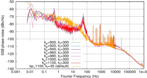
(14) xi 3.19 Experimental setup for a 25 km White Rabbit uni-directional link. . . . 62 3.20 Power spectral density of the Slave clock for different k p values for a constant k i =30. . . . . . . . . . . . . . . . . . . . . . . . . . . . . . . . . 63 3.21 Power spectral density of the Slave clock for different k i values for a constant k p =800. . . . . . . . . . . . . . . . . . . . . . . . . . . . . . . . 64 3.22 Power spectral density of the Slave clock for different k p values for a constant k i =300. . . . . . . . . . . . . . . . . . . . . . . . . . . . . . . . . 64 3.23 Experimental setup for a 50 km White Rabbit uni-directional link. . . . 65 3.24 Power spectral density of the Slave clock for fine tuning of k p values for a constant k i =300. . . . . . . . . . . . . . . . . . . . . . . . . . . . . . 66 3.25 Allan deviation (NEQ BW=50 Hz) for the Slave switch for default and optimized gain parameters. . . . . . . . . . . . . . . . . . . . . . . . . . 66 3.26 Phase data of the Slave WRS for the 50 km WR link (constant offset has been removed). . . . . . . . . . . . . . . . . . . . . . . . . . . . . . . 67 3.27 Frequency stability for a 50 km White Rabbit link. . . . . . . . . . . . . 67 3.28 Time Deviation for a 50 km White Rabbit link. . . . . . . . . . . . . . . 68 3.29 Relative frequency noise for the Slave switch, error signal of the Slave switch and for the local oscillator of the WRS. . . . . . . . . . . . . . . . 69 3.30 Relative frequency noise contribution from the 3.3 V and 5 V internal power supply, for the Grandmaster and the Slave switch. . . . . . . . . 70 3.31 Frequency stability (calculated from phase data) comparison for default and increased PTP rate for the Slave WRS (100 km link). . . . . . 72 4.1. Experimental setup for a 100 km White Rabbit uni-directional link. . . 75. 4.2. Phase noise power spectral density of the Slave clock for k p =4000 and k i values. . . . . . . . . . . . . . . . . . . . . . . . . . . . . . . . . . . . . 76. 4.3. Allan Deviation of the Slave clock for different k p and k i values. . . . . 77. 4.4. Phase data for the two Slaves (constant offset removed). . . . . . . . . . 77. 4.5. Overlapping Allan deviation (calculated from phase data) for the 100 km uni-directional WR link. . . . . . . . . . . . . . . . . . . . . . . . . . . . 78. 4.6. Time deviation (calculated from phase data) for the 100 km uni-directional WR link. . . . . . . . . . . . . . . . . . . . . . . . . . . . . . . . . . . . . 79. 4.7. Ambient temperature variations experienced and recorded by the time interval counter STS201 and the calculated phase fluctuations. The green trace is the Slave switch data as in Fig. 4.4. We observe a compression factor of about 5 at half a day. . . . . . . . . . . . . . . . . . . . 80. 4.8. Overlapping Allan deviation (calculated from phase data) for the 100 km uni-directional WR link with evidence of the fiber thermal noise bump. 81. 4.9. Limitations for the time stability (calculated from phase data) performance of the 100 km White Rabbit link. . . . . . . . . . . . . . . . . . . 82. 4.10 Chromatic dispersion contribution to the time stability performance of the Slave switch (100 km telecom span uni-directional link). . . . . . 83.

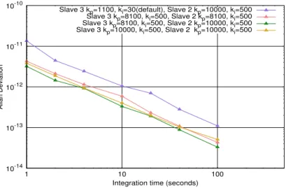
(15) xii 4.11 Experimental setup for the cascaded 300 km White Rabbit link. . . . . 86 4.12 Phase noise power spectral density of the Second Slave clock for different k p values with constant k i =500. . . . . . . . . . . . . . . . . . . . 87 4.13 Phase noise power spectral density of the third Slave clock for default gain values and different k p values for constant k i =500. . . . . . . . . . 87 4.14 Allan Deviation (NEQ BW=5 Hz) for the third Slave clock for default gain values and higher k p values for constant k i =500. . . . . . . . . . . 88 4.15 Phase noise power spectral density comparison for the cascaded stages. 89 4.16 Allan Deviation (NEQ BW=500 Hz) for the cascaded stages. . . . . . . 89 4.17 Phase data for the 200 and 300 km cascaded stages (constant offset removed). . . . . . . . . . . . . . . . . . . . . . . . . . . . . . . . . . . . 90 4.18 Overlapping Allan Deviation (calculated from the phase data) for the 200 and 300 km cascaded stages. . . . . . . . . . . . . . . . . . . . . . . 91 4.19 Time Deviation (calculated from the phase data) for the 200 and 300 km cascaded stages. . . . . . . . . . . . . . . . . . . . . . . . . . . . . . . . . 91 4.20 Experimental setup for the cascaded 400 km White Rabbit link. . . . . 92 4.21 Relative frequency deviation for each of the cascaded stages of the 400 km cascaded White Rabbit link. . . . . . . . . . . . . . . . . . . . . 93 4.22 Overlapping Allan Deviation (calculated from frequency data) for the 400 km cascaded White Rabbit link. . . . . . . . . . . . . . . . . . . . . 94 4.23 Phase data for the cascaded 300 km stage and for the user end node at 400 km (constant offset removed). . . . . . . . . . . . . . . . . . . . . 94 4.24 Time Deviation calculated from the phase data for the 300 km cascaded stage and for the user end node at 400 km. . . . . . . . . . . . . . 95 4.25 Phase data measurement for the 300 and 400 km cascaded link for the test of short term stability limitation. . . . . . . . . . . . . . . . . . . . . 96 4.26 Comparison of Overlapping Allan Deviation (calculated from phase data) for the 300 and 400 km cascaded stages for counter swapped case. 96 4.27 Comparison of Time Deviation (calculated from phase data) for the 300 and 400 km cascaded stages for counter swapped case. . . . . . . . 97 4.28 Time stability comparison for the frequency data and phase data for the 400 km cascaded link. . . . . . . . . . . . . . . . . . . . . . . . . . . 97 4.29 Experimental setup for the cascaded 500 km White Rabbit link. . . . . 98 4.30 Relative frequency deviation for each of the cascaded stages of the 500 km White Rabbit link with increased PTP rate and increased BW of locking. . . . . . . . . . . . . . . . . . . . . . . . . . . . . . . . . . . . 100 4.31 Allan Deviation for the 500 km cascaded White Rabbit link and comparison with different GPS receivers. Solid line depicts stability calculated from Frequency data, Dashed line depicts stability calculated from Phase data. . . . . . . . . . . . . . . . . . . . . . . . . . . . . . . . . 101.

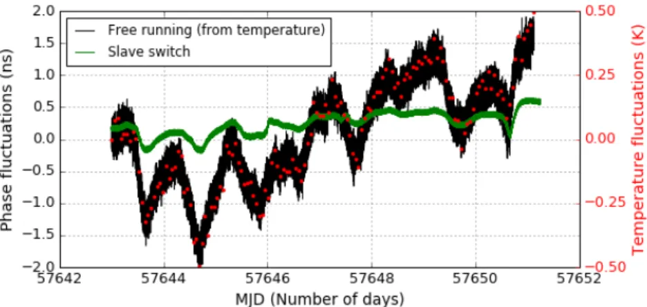
(16) xiii 4.32 Top: Free running phase fluctuations calculated from the temperature fluctuations of the experimental room (constant offset removed for both), and the Slave ZEN phase fluctuations (blue trace). The blue trace is zoomed in the bottom figure. We observe a compression factor of about 20. . . . . . . . . . . . . . . . . . . . . . . . . . . . . . . . . . . . 102 4.33 Time stability (calculated from phase data) for the cascaded 500 km White Rabbit link and comparison with infield applications. . . . . . . 103 4.34 Time stability calculated from the frequency data for the cascaded 500 km White Rabbit link. . . . . . . . . . . . . . . . . . . . . . . . . . . 104 4.35 Wavelength fluctuations for the 1541 nm SFP (constant offset removed).104 4.36 Relative frequency deviation for each of the cascaded stages of the 500 km White Rabbit link with default PTP rate. . . . . . . . . . . . . . 105 4.37 Allan Deviation (calculated from frequency data) for the 500 km cascaded White Rabbit link for default PTP rate. . . . . . . . . . . . . . . . 106 4.38 Time stability calculated from the frequency data for the cascaded 500 km White Rabbit link for default PTP rate. . . . . . . . . . . . . . . 107 4.39 Relative frequency deviation for each of the cascaded stages of the 500 km White Rabbit link with default bandwidth of locking and default PTP rate. . . . . . . . . . . . . . . . . . . . . . . . . . . . . . . . . . 108 4.40 Allan Deviation (calculated from frequency data) for the 500 km cascaded White Rabbit link for default bandwidth of locking along with default PTP rate. . . . . . . . . . . . . . . . . . . . . . . . . . . . . . . . . 109 4.41 Time stability calculated from the frequency data for the cascaded 500 km White Rabbit link for default bandwidth of locking along with default PTP rate. . . . . . . . . . . . . . . . . . . . . . . . . . . . . . . . . 109 4.42 Time stability comparison calculated from phase data for the cascaded 500 km White Rabbit link for default bandwidth of locking along with default PTP rate. . . . . . . . . . . . . . . . . . . . . . . . . . . . . . . . . 110 4.43 Experimental setup for the multi user 125 km White Rabbit link. . . . . 110 4.44 Relative frequency deviation for each of the Slaves at 125 km . . . . . . 111 4.45 Allan Deviation (calculated from frequency data) for the multi-user 4x125 km White Rabbit links. . . . . . . . . . . . . . . . . . . . . . . . . 112 4.46 Time Deviation calculated from frequency data for the multi-user 4x125 km White Rabbit links. . . . . . . . . . . . . . . . . . . . . . . . . . . . . . . 112 4.47 Pictorial representation of the short term and long term limitations for time stability performance of a long haul White Rabbit link. . . . . . . 113 5.1. Experimental setup of the UTC room to Laboratory White Rabbit link. 116. 5.2. A 43 km suburban telecommunication network White Rabbit link between SYRTE and LPL (Université Paris 13), Paris. . . . . . . . . . . . . 117. 6.1. Experimental setup for the calibration of the fiber spool. . . . . . . . . 120.

(17) xiv 6.2. Variation of the delay (offset has been removed) for connecting/disconnecting the fiber link. . . . . . . . . . . . . . . . . . . . . . . . . . . . . . . . . . . 121. 6.3. Experimental setup of the UTC room to Laboratory White Rabbit link. 127. 6.4. A 43 km sub-urban active telecommunication network White Rabbit link between SYRTE and LPL (Université Paris 13), Paris. . . . . . . . . 129. 6.5. The two way PTP scheme for dual wavelength technique. . . . . . . . 130. 6.6. The two way PTP scheme for dual wavelength technique with Thales theorem representation. . . . . . . . . . . . . . . . . . . . . . . . . . . . 131. 6.7. Experimental setup for a 125 km White Rabbit uni-directional link for two Slave WRS. . . . . . . . . . . . . . . . . . . . . . . . . . . . . . . . . 134. 6.8. Round trip time fluctuations for both the Slaves over 16 days of measurement (offset has been removed for both). The trace for Slave 2 has been shifted by 2 ns for clarity. . . . . . . . . . . . . . . . . . . . . . . . 135. 6.9. Fluctuations of the round trip time difference Slave2-Slave1 (offset has been removed). . . . . . . . . . . . . . . . . . . . . . . . . . . . . . . . . 136. 6.10 Fluctuations of β over 16 days of measurement. . . . . . . . . . . . . . . 136.

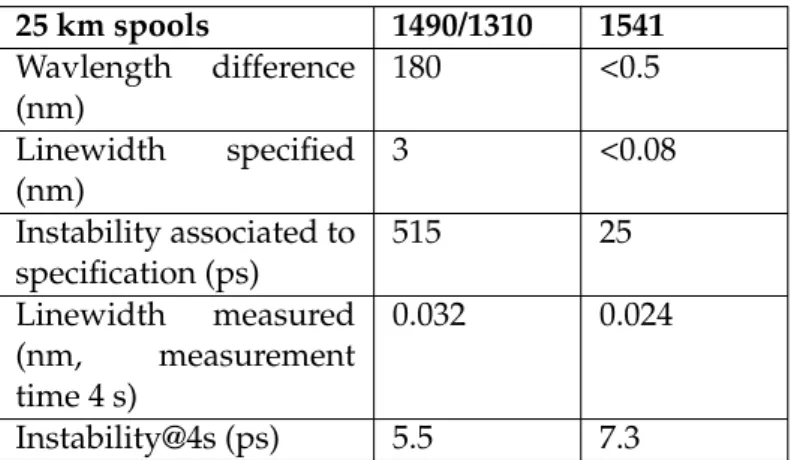
(18) xv. List of Tables 1.1. Characterization of different noise types for a typical oscillator [2]. PM-Phase modulation, FM- Frequency modulation. . . . . . . . . . . .. 1.2. Different noise processes and their dependence on α and τ in the frequency and time domain respectively. . . . . . . . . . . . . . . . . . . .. 3.1. 3 6. Comparison of the effect of Chromatic Dispersion on stability for commercial SFPs in two setups: a bi-color link using 1490/1310 nm emitters and a single fiber, and a bi-fiber link using the DWDM emitters at 1541 nm and dual fibers. . . . . . . . . . . . . . . . . . . . . . . . . . . . 58. 3.2. Summary of the main results. . . . . . . . . . . . . . . . . . . . . . . . . 73. 4.1. Allan Deviation (62.5 MHz) at one second of integration time for the Slave clock for different k p and k i values. . . . . . . . . . . . . . . . . . 76. 4.2. Comparison of the optimized set of gain parameters for increasing link length. . . . . . . . . . . . . . . . . . . . . . . . . . . . . . . . . . . . 88. 4.3. Summary of the main results. ADEV-Allan Deviation, ODAEV- Overlapping ADEV, TDEV- Time deviation. * the stability is calculated from K+K frequency counter data, else the stability is calculated from time interval counter data. . . . . . . . . . . . . . . . . . . . . . . . . . . 115. 6.1. The measured round trip time (RTT) and bitslide values for Step 1, 2, 3. 122. 6.2. The calculated propagation delay for the fiber spool 1 from step 2,3 and the corresponding calculated length of the fiber spool. . . . . . . . 123. 6.3. Time interval counter readings for Step 1, 2, 3 for Spool 1. . . . . . . . . 124. 6.4. The measured round trip time (RTT) and bitslide values for Step 1, 2, 3 for Spool 2. . . . . . . . . . . . . . . . . . . . . . . . . . . . . . . . . . . 125. 6.5. The calculated propagation delay for the fiber spool from step 2,3 and the corresponding calculated length of the fiber spool for Spool 2. . . . 125. 6.6. Time interval counter readings for Step 1, 2, 3 for Spool 2. . . . . . . . . 126. 6.7. Wavelength swapping of the two links and corresponding variation of δ values. . . . . . . . . . . . . . . . . . . . . . . . . . . . . . . . . . . . 128.

(19) xvi. List of Abbreviations BC. Boundary clock. CWDM. Coarse Wavelength Division Multiplexing. DAC. Digital to Analog Converter. DDMTD. Digital Dual Mixer Time Difference. DFB. Distributed Feedback Laser. DWDM. Dense Wavelength Division Multiplexing. EDFA. Erbium-doped Fiber Amplifier. Fig.. Figure. FMC. FPGA mezzaine card. FPGA. Field-programmable Gate Array. GM. Grandmaster. GNSS. Global Navigation and Satellite System. GPS. Global Positioning System. GTX. Gigabit Transceivers. ITU. International Telecommunication Union. L.O. Local Oscillator. LAN. Local Area Network. NMI. National Metrology Institute. NTP. Network Time Protocol. OADM. Optical Add Drop Multiplexer. OC. Ordinary clock. OSI. Open Systems Interconnection. PLL. Phase Locked Loop.

(20) xvii PPS. One Pulse Per Second. PSD. Power Spectral Density. PTP. Precision Time Protocol. RTT. Round Trip Time. SDH. Synchronous Digital Hierarchy. SFP. Small formfactor pluggable optical transceiver. SONET. Synchronous Optical Networking. SPEC. Simple PCI express Carrier board (White Rabbit node). Sync-E. Synchronous Ethernet. TAI. International Atomic Time. TC. Transparent clock. TIC. Time Interval Counter. TWSTFT. Two Way Satellite Time and Frequency Transfer. UTC. Coordinated Universal Time. VCTCXO. Voltage Controlled Temperature Compensated Crystal Oscillators. WAN. Wide Area Network. WR-PTP. White Rabbit PTP. WR-ZEN. White Rabbit Zync Embedded node. WRPC. White Rabbit PTP core. WRS. White Rabbit Switch.

(21) 1. Chapter 1. Introduction 1.1. Time and frequency metrology. Atomic clocks are the most accurate time and frequency standards known, and are used as primary standards for international time distribution services. An atomic frequency standard is a complex system in which the frequency of an oscillator is locked to the frequency of an atomic transition. A timescale is obtained by counting the oscillations of a frequency standard, expressing the number of cycles as a date and time, with some choice of origin. A clock is therefore the combination of a frequency standard and a counter, although frequency standards alone are commonly referred to as clocks. For metrologists, it is essential to compare the frequency standards and timescales among themselves 1 to assess their accuracy, study possible offsets and measure fine physical effects. These comparisons can measure either time difference or frequency difference, and are referred to as Time or Frequency transfer. The comparison can be done to very high performance over short distances (for instance if in the same laboratory) and the comparison gradually becomes difficult over long distances. This thesis is about Time and Frequency transfer. First we describe some essential notions and tools. In particular, frequency standards and timescales are metrologically characterized by their accuracy and stability.. 1.1.1. Accuracy. For a metrological reference such as a frequency standard, accuracy refers to its offset from its ideal or nominal value. More precisely, since all signals contain statistical fluctuations, it refers to the long-term average value of this offset. Thus accuracy corresponds to the systematic error of the standard. For a frequency reference, accuracy may be expressed in Hz, or very commonly as a dimensionless value, relative to the nominal frequency. 1 Time/Frequency. signals can be transmitted by electrical or electromagnetic signals..

(22) 2. 1.1.2. Chapter 1. Introduction. Stability. Stability is defined as the ability of the oscillator to produce the same frequency over time. It doesn’t specify if the frequency or time is correct or incorrect, but specifies whether it’s constant over time. Fig. 1.1 helps us to understand the relationship between accuracy and stability [1]. A stable oscillator fluctuates little over time but might produce a frequency with a huge offset. An unstable oscillator which fluctuates a lot over time might produce an average frequency close to its nominal value.. F IGURE 1.1: The relationship between accuracy and stability for a frequency standard of nominal frequency f 0 [1].. 1.2. The Oscillator signal. The signal of an oscillator is described by the equation [2]: V (t) = V0 sin(2πν0 t + φ(t)). (1.1). where V0 is the amplitude, ν0 is the nominal frequency and φ(t) are the phase fluctuations. The instantaneous frequency is the derivative of the total phase (the term (2πν0 t + φ(t))) and is described by the equation [2]: ν(t) = ν0 +. 1 dφ 2π dt. (1.2). and the fractional frequency deviation y(t) is defined as [2]: y(t) =. ν(t) − ν0 1 dφ dx = = ν0 2πν0 dt dt. (1.3). where x (t) are the time fluctuations derived from the phase fluctuations by the relation x (t) = φ(t)/2πν0 [2]..

(23) 1.3. Noise analysis. 1.3 1.3.1. 3. Noise analysis Frequency domain. In the frequency domain, the power spectral density of the fractional frequency deviation Sy ( f ) is used to analyze the different noise processes whereas in the time domain, Allan variance σy2 (τ ) is employed for noise analysis as described in the following section. The fluctuations of an oscillator are characterized by a power law spectrum [2]: α =2. Sy ( f ) =. ∑. hα f α. (1.4). α=−2. where f is the Fourier frequency in Hertz, hα is the intensity coefficient and α is the power law exponent. The different noise types are characterized as follows: Noise type White PM Flicker PM White FM Flicker FM Random walk. α 2 1 0 -1 -2. TABLE 1.1: Characterization of different noise types for a typical oscillator [2]. PM-Phase modulation, FM- Frequency modulation.. The power spectral density of the phase fluctuations Sφ ( f ) in units of rad2 /Hz is related to the power spectral density of the fractional frequency fluctuations Sy ( f ) in units of 1/Hz by the equation [2]:. Sφ ( f ) =. v0 f. !2 Sy ( f ). (1.5). where v0 is the carrier frequency and f is the Fourier frequency. The single side band phase noise (SSB phase noise) L( f ) is its logarithmic equivalent and is commonly used to specify phase noise [2]:. ". 1 L( f ) = 10 · log Sφ ( f ) 2. # (1.6). with units of dBc/Hz. The Allan Variance is calculated from the power spectral density of the fractional frequency deviation Sy ( f ) by the following integral [3, 4]:.

(24) 4. Chapter 1. Introduction. σy2 (τ ) = 2 ×. Z ∞ 0. Sy ( f ) ×. α =2. = 2×. ∑. α=−2. ×. Z ∞ 0. sin4 (π × τ × f ) × df ( π × τ × f )2. sin4 (π × τ × f ) × df f × hα × ( π × τ × f )2. (1.7). α. where f is the Fourier frequency, τ is the integration time. The above integral for each of the noise types described by α can be written in terms of power of τ [3, 4]: 1 (2π )2 τ + h−1 × 2 × ln(2) + h0 × 6 2τ h1 × 1.038 + 3ln(2 × π × f h × τ ) 3 fh + + h2 × 2 2 (2π ) τ (2π )2 τ 2. σy2 (τ ) = h−2 ×. (1.8). An interesed reader can find details of the above equation in [3, 4].. 1.3.2 1.3.2.1. Time domain Allan Variance. Statistical methods are used to estimate the frequency or time fluctuations of a signal over time. One of the most widely used statistical estimator is Allan Variance for the measure of frequency stability. The utilized statistic is the Allan Deviation (σy (τ )) which is the square root of Allan variance and is given by the equation [2]: σy2 (τ ) =. 1 2( M − 1). M −1. ∑ [ y i +1 − y i ] 2. (1.9). i =1. where yi is a set of relative frequency varitaion measurements (see Equation 1.3), and M is the number of measurements and the measurement data are equally spaced by the measurement interval τ. The yi may be expressed in Hz or as dimensionless values relative to the nominal frequency. It can also be calculated from phase measurements i.e. time measurements as [2]: σy2 (τ ) =. 1 2( N − 2) τ 2. N −2. ∑ [xi+2 − 2xi+1 + xi ]2. (1.10). i =1. where xi is a set of phase measurements in time units, N is the number of measurements and the data are equally spaced by the measurement interval τ. Note that σy (τ ) expresses the stability as a function of τ. The interpretation of this is that σy (τ ) gives the noise contribution of the reference to a measurement which is averaged over a duration of τ..

(25) 1.3. Noise analysis 1.3.2.2. 5. Overlapping Allan Variance. Another statistical estimator is the Overlapping Allan variance which utilizes overlapping samples for calculations. The calculation is performed by utilizing all possible combinations of the recorded data set at each averaging time τ. It can be determined from a set of M frequency measurements for averaging time τ= mτ0 , where m is the averaging factor and τ0 is the basic measurement interval. It is expressed as [2]: 1 σy2 (τ ) = 2 2m ( M − 2m + 1). M−2m+1. ∑. (. j + m −1. j =1. ∑ i= j. )2. [ yi +m − yi ]. (1.11). In terms of set of N = M + 1 phase measurements, it is expressed as [2]: σy2 (τ ) =. 1 2( N − 2m)τ 2. N −2m. ∑. i =1. [ xi+2m − 2xi+m + xi ]2. (1.12). The use of the overlapping samples improves the confidence of the stability estimate [2]. 1.3.2.3. Modified Allan Variance. The modified Allan Variance Mod σy2 (τ ), is estimated from a set of M frequency measurements for averaging time τ = mτ0 , where m is the averaging factor and τ0 is the basic measurement interval. It is expressed as [2]:. 1 Mod σy2 (τ ) = 4 2m ( M − 3m + 2). M −3m+2. ∑. (. j =1. j + m −1. i + m −1. i= j. k =i. ∑. ∑. !)2. [ yk+m − yk ]. (1.13). In terms of set of N = M + 1 phase measurements, it is expressed as [2]:. Mod. σy2 (τ ). 1 = 2 2 2m τ ( N − 3m + 1). N −3m+1. j + m −1. j =1. i= j. ∑. ∑. !2. [ xi+2m − 2xi+m + xi ]. (1.14). The Modified Allan Deviation Mod σy (τ ) has an advantage of distinguishing between the white and flicker phase modulation noise. The Table also depicts the different τ dependence of Allan Deviation and Modified Allan deviation for White and Flicker PM noise. The following table summarizes the different noise processes with α and τ dependence in the frequency and time domain respectively. 1.3.2.4. Time Variance. The Time Variance with square root as the Time deviation is derived from Modified Allan Variance. It is a measure of the time stability and is widely used for time.

(26) 6. Chapter 1. Introduction Noise type White PM Flicker PM White FM Flicker FM Random walk. σy (τ ) τ −1 τ −1 τ −1/2 τ0 τ +1/2. α 2 1 0 -1 -2. Modσy (τ ) τ −3/2 τ −1 τ −1/2 τ0 τ +1/2. TABLE 1.2: Different noise processes and their dependence on α and τ in the frequency and time domain respectively.. distribution networks. It is defined as [2]: σx2 (τ ). 1.4. =. τ2 3. !. · Mod σy2 (τ ). (1.15). Clocks and timescales. Time is one of the seven fundamental physical quantities and the second is one of the seven base units described in the International System of Units (SI). The former definition of second was based on the astronomical event such as the Earth rotation. Motivated by the advances of quantum physics and with the advent of atomic frequency standards providing superior stability and accuracy, the second was redefined in 1967 to the present atomic definition: the second is the duration of 9,192,631,770 periods of the radiation corresponding to the transition between the two hyperfine levels of the ground state of the Cesium-133 atom. Cesium clocks are primary frequency standards. Presently, Cesium fountains exhibit best performance with typical accuracy of a few parts in 10−16 and short term stability of 1.6 × 10−14 averaging down to 10−16 after one to a few days [5]. Optical. clocks are a new generation of clocks, based on optical transitions in various atoms and ions. An optical lattice clock with accuracy and stability performances at the level of 10−18 [6] has been demonstrated. Note that this level of uncertainty refers to the clock’s own reference transition, not to its capability of realizing the second as currently defined by the Cesium atom. With such remarkable performance, the redefinition of the SI second in terms of an optical transition is expected in the coming decade [7]. The National Metrology Institutes (NMI) realize and maintain timescales based on the highest precision atomic clocks such as cesium fountains, hydrogen masers and optical clocks. All the NMIs over the world compare their time and frequency standards regularly and report the measurement data to the Bureau International des Poids et Measures (BIPM). The BIPM combines the collected data and generates two timescales, International Atomic Time (TAI) and Coordinated Universal Time (UTC), which is obtained from TAI by addition of leap seconds for synchronization.

(27) 1.4. Clocks and timescales. 7. F IGURE 1.2: The time evolution of the uncertainty of Cesium and Optical clocks. Fractional uncertainty of primary Cesium atomic clocks to realize the second in the SI (squares) and optical frequency clocks (dots). Green dots represent optical clocks with estimated standard uncertainties whose optical frequency can be determined only with the accuracy of the frequency comparison with a primary Cesium clock [7].. with Earth rotation. UTC is recognized as an international reference timescale, and it is the basis of legal time in many countries (with the addition of the appropriate offset). Because UTC is calculated in post-processing with some delay, many NMIs maintain their own timescale, known as UTC(k), which is an approximation to UTC in real time, for practical purposes. The realization of industrial atomic frequency standards allow a wide dissemination of atomic time for syntonization and synchronization in many fields of industry and research: communications, navigation, space, defense, energy and astronomy. Such systems can also provide atomic time. Among them, Global Navigation and Satellite System (GNSS) time services (GPS, GLONASS, Galileo) are widely used and provide good performances, even if care must be taken to ensure traceability to national or international standards. The improvements of atomic frequency standards actually impose improvements of the whole metrology chain. Applications are becoming more and more demanding over time. The synchronization of de-localized systems turns to be critical in our modern society and alternative methods to GNSS time distribution are needed, either for redundancy and security issues, or to compare and improve the quality of the synchronization..

(28) 8. Chapter 1. Introduction. 1.5. Introduction to time transfer methods. The clock systems used to realize and maintain timescales are very complex and non transportable systems with restricted access thus giving rise to the development of different techniques to disseminate timescales such as UTC to users. Typically, this is based on a comparison, then the user clock is steered to correct its time offset. The main time and frequency transfer methods are as follows: • Satellite-based methods such as GNSS and TWSTFT are adequate for comparison of Cesium clocks. • Optical fiber link methods for very high performance comparison of Optical clocks. • Packet-based network protocols used for local and wide area network synchronization. For discussion on different time and frequency transfer methods, let us consider two clocks, A and B, which are linked by a propagation channel. Let us consider Clock A as the reference clock and Clock B as the local clock of a user. For any time transfer method, different type of delays need to be evaluated in order to synchronize the local clock to the reference clock. Fig. 1.3 presents the various types of delays associated with a time transfer method. One needs to evaluate the instrumental delays such as the transmission and reception delays of the clocks and associated equipment, the propagation delay arising due to the propagation channel, including all relevant contributions such as atmospheric effects, Sagnac effects [8, 9], etc depending on the medium.. F IGURE 1.3: One way time and frequency transfer.. Two general classes of time and frequency transfer methods are called as "One way" and "Two way". They are described in the following sections. Note that we will not give the relativistic definitions of the time transfer equations, as it will not be needed in this thesis.. 1.5.1. One way time transfer method. Fig. 1.4 displays the general scheme of the one way time transfer method. In this method, Clock A sends a time signal to Clock B through the propagation medium..

(29) 1.5. Introduction to time transfer methods. 9. Clock B uses this signal to synchronize itself to A. For best accuracy, B must take into account the propagation delay The propagation delay may be determined from the knowledge of factors such as celerity of the waves, modelling of the propagation medium and spatial co-ordinates. The measurement uncertainty is due to the error in determining the one way delay.. F IGURE 1.4: One way time and frequency transfer.. Clock A and B are associated with equipment delays (measurement and transmission and reception). Let us consider ∆T as the offset between the two clocks, which we aim to measure. Let us denote t1 as the time at which the signal leaves the reference point of clock A, as measured by A. The time t2 is the time at which the signal arrives at the reference point of Clock B, as measured by B. The transmission delay of Clock A is denoted by ∆txA , which is the time delay between the reference point of A and the point where the signal is injected into the medium (antenna, optical emitters). The reception delay for Clock B is denoted by ∆rxB , which is the time delay between the arrival of the signal at the receiving point of Clock B (antenna, photodetector) and the reference point of B. The propagation time in the medium (between the emitter and receiver) is given by δAB . With these definitions we have: t2 = t1 + ∆txA + δAB + ∆rxB + ∆T. (1.16). ∆T = t2 − t1 − ∆txA − δAB − ∆rxB. (1.17). thus ∆T is calculated as:. 1.5.1.1. GNSS time dissemination. The one way time transfer method is the basis of Global Positioning System (GPS) and more generally GNSS time transfer. GPS is a navigation system operated by the U.S. Department of Defense (DoD) comprising of 24 satellites orbiting the Earth. The GPS satellites transmit time signals to the receivers on the Earth. The GPS satellites transmit signals at 1.5 GHz (L1) and 1.2 GHz (L2) (and now also at L5) and the signals are modulated with pseudo-random noise (PRN) code sequences. There are two types of PRN codes. The first is the coarse/acquisition (C/A) codes with 1023 bits per millisecond rate which are available to all users and the second is the precise.

(30) 10. Chapter 1. Introduction. (P) encrypted code with a bit rate of 10230 bits per millisecond [1] reserved for the military. In addition to this, a navigation message is also modulated onto both the carriers, containing satellite orbit data (ephemeris) and other necessary data for the receiver to determine its position and the time. The GPS reception is line-of-sight and requires a clear view of the sky. For GNSS time dissemination, the simplest case is when the position of the receiver is fixed and known. In this case, it is a one-way time transfer from satellite to receiver. On the other hand, if the position of the receiver is unknown, then the process is more complex because transmission from at least four satellites are required by the receiver to determine both position and time. GPS time service is widely used for dissemination of time and frequency. The signals are available almost anywhere on Earth. It serves various applications such as telecommunications, calibration and testing laboratories and scientific experiments. 1.5.1.2. GNSS time transfer methods. GNSS time dissemination is a simple one way time transfer (where the transfer from the satellite to the receiver is a standard one way) whereas GNSS time transfer as practiced by time and frequency metrology laboratories is a pair of two one way time transfers using the GPS time as "pivot".. F IGURE 1.5: GPS common-view technique [10].. GPS time transfer can be further categorized as the Common-view and All-in-view methods. Fig. 1.5 shows the common-view GPS technique [10]. This method uses the GNSS time transfer between two clocks on the ground. In this method, the two.

(31) 1.5. Introduction to time transfer methods. 11. Clocks A and B are measured against two GPS receivers. A GPS satellite is in common view for both the receivers. The transmitted signal is received simultaneously by both the receivers. respectively. Each receiver station compares the received signal to its clock to measure offset from GPS time, Clock A - GPS time and Clock B GPS time. Then the two sites exchange data to compute their difference. The GPS time cancels out as it is common mode with the final result as (Clock A - Clock B). The measurement uncertainty is limited by the factors such as the ephemeris errors, ionospheric and tropospheric delay errors, hardware delays and multipath reflections [11, 12]. If the sites are separated by short distance, then the receiving conditions tend to be same at both the locations and same errors tend to cancel as they are common to the two propagation paths. But if they are far apart then the receiving conditions tend to differ resulting in less errors canceling out during the subtraction of the data. Dual frequency GNSS time dissemination can compensate for the effect of ionospheric delay [13]. The All-in-view method (also known as the melting pot method) is a variant of above method particularly useful for long distances. In this method, the receiver station receives signals from all the satellites in view. It has an advantage that it is more robust and users can continuously compare standards with no gaps in their measurements. This method is a way of accomplishing global coverage by utilizing multiple satellite transmitters whose signals are synchronized to a common reference [11]. High performance GPS time transfer is achieved by the GPS-Precise Point Positioning (PPP), which is one form of Carrier-Phase GPS technique. This technique utilizes both the time codes transmitted by the GPS satellite along with the phase of the carrier. Utilization of the carrier frequency which is a thousand times higher than the C/A code results in the improvement of the measurement resolution [10]. GPS carrier phase measurements are two orders of magnitude more precise than the GPS code data and a better estimate of the atmospheric effects can be done[14]. This method uses the precise satellite orbit data provided by the International GPS service (IGS) [15]. This technique is used for international comparisons between primary frequency standards [16, 17] and for TAI computation [14]. Table 1.3 shows the typical uncertainties (instabilities) of GPS measurement techniques [10].. 1.5.2. Two way time transfer method. Fig. 1.6 shows a general schematic of the two way time transfer. In this method, both the clocks Clock A and B transmit time signals. Each of the Clocks measure the arrival time of the signal of the other clock..

(32) 12. Chapter 1. Introduction. TABLE 1.3: Typical uncertainties of GPS measurement techniques [10].. F IGURE 1.6: General schematic of a two way time transfer method.. Let us consider ∆T as the offset between the two clocks, which we aim to measure. Let us denote t1 as the time at which the signal leaves the reference point of Clock A, as measured by A. The time t2 is the time at which the signal arrives at the reference point of Clock B, as measured by B. Similarly t3 is the time at which the signal leaves the reference point of Clock B, as measured by B and t4 is the time at which the signal arrives at the reference point of Clock A, as measured by A. The transmission delay of Clock A is denoted by ∆txA , which is the time delay between the reference point of A and the point where the signal is injected into the medium (antenna, optical emitters). The reception delay for Clock B is denoted by ∆rxB , which is the time delay between the arrival of the signal at the receiving point of Clock B (antenna, photodiode) and the reference point of B. Similarly, the transmission delay for Clock B is denoted as ∆txB and the reception delay for Clock A is denoted as ∆rxA . The propagation time from A to B and B to A in the medium is denoted by δAB and δBA respectively. With these definitions we have: t2 = t1 + ∆txA + δAB + ∆rxB + ∆T. (1.18). t4 = t3 + ∆txB + δBA + ∆rxA − ∆T. (1.19). thus ∆T can be calculated as:.

(33) 1.5. Introduction to time transfer methods. ∆T =. 13. (t2 − t1 ) − (t4 − t3 ) (δAB − δBA ) (∆txA − ∆rxA ) (∆txB − ∆rxB ) − − − (1.20) 2 2 2 2. In case of symmetric propagation delays δAB = δBA , the second term reduces to zero. In general the propagation delays are asymmetric and this term may be needed to achieve the required accuracy. The same is true for instrumental delays. Defining the round-trip time, RTT, as RTT = ∆txA + δAB + ∆rxB + ∆txB + δBA + ∆rxA. = ( t2 − t1 ) + ( t4 − t3 ). (1.21). and the time transfer equation can be rewritten as. ∆T = (t2 − t1 ) −. RTT (δAB − δBA ) (∆txA − ∆rxA ) (∆txB − ∆rxB ) − − − 2 2 2 2. (1.22). This is similar to the one-way time transfer equation 1.17. RTT/2 can be considered as a first approximation to the sum of the instrumental and propagation delays from A to B, but in general be corrected for the asymmetries of these delays. The disadvantage of the two way method is that the technique is full duplex, for which both the stations should be able to transmit and receive signals.. 1.5.3. Two way Satellite Time and Frequency transfer (TWSTFT). One of the most precise and accurate techniques for comparison of frequency standards located at remote sites is the Two way Satellite Time and Frequency transfer [16, 17]. This is an implementation of the principle described above with signal transmission as follows [11]: 1. The metrology signal is carried at high frequencies in free space. The method utilizes a modem to generate a pseudo random code synchronized to the local clock and this code is used to modulate a microwave signal of about 14 GHz. This modulated signal is transmitted to a geostationary telecommunication satellite from the Earth station and is referred to as the uplink. 2. The satellite re-transmits this modulation on a downlink at a frequency of 12 GHz which is received at the remote site. The signal is demodulated by a modem and the received pseudo random code is cross correlated with the locally generated pseudo random code. The scheme for TWSTFT is illustrated in Fig. 1.7 [18]. At Clock A station, a time interval counter measures the time difference (TA ) between the Clock A (C A ) signal and the received signal from Clock B (delayed by the propagation and instrumental delays). Similarly, at the Clock B station, a time interval counter measures the time.

(34) 14. Chapter 1. Introduction. F IGURE 1.7: Two way satellite time and frequency transfer [18].. difference (TB ) between the Clock B (CB ) signal and the received signal from Clock A. The time difference between the clock stations ( ∆T ) is given by the following equation [18]: TA = C A − (CB + d TB + d BS + dSBA + dSA + d RA + 2ωA/c2 ). (1.23). TB = CB − (C A + d TA + d AS + dSAB + dSB + d RB + 2ωA/c2 ). (1.24). where the clock offset ∆T = C A − CB is obtained by subtracting the above two equations:. ∆T = ( TA − TB )/2 − (d TB − d RB )/2 + (d TA − d RA )/2 + (d AS − dSA )/2. − (d BS − dSB )/2 + (dSAB − dSBA )/2 − 2ωA/c2. (1.25). where d depicts the different delays associated with the time transfer as illustrated in Fig. 1.7. The second the third terms present the difference in the transmission and reception delays of each of the clock stations respectively, the fourth and fifth terms present the difference in the uplink/downlink propagation delays for clock stations A and B respectively; these terms almost cancel out with the assumption that the signals traverse symmetric paths. The sixth term is the difference in delay due to the satellite. The last term is due to Sagnac effect [8, 9]. It arises due to the effect of Earth’s rotation, A is the area defined by the equatorial plane by the line segments connecting the satellite and the center of the Earth to the two clock stations. These terms are computed from the positions of the ground stations and the geostationary.

(35) 1.5. Introduction to time transfer methods. 15. satellite. This method provides high accuracy due to the high frequency signals used for transmission and the nearly symmetric path delays. The high operational cost of this method is a disadvantage.. 1.5.4. Time and frequency transfer over Optical fiber links. Over the last fifteen years, optical fiber links have been intensively studied for frequency dissemination. They have demonstrated frequency transfer with uncertainties below 10−19 over several hundred km [19, 20]. It allows comparison of optical signals with accuracy and stability down to 10−20 level, comparison of remote clocks with unprecedented uncertainty [21, 22] opening doors to new stringent tests of fundamental physics and relativity [23] and chronometric geodesy [24]. In the RF and time domain, the link from AOS to GUM in Poland is running almost continuously from 2013 with state of the art time uncertainty [25]. Applications to VLBI were explored in the RF and optical domain [26, 27, 28, 29, 30]. Time transfer was by comparison less intensively studied. A seminal experiment was carried out by imprinting a modulation on the optical carrier as in [31, 32] and an absolute time accuracy of 250 ps and long-term timing stability of 20 ps was achieved for a 540 km public telecommunication optical fiber network [31]. Another significant time transfer experiment was carried out by transferring a femto-second laser over a 159 km installed fiber network [33]. They achieved a time deviation of 300 fs at 5 s and an accuracy at the 100 ps level. One of the most mature technique is the active stabilization of the propagation delay for joint time and frequency transfer, also referred as the ELSTAB technique [34, 35]. They extend and test this system up to 600 km long fibers installed in an urban Polish telecommunication network [36]. They demonstrate a time stability below 1 ps for averaging time up to 103 seconds which increases to about 3 ps for longer averaging times and a time calibration with accuracy well below 50 ps [36]. Two configurations are possible for optical fiber links. The first is a bi-directional setup which utilizes single fiber for propagation of forward and backward signals. The second configuration is a uni-directional setup which utilizes two separate fibers for propagation of forward and backward signals. Such high performance experiments utilize fully bi-directional architecture (same wavelength, same frequency, same fiber) and fit to point-to-point network architecture or point-to-a few network architecture..

(36) 16. Chapter 1. Introduction. 1.5.5. Time over Internet. At the other extreme of fiber based synchronization solutions, there are also packetbased protocols over Ethernet and Internet, including their optical fiber implementations. 1.5.5.1. Network Time Protocol (NTP). NTP was developed by David Mills [37] and is the most widely utilized Internet protocol. It uses only the highest OSI layer [38] of telecommunication, which is the software layer. NTP is a client-server service. There is no modification at all of the telecommunication backbone and it only requires software installation at the end user. Any computer with commonly used operating system can run NTP daemon and synchronize its clock to the time reference. It works on a wide area network (WAN). The use of NTP is for free. For these reasons, it is extremely popular. But this service may not be traceable and accurate, as the propagation delay is not constant and is not precisely known, and depends on the data traffic. NTP is a two way technique based on packet exchange process between the Client (local time) and the Server (reference time). Fig. 1.8 displays the NTP packet exchange process. The Client initiates the message exchange process by sending a packet including the value of time t1 , which is the time at which the message was sent. This message is received by the Server at a time t2 in its timescale. Then this process is reversed, the Server sends a packet timestamped with t3 along with the t1 , t2 values, which is received at time t4 by the Client. The Client thus has the knowledge of the timestamps needed to evaluate the time offset between the Client and Server timescales. With these four timestamps value, one can calculate the round trip time as the sum of the one way delays δ1 (from Client to Server) and δ2 (Server to Client). The round trip time (RTT) is given by the equation assuming δ1 =δ2 = δ: RTT = δ1 + δ2. (1.26). and assuming δ1 = δ2 = δ and ignoring the instrumental delays, then we have δ = RTT/2. (1.27). ∆T = t2 − t1 − δ. (1.28). the clock offset (∆T) is calculated:. The source of inaccuracy is the above assumption because the path delays for both the directions are never same due to routing and switching in a network (cf Two-way time transfer method). With this method, the achievable time accuracy is typically.

(37) 1.5. Introduction to time transfer methods. 17. F IGURE 1.8: NTP two way message exchange process.. in the ms to a few hundred of ms range over WANs. NTP includes different algorithms for selecting the best time servers among all available and to turn down the unreliable ones. One of the main advantages of NTP is that it doesn’t require expensive complex hardware, and the timestamps are generated in software. It is easy to implement, robust and cost effective.. 1.5.5.2. Precision Time Protocol. Precision Time Protocol (PTP) also known as the IEEE-1588 standard [39] was developed to provide better synchronization for network measurements and control systems. Despite the advantages of NTP, its performance is limited because the timestamps are generated in software and because congestion causes asymmetries in network nodes such as switches and routers. PTP improves over NTP in that hardware timestamping is implemented in PTP technology. Furthermore, PTP provides the solution to node asymmetries by utilizing special switches and routers called transparent clocks or boundary clocks [39]. PTP is able to achieve accuracy in the range of microseconds. Its synchronization is strictly dependent on routing through the network and thus PTP is a suitable synchronization solution for devices in a local area network (LAN). PTP is described in detail in the next chapter..

(38) 18. Chapter 1. Introduction. 1.5.5.3. SONET and SDH. Seminal work was done by Jefferts et al. in the early 90’s on time and frequency over Synchronous Ethernet, using SONET/SDH frames [40]. Their SONET two way time transfer system demonstrated stabilities less than 10 ps over short distances (km). Relatively few experiments were carried out over the following decade as Global Navigation Satellite System (GNSS) solutions fulfilled most needs and covered wide area (the free space advantage). In 2010, significant work was done on two way optical passive time transfer based on packet over SONET/SDH utilizing the Swedish telecommunication network. This work performed long distance time transfer over a 560 km fiber link with precision (relative to the GPS link) less than 1 ns for over several months of measurement[41].. 1.5.5.4. White Rabbit PTP (WR-PTP). White Rabbit (WR) is an extension of PTP with Synchronous Ethernet and digital phase measurements to achieve much higher performance [42]. White Rabbit was developed by CERN and other scientific laboratories as a successor of their dedicated timing system for CERN’s accelerators. It integrates synchronization with the scalability and flexibility of regular Ethernet networks. The initial White Rabbit experiment by the CERN team was a short range synchronization between a WR Master and three WR Slaves in a daisy chain configuration [42]. Each Slave was synchronized by a 5 km fiber spool to the previous stage. The accuracy and precision of the synchronization between the Master and each of the Slave is displayed in Fig. 1.9. The histogram depicts the master to slave offset below 1 ns for each of the Slaves. The accuracy is within ± 200 ps and standard deviation for each of the Slaves is in the order of 6 ps.. Such impressive results led metrology laboratories to consider White Rabbit PTP for precise time and frequency dissemination. It was initially developed for synchronization of thousands of nodes up to 10 km range. Two seminal experiments were carried out to show that the technique is extentable to long distances over a telecommunication network. The first experiment by the Finnish metrology laboratory VTT, is a dual fiber 950 km link between Espoo and Kajaani in Finland, where WR is carried over an active Dense Wavelength Division Multiplexing (DWDM) network of Finnish University and Research network FUNET (uni-directional, including chromatic dispersion compensation spools). They demonstrated time stability as low as 20 ps at 1000 seconds of integration time [43]. They utilized an external method of.

(39) 1.5. Introduction to time transfer methods. 19. F IGURE 1.9: WR synchronization performance for initial experiments by CERN[42].. GPS calibration and reported that the WR transfer agrees with GPS PPP measurements within ± 2 ns. The second time transfer experiment was performed on active telecommunication networks almost at the same time as the Finnish experiment. It is a 2×137 km link between VSL and Nikhef, The Netherlands. WR is carried by SURFnet on their active telecommunication network on a Coarse Wavelength Division Multiplexing band. They achieved a time stability of 10 ps at 1000 seconds of integration time [43]. They reported an accuracy budget of 8 ns. With such results, White Rabbit PTP appears to be a very promising technology for long haul time and frequency dissemination. The reader can find more details on WR-PTP in the next Chapter. Interested readers can find more information in the last review paper [19], recent work at the working group for advanced time and frequency transfer methods at BIPM [44], and the list of projects using or developing White Rabbit on the CERN web page [45, 46]. I simply conclude this section by stating that several studies are nowadays being undertaken all over the world, especially in Europe and Asia. Time and frequency transfer over optical fiber links has emerged as an excellent alternative to GNSS based methods for large scale time dissemination.. 1.5.6. Performance comparison of some time transfer methods. In this section we categorize the described time transfer methods according to their performances. The three categories are displayed in Fig. 1.10. The first category is the very high performance time transfer by optical fiber links providing accuracy in the range of hundreds of picoseconds to a few nanoseconds covering national or continental scale. The second category includes the two way satellite time and frequency transfer and the GNSS common view method. This category provides accuracy in the range of few ns and covers long distances (1000 km) with GNSS.

(40) 20. Chapter 1. Introduction. covering the Global scale. The last category in the performance comparison is the time over Internet providing synchronization accuracy in milliseconds for NTP, in microseconds for PTP and in nanoseconds range for White Rabbit PTP.. F IGURE 1.10: Performance comparison of some time transfer methods.. Our work falls in the third category of performance providing synchronization to many sectors such as telecommunication, industries and power grids and focuses on the implementation of White Rabbit PTP for precise time and frequency dissemination over long haul links.. 1.6. Implemented and Potential applications of White Rabbit. We describe briefly the current and future applications of White Rabbit in various areas.. 1.6.1. For Scientific experiments. With its promising timing capabilities and high performance, it is being utilized for many scientific experiments ranging from time synchronization for particle detectors such as LHAASO, HiSCORE, KM3net, CSNS, for Radioastronomy, for trigger distribution systems, Seismic measurements at CERN and their details can be found at [46]. A lot of other scientific projects such as SKA (Square Kilometer array), CTA (Cherenkov Telescope array) and others are evaluating WR for their time applications..

(41) 1.7. Outline of the thesis. 1.6.2. 21. Calibration in the RF domain. White Rabbit signals can be used as reference for calibration. The users can calibrate their local oscillators with respect to the WR signals.. 1.6.3. Smart power grids. Precision timing is one of the fundamental elements for optimal wide area monitoring, control and protection in the power industry. Last year, the National Institute of Standards and Technology (NIST) addressed the issue of precision timing needs in power systems. In this regard, they established a Smart Grid Testbed, which includes the Precision Timing module to support the IEEE 1588 Power Profile efforts. A detailed study on the timing needs and challenges in Smart grid can be found in [47]. In this regard, a White Rabbit High-availability Seamless Redundancy (WRHSR) protocol has been developed to conform a leading-edge deterministic and reliable ultra-accurate timing system with high-availability data features for industrial facilities [48].. 1.6.4. 5G mobile networks. The journey towards the fifth generation of mobile communication has began. Synchronization is prime in cellular networks and the future networks require nanosecond and picosecond time error [49]. White Rabbit appears to be a potential candidate for network operators for future 5G mobile networks.. 1.6.5. Financial transactions and timestamping. According to the new regulations introduced in 2018 by the European Securities Market Authority (ESMA), all the trading deals need to be timestamped within one microsecond [50], which leads to a stringent time traceability for the finance sector. For instance, in the UK, NPLTime provides ’time-over-fiber’ service to the financial sector in partnership with network infrastructure providers and overcomes the weaknesses of GPS time service[51]. In France, a new commercial service SCPTime, is being made available for precise and secure time for a wide range of applications. White Rabbit is likely to be used for the highest performance applications.. 1.7. Outline of the thesis. Time and frequency dissemination service from an NMI to an ensemble of highly demanding users at reasonable cost is motivated by the deprecation of other services such as time over phone, radio signals and Loran-C and also by the increasing.