HAL Id: hal-00318166
https://hal.archives-ouvertes.fr/hal-00318166
Submitted on 20 Sep 2006
HAL is a multi-disciplinary open access
archive for the deposit and dissemination of
sci-entific research documents, whether they are
pub-lished or not. The documents may come from
teaching and research institutions in France or
abroad, or from public or private research centers.
L’archive ouverte pluridisciplinaire HAL, est
destinée au dépôt et à la diffusion de documents
scientifiques de niveau recherche, publiés ou non,
émanant des établissements d’enseignement et de
recherche français ou étrangers, des laboratoires
publics ou privés.
measurements in the E-region
R. A. Makarevich, F. Honary, V. S. C. Howells, A. V. Koustov, S. E. Milan, J.
A. Davies, A. Senior, I. W. Mccrea, P. L. Dyson
To cite this version:
R. A. Makarevich, F. Honary, V. S. C. Howells, A. V. Koustov, S. E. Milan, et al.. A first comparison
of irregularity and ion drift velocity measurements in the E-region. Annales Geophysicae, European
Geosciences Union, 2006, 24 (9), pp.2375-2389. �hal-00318166�
www.ann-geophys.net/24/2375/2006/ © European Geosciences Union 2006
Annales
Geophysicae
A first comparison of irregularity and ion drift velocity
measurements in the E-region
R. A. Makarevich1,*, F. Honary2, V. S. C. Howells3, A. V. Koustov4, S. E. Milan5, J. A. Davies3, A. Senior2, I. W. McCrea3, and P. L. Dyson1
1Department of Physics, La Trobe University, Victoria, 3086, Australia
2Department of Communication Systems, Lancaster University, Lancaster, LA1 4WA, UK
3Rutherford Appleton Laboratory, Chilton, Didcot, OX11 0QX, UK
4Institute of Space and Atmospheric Studies, University of Saskatchewan, Saskatoon, SK, S7N 5E2, Canada
5Department of Physics and Astronomy, University of Leicester, Leicester, LE1 7RH, UK
*formerly at: Department of Communication Systems, Lancaster University, Lancaster, LA1 4WA, UK
Received: 13 September 2005 – Revised: 11 April 2006 – Accepted: 15 May 2006 – Published: 20 September 2006 Part of Special Issue “Twelfth EISCAT International Workshop”
Abstract. E-region irregularity velocity measurements at
large flow angles with the STARE Finland coherent VHF radar are considered in context of the ion and electron ve-locity data provided by the EISCAT tristatic radar system, CUTLASS Finland coherent HF radar, and IMAGE fluxgate magnetometers. The data have been collected during a spe-cial experiment on 27 March 2004 during which EISCAT was scanning between several E- and one F-region altitudes
along the magnetic field line. Within the E-region, the
EISCAT measurements at two altitudes of 110 and 115 km are considered while the electron velocity is inferred from the EISCAT ion velocity measurements at 278 km. The
line-of-sight (l-o-s) VHF velocity measured by STARE VVHF los
is compared to the ion and electron velocity components (Vi0 compand Ve0 comp) along the STARE l-o-s direction. The
comparison with Ve0 compfor the entire event shows that the
measurements exhibit large scatter and small positive
cor-relation. The correlation with Ve0 comp was substantial in
the first half of the interval under study when Ve0 compwas
larger in magnitude. The comparison with Vi0 comp at 110
and 115 km shows a considerable positive correlation, with VHF velocity being typically larger (smaller) in magnitude
than Vi0 compat 110 km (115 km) so that VVHF losappears to
be bounded by the ion velocity components at two altitudes.
It is also demonstrated that the difference between VVHF los
and Vi0 compat 110 km can be treated, in the first
approxima-tion, as a linear function of the effective backscatter height
heffalso counted from 110 km; heffvaries in the range 108–
114 km due to the altitude integration effects in the scattering cross-section. Our results are consistent with the notion that
Correspondence to: R. A. Makarevich
(r.makarevich@latrobe.edu.au)
VHF velocity at large flow angles is directly related to the
ion drift velocity component at an altitude heff.
Keywords. Ionosphere (Auroral ionosphere; Ionospheric
ir-regularities; Plasma convection)
1 Introduction
In the auroral E-region (100–120 km in altitude), strong elec-tric fields E in the presence of the geomagnetic field B drive the electrons through the ion gas with a velocity close to that of the E×B drift, which creates favourable conditions for the development of the two-stream or Farley-Buneman (F-B) instability and formation of field-aligned irregulari-ties (Farley, 1963; Buneman, 1963). For the primary F-B instability to be excited at a certain angle θ with respect
to the electron background drift velocity Ve0, the electron
drift component Ve0cos θ should be in excess of the ion
acoustic speed Cs, which defines a finite cone of flow
an-gles θ <θ0∼=cos−1(Cs/Ve0)for primary F-B waves. At large
flow angles, close to perpendicularity to Ve0and outside of
the instability cone, secondary plasma waves can be gener-ated through nonlinear cascade if the level of primary density perturbations reaches a certain level (Sudan et al., 1973). The phase velocity of the secondary waves is significantly more difficult to derive theoretically and is often assumed to be
equal to the phase velocity of the primary waves (∼Ve0cos θ ,
cosine law), which has been supported to some extent by nu-merical simulations (e.g. Keskinen et al., 1979).
Experimentally, coherent radars have been an invaluable tool for studying E-region irregularities as they provide infor-mation on the amplitude and phase velocity of perturbations
in spatially extended regions of the ionosphere (see, for ex-ample, review papers by Fejer and Kelley, 1980; Haldoupis, 1989; Sahr and Fejer, 1996). The relationship between the Doppler velocity measured by coherent radars and electron drift velocity for observations at large flow angles has been the subject of numerous investigations. Evidence in support of the cosine law at VHF has been derived from compar-isons of the Doppler velocity measurements by the Scandi-navian Twin Auroral Radar Experiment (STARE) 140-MHz radar system and European Incoherent Radar (EISCAT) fa-cility observations of the ion drift velocity in the F-region
used as a proxy for Ve0 in the lower, E-region altitudes
(Nielsen and Schlegel, 1985; Nielsen et al., 2002). For ob-servations with the 440-MHz Millstone Hill radar, del Pozo et al. (1993) compared coherent echo observations performed with the antennae side lobe and E×B drift measurements with the main lobe and found good agreement between the coherent velocity and the E×B drift velocity component. In other UHF studies, however, the rate of velocity change with azimuth near the velocity reversal was much faster than that implied by the cosine law (see Moorcroft, 1996, and refer-ences therein). At HF, several studies found a good match between the data collected with Super Dual Auroral Radar Network (SuperDARN) HF radars and the cosine law predic-tion (Villain et al., 1987; Jayachandran et al., 2000), although statistically E-region velocity at HF was demonstrated to be by ∼30% smaller than the electron drift component from EISCAT observations (Davies et al., 1999).
More observations casting doubt on the validity of the co-sine law have been presented in a series of recent studies by Koustov et al. (2002) and Uspensky et al. (2003) at VHF and by Makarevitch et al. (2002, 2004a) and Milan et al. (2004) at HF. It has been suggested that the observations could be explained if the ion motion contribution to the phase veloc-ity of E-region irregularities is taken into account as pre-scribed by generalized formulas of the linear theory in the frame of reference of the neutrals. Indeed, at large flow
an-gles θ ∼90◦, the ion drift velocity Vi0becomes comparable
with that of electrons, as Vi0is oriented roughly
perpendic-ular to Ve0, Vi0sin θ ≥Ve0cos θ . In all of the above
stud-ies, however, no ion drift velocity measurements in the E-region were available. Instead, the studies have used generic,
“model” estimates for Vi0using simultaneous F-region
mea-surements of Ve0by EISCAT (Uspensky et al., 2003) or from
further ranges of the SuperDARN radar (Makarevitch et al., 2004a), which allowed the most salient features of the ob-served backscatter to be largely explained.
In this study, we explore the relationship between the E-region irregularity velocity at large flow angles and elec-tron and ion background motions by directly comparing the coherent Doppler velocity measurements with the incoher-ent radar measuremincoher-ents of the ion drift velocity in the E- and F-regions.
2 Observations
2.1 Experimental setup
The ion drift velocity measurements employed in this study have been collected by the EISCAT UHF tristatic incoher-ent radar system (928 MHz) operated in a special mode de-signed to measure the E-region ion drift velocity in conjunc-tion with the coherent Doppler velocity observaconjunc-tions by the STARE Finland VHF radar (140 MHz) and the Co-operative UK Twin Located Auroral Sounding System (CUTLASS) Finland HF radar (∼12 MHz) with the latter also operated in a special mode.
The EISCAT UHF facility consists of three parabolic dish antennas with one site in Tromsø combining both trans-mitting and receiving capabilities and two remote site re-ceivers at Kiruna and Sodankyl¨a (Rishbeth and Williams, 1985; Davies et al., 1999). The EISCAT radar measures ion-acoustic spectra, from which electron density, ion l-o-s velo-city, electron temperature, and ion/electron temperature ratio can be computed. On 27–28 March 2004, 12:00–18:00 UT, EISCAT operated in a special E-region Ion Drift (ERID) mode with the Tromsø radar looking along the magnetic field
line at an azimuth of 184◦and elevation of 77.1◦. The remote
site radars performed an “interleaved” scan, intersecting the Tromsø beam at 6 altitudes (278, 110, 90, 278, 115, 105, and 95 km). The duration of each scan was 10 min, with the dwell time in each position being 75 s, except for the height of 110 km where the dwell time was twice as long, i.e. 150 s. For the present study, the EISCAT remote site data were post-integrated over the dwell time at each scan position and the Tromsø data were post-integrated over 75 s. Tristatic velocity was obtained from the three line-of-sight (l-o-s) components using the method outlined in Rishbeth and Williams (1985).
The STARE Finland VHF radar (140 MHz) uses the in-formation from the first two lags of auto correlation func-tion (ACF) to determine the Doppler velocity and backscat-ter power of the E-region echoes at ∼110 km (Greenwald et al., 1978; Nielsen, 1982). This radar’s field-of-view (FoV)
is 28.8◦-wide, with the boresite direction at –19.1◦E. The
data are collected for 8 radar beams (from 1 to 8)
sepa-rated by 3.6◦ in azimuth. The integration time is 20 s. In
terms of range, the measurements are performed from 495 to 1245 km with 15-km resolution. The intersection of the EISCAT field-aligned beam with the ionosphere at 110 km
(69.33◦N, 19.16◦E) is located close to the STARE Finland
radar cell corresponding to beam 4 (geographic azimuth of
–20.9◦) and bin 24 (range of 855 km) assuming straight line
propagation from the radar site (62.3◦N, 26.6◦E) to 110 km.
During the data post-processing, echoes with low signal-to-noise ratio (<1 dB) were excluded from further analysis.
The CUTLASS Finland HF radar forms the most easterly part of the SuperDARN chain of HF radars (Greenwald et al., 1995; Milan et al., 1997). It measures a 17-lag ACF from which estimates of the Doppler velocity, power, and spectral
width of ionospheric echoes in 70 range bins for each of the
16 radar beam positions separated by 3.24◦ in azimuth are
obtained. Similar to the STARE radar, CUTLASS velocity is, by convention, positive towards the radar. In the ERID experiment, the CUTLASS Finland radar was working in the Stereo-Myopic mode performing a scan in frequency (near 8, 12, 14, 16, and 18 MHz) on channel B, with the frequency on channel A being fixed (∼10 MHz). The dwell time at each beam position was 3 s, and the scan in azimuth was com-pleted in 1 min. The range gate length was 15 km, with the first range gate of 180 km (see Milan et al., 2003; Lester et al., 2004, for details on the Stereo and Myopic modes).
The region of interest was also monitored by mag-netometers of the International Monitor for Auroral Ge-omagnetic Effects (IMAGE) network (e.g., L¨uhr et al., 1998), with the closest magnetometer station at Tromsø
(69.66◦N, 18.94◦E), and by the Imaging Riometer for
Iono-spheric Studies (IRIS) at Kilpisj¨arvi (69.02◦N, 20.79◦E).
The IMAGE magnetometers measure the north (X), east (Y ), and vertical (Z) components of magnetic field with 10-s resolution from which the structure of electrojet currents at E-region heights of 100–110 km can be estimated. The IRIS riometer (Browne et al., 1995) records the non-deviative ab-sorption of cosmic noise due to the particle precipitation at 38.2 MHz at 49 different directions with 1-s resolution.
2.2 Event overview
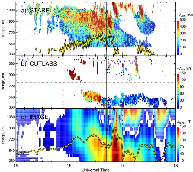
In this study we concentrate on a 3-h period between 15:00 and 18:00 UT on 27 March 2004, as this was the inter-val during which both the STARE and CUTLASS Finland radars observed coherent echoes at the radar cells near the EISCAT viewing area. This event provides a unique op-portunity for studying the E-region irregularity velocity as observed by VHF and HF radars in the context of informa-tion on the plasma moinforma-tions provided by an incoherent scatter radar. Figure 1 presents the range-time-intensity (RTI) plots of irregularity l-o-s velocity in (a) STARE Finland beam 4 and (b) CUTLASS Finland beam 5. Both velocities have been reversed so that the majority of the RTI cells are filled with the solid color (negative velocity), while cells filled with horizontal lines indicate that positive velocities were recorded. The STARE range cell closest to the EISCAT beam is shown by the dashed line (bin 24, 855 km) in panel (a). In panel (b), Doppler velocity at all frequencies is plotted for ranges >780 km (dotted line), while for closer ranges only the velocity in channel A (10 MHz) is considered.
Panel (c) shows the equivalent current component along the CUTLASS beam 5 direction. This has been estimated from the IMAGE magnetic perturbations as described be-low. The electrojet equivalent current vector was derived by
rotating the horizontal magnetic perturbation vector by 90◦
clockwise for each 1-min interval. This variation was com-puted for all stations in the IMAGE network for which data were available for this event and the results were
interpo-lated between 15◦–28◦E and 64◦–72◦N using a 0.5◦-step.
Panel (c) is a range-time-intensity plot along the CUTLASS beam 5 direction from the interpolated data. It provides a useful context for considering the variation of the E×B drift velocity component along the coherent radar beam direction since the latter can be approximated by the reversed com-ponent of the equivalent current assuming that the magnetic perturbations were mainly caused by the convection-related Hall electrojet currents in the absence of large density gradi-ents (Fukushima, 1976).
The STARE radar started to detect echoes at the farther ranges of 700–1100 km at ∼15:15 UT. The echoes became more abundant and formed a wide (∼500 km) band which started to move equatorward at around 16:00 UT, shortly be-fore the CUTLASS radar started to observe F-region echoes near EISCAT (above dotted line). In addition to F-region HF echoes, from 16:15 UT onwards, a ∼150-km-wide band of E-region HF echoes at 400–550 km was observed. At far-ther ranges, the F-region velocity changed its sign between 16:30 and 16:45 UT and in general agreed reasonably well with the equivalent current component shown in panel (c), which is not surprising since F-region velocity measured at a given direction should represent the E×B drift component (e.g. Davies et al., 1999).
The E×B drift velocity can be also inferred from the EISCAT tristatic measurements of ion velocity in the F-region since both plasma species should drift with E×B drift velocity at these heights. In Fig. 2 we show (a) the electron density measurements, (b) the magnitude and (c) the direction of the field-perpendicular ion velocity vector at 278, 115, and 110 km. The ion velocity data at 90, 95, and 105 km also collected in this experiment were not consid-ered in the present study, as these exhibited very large scat-ter and since the electron density and hence signal-to-noise ratio (SNR) were typically lower than those for higher alti-tudes (above 110 km), Fig. 2a. Figure 2 also shows (dotted black lines) the E×B vector (b) magnitude and (c) direction as inferred from the magnetic perturbations at Tromsø. The yellow dots in panels (b) and (c) are the F-region velocity magnitude and direction, respectively, determined from
fit-ting the cosine law curve VFcos(φ+φ0), where φ is the angle
between the radar beam and magnetic L-shell, to all HF ve-locities in the F-region as described in detail by Makarevitch et al. (2004a). The latter estimate represents the averaged (for all radar beams and ranges 780–1215 km) plasma con-vection in the F-region. Finally, the blue vertical bars repre-sent the azimuthal extent of the primary F-B instability cone
±θ0 inferred from the ion drift measurements at 278 km,
Vi2780 ∼=Ve0, and the ion acoustic speed Cs estimates from
EISCAT measurements of the ion and electron temperatures at 110 km: θ0=cos−1(Cs/Ve0), Cs=(kB(Ti+Te)/mi)1/2,
where kB=1.38·10−23J/K, mi=28.8·1.67·10−27kg.
The ion drift velocity magnitude at 278 km (Vi2780 ) slowly
increased during the first 1-h interval. At ∼16:00 UT both the electron density (at 110–120 km) and the electric field
magni-360 540 720 900 1080 Range, km 0 100 200 300 400 500 -VVHF, m/s
a) STARE
360 540 720 900 1080 Range, km 0 30 60 90 120 150 -VHF, m/sb) CUTLASS
360 540 720 900 1080 Range, km 10 40 70 100 130 160 Jcomp, nTc) IMAGE
15 16 17 18 Universal TimeFig. 1. Range-time-intensity plots for (a) VHF velocity in STARE Finland beam 4 (azimuth of -20.9◦), (b) HF velocity in CUTLASS Finland
beam 5 (azimuth of –20.1◦), and (c) IMAGE equivalent current vector component along the CUTLASS beam 5 direction, Jcomp. The colour
bar for each panel is shown on the right. Cells filled with solid colour (horizontal lines) correspond to negative (positive) velocity component. The dashed horizontal (thick yellow) lines in panels (a) and (c) indicate the range position of the EISCAT viewing area in the E-region (time variation of the STARE velocity and IMAGE current component at the EISCAT location in arbitrary units).
tude started to increase, although the latter showed some un-dulations. At ∼16:42 UT a large density enhancement, local-ized in time, was observed in the EISCAT data (Fig. 2a). We have indicated this time by the vertical line in Figs. 1 and 2. The ion velocities at 115 and 110 km generally exhibited sim-ilar trends to that at 278 km (Vi1150 ∼Vi2780 /2, Vi1100 ∼Vi2780 /4) except that they did not show undulations near 16:20 UT.
The ion velocity direction at 278 km was very close to –90◦
in azimuth (lowest horizontal dotted line in Fig. 2c, west-ward drift) for the first half of the interval under study, and
it was rotated by ∼30◦clockwise from the westward
direc-tion after ∼16:30 UT. Again, the ion velocity direcdirec-tions at 115 and 110 km followed that at 278 km, being rotated by
roughly 45◦and 90◦ anticlockwise, respectively. The other
two E×B drift estimates (from magnetic perturbations and
F-region HF data) showed similar trends to V278i0 except for the
interval near the density enhancement at ∼16:42 UT when the E×B drift estimate from magnetic perturbations was sig-nificantly different from V278i0 .
Large undulations in the EISCAT ion drifts (and hence in electric field) were only seen at 278 km. The magnetometer currents and CUTLASS velocities also did not show any
un-dulations comparable to those for Vi2780 , Fig. 2b. At 16:10–
16:20 UT the equivalent current (dotted line) was roughly constant with the CUTLASS velocity (yellow circles)
show-ing some increase, while Vi2780 dropped below Vi1150 . Electron
temperature measured with EISCAT at 110 km, that is often used as an indicator of the electric field strength, also was fairly constant (not shown). The above observations suggest
100 150 200 250 300 350 400 A lt , k m 0 1 2 3 4 5 Ne, 105 cm-3
a)
0 400 800 1200 1600 V el Io n P er p , m /s 110 km 115 km 278 kmb)
-180 -135 -90 -45 0 45 90 135 180 A z, d egc)
15 16 17 18 Universal TimeFig. 2. Panel (a) shows the EISCAT density data, Ne. Vertical line indicates the time of the density enhancement, 16:42 UT. Panels (b)
and (c) show the magnitude and direction (azimuth from the geographic north) of the field-perpendicular ion drift velocity inferred from the EISCAT tristatic measurements at several altitudes. The dotted black lines in panels (b) and (c) are the magnitude and azimuth of the
magnetic perturbation vector at Tromsø. The vector was rotated by 90◦anticlockwise to match the irregularity drift direction. The yellow
dots show the magnitude and azimuth of the F-region Doppler velocity inferred from the cosine fit to the CUTLASS velocity data in the
F-region. The blue vertical bars at each red dot in panel (c) show estimates for the primary F-B instability cone ±θ0.
16:20 UT might have been of instrumental origin. After 16:30 UT, variation in the ion drift magnitude is generally consistent with those in equivalent current and ion drifts at 110 and 115 km, Fig. 2b.
Finally, one should note that between 8 March and 2 De-cember 2004 the STARE Finland site computer had an accu-mulative timing error reaching 3 h 41 min 48 s at 07:31:10 UT
on 2 December 2004. To correct the timing error the
STARE Finland data was shifted by an appropriate
in-terval (∼17 min) assuming linear error accumulation. In
Figs. 1 and 2 the vertical line shows the time 16:42 UT when EISCAT started to observe enhanced densities at 110– 120 km. At approximately this time, the VHF velocity near EISCAT (thick yellow line in Fig. 1a) dropped drastically,
almost simultaneously with the drop in Jcompnear EISCAT
(yellow line in Fig. 1c) and the reversal in the F-region HF velocity (780–1215 km) although in the latter case it is dif-ficult to determine the reversal time accurately due to the patchiness of F-region HF echoes at 16:30–16:44 UT. This feature indicates that the timing error was accounted for with an accuracy of 1 min sufficient for the present study as it is fully consistent with numerous previous studies that showed that the electric field magnitude is depressed (enhanced) in-side (outin-side) the region of enhanced conductivity (e.g. del Pozo et al., 2002, and references therein). In our observa-tions, the VHF velocity (largely dependent upon the electric field) peaked at 16:33 and 16:46 UT with a sharp drop ob-served in between, that is at the time of the density enhance-ment apparent in the EISCAT data in Fig. 2a.
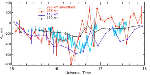
-800 -600 -400 -200 0 200 400 Vlos , m/s 278 km 278 km smoothed 115 km 110 km 15 16 17 18 Universal Time
Fig. 3. Comparison between the com-ponents resolved along the STARE beam 4 direction. The red, dark blue, and black lines show the EISCAT ion drift velocity component at 278, 115,
and 110 km, respectively. The light
blue line is the Doppler velocity mea-sured by the STARE radar in the radar cell corresponding to a range of 855 km. The vertical line shows the time of den-sity enhancement at 16:42 UT from Fig. 2a.
An examination of the equivalent current images obtained from the interpolated IMAGE data as described above (not presented here) shows that a crescent-shaped boundary be-tween currents of opposite sign (east- and westward elec-trojets) appeared in the region of interest after 16:30 UT. It then migrated equatorward reaching the Tromsø location at 16:45 UT shortly before it started to retreat poleward (16:47 UT). A similar pattern can be recognized in Fig. 1c
ex-cept for an additional enhancement in Jcompat farther ranges
(>950 km) at ∼16:42 UT, which is simply a consequence of
the fact that the projection direction (azimuth of –20.1◦) near
this particular moment of time happened to be almost tan-gential to the north-west pointing part of the crescent-shaped boundary. Absorption intensity images obtained in an anal-ogous fashion from the IRIS data show a sharp increase in absorption at 16:44 UT near EISCAT. These observations suggests that the density enhancement at ∼16:42 UT can be attributed to energetic particle precipitation near the convec-tion reversal boundary. One can assume then that the density enhancement was quite localized.
2.3 Relationship between irregularity velocity and ion and
electron motions in the E-region
In this report we concentrate on the comparison between the l-o-s velocity at VHF and the ion drift velocity compo-nent measured simultaneously by the STARE and EISCAT radars, respectively. The ion drift velocity component mea-sured in the F-region in this experimental configuration acts
as a proxy for the electron drift velocity in the E-region, Ve0.
Figure 3 presents a comparison between the STARE Dop-pler velocity in beam 4, range 855 km (light blue line, the same as reversed yellow line in Fig. 1a) and the component of the EISCAT ion drift velocity resolved along the direction of
the STARE beam 4 (azimuth –20.9◦) at 278 (red), 115 (dark
blue line with squares), and 110 km (black line with open circles). To reduce undulations in the ion drifts at 278 km, we also smoothed the EISCAT ion drift variations at 278 km
using a 3-point window and we show this variation in Fig. 3 by the dotted red line.
One can notice from Fig. 3 that before ∼16:30 UT the l-o-s velocity magnitude at VHF was typically smaller or close to the ion velocity component at 278 km (red, closed circles and dotted line). After 16:30 UT, however, the VHF veloc-ity was mostly larger in magnitude and/or opposite in sign
compared to Vi2780 . The ion velocity at 115 km (dark blue,
squares) was typically larger in magnitude than the VHF ve-locity except for one point near the vertical line. The ion velocity at 110 km (black, open circles), on the other hand, was either close to the VHF velocity (15:30–16:00) or some-what smaller (16:00–16:31 UT). Generally, the VHF veloc-ity was between the two E-region ion drift components, i.e.
Vi1100 .VVHF.Vi1150 , with the exception of the measurements
near 16:45 and 17:35 UT when it was larger and smaller, re-spectively, than either of the ion drift components.
Figure 3 shows that the time variation of the STARE Doppler velocity appears to be quite similar to the EISCAT-inferred electron motion component (ion drift at 278 km) be-fore 16:20 UT (this is more evident in the smoothed data). After 16:20 UT, however, these two variations differed sig-nificantly. Interestingly, for many measurements the VHF velocity was close to that of the ions at 110 km. The EISCAT F-region (E-region) ion velocity data in Fig. 2 had 5-min (10-min) resolution and ∼75-s integration period, while the STARE data was integrated over 20-s intervals, and in Fig. 3 we have smoothed the VHF velocity using a 3-point sliding window. Another approach is to post-integrate the STARE velocity using the appropriate intervals and to compare the irregularity and ion velocity directly by plotting them against one another. Figure 4 presents the results of this compari-son for the three altitudes of ion velocity measurement. The vertical bar for each point indicates the standard deviation associated with the averaging while the horizontal bars show the uncertainty associated with the ion velocity component (i.e. the same as the vertical bars in Fig. 3). As in Fig. 3 we
-600 -400 -200 0 200 Vion comp, m/s 15:42 15:52 16:02 16:11 16:21 16:31 16:41 16:51 17:22 17:32 c) 110 km -600 -400 -200 0 200 Vion comp, m/s 15:26 15:36 15:46 15:56 16:06 16:16 16:26 16:36 16:46 16:56 17:16 17:26 17:36 b) 115 km -600 -400 -200 0 200 Vion comp, m/s -600 -400 -200 0 200 V VHF los , m/s 15:40 15:45 15:50 15:55 16:00 16:05 16:10 16:15 16:20 16:25 16:30 16:35 16:40 16:45 16:50 16:55 17:20 17:25 17:30 17:35 a) 278 km smoothed
Fig. 4. Scatter plots of line-of-sight irregularity drift velocity measured by the STARE Finland radar in beam 4 and bin 24, VVHF los, against
the component of the EISCAT ion drift velocity resolved along the STARE beam 4 direction at (a) 278, (b) 115, and (c) 110 km. The time (interval centre) of measurements is indicated near each point.
used the smoothed EISCAT ion drift data at 278 km. In Fig. 4a, there is considerable scatter and measurements after 16:30 UT generally lie far from the ideal coincidence line. Moreover, three points are in the right-bottom quad-rant, that is their VHF Doppler velocity was of the opposite sign to that of the ions. At 115 km, Fig. 4b, the ion velocity component was larger than the VHF velocity (with the ex-ception of measurements near 16:46 UT). The VHF velocity was predominantly larger in magnitude or close to the ion velocity component at 110 km, Fig. 4c.
At both E-region altitudes, the VHF velocity exhibits some positive correlation with the ion drift component; the linear Pearson coefficient computed for the data presented in pan-els (b) and (c) are 0.45 and 0.49, respectively. The corre-lation coefficient is much smaller for the data in panel (a) (only 0.12). If one excludes from the correlation analysis the data near the density enhancement at 16:42 UT (at 16:46 and 16:41 UT in panels (b) and (c), respectively), the correlations at 115 and 110 km are quite substantial, viz. 0.80 and 0.79, respectively, whereas at 278 km it is only 0.44 even when as many as three points (at 16:35, 16:40, 16:45 UT) are ex-cluded. Correlation in panel (a) improves significantly if one includes only the points before 16:30 UT, viz. 0.61.
3 Discussion
In our observations, the electron drift velocity vector was
directed at an azimuth of 90◦–130◦W as inferred from the
EISCAT tristatic measurements of the ion drift velocity at 278 km, CUTLASS measurements of HF Doppler velocity in the F-region, and IMAGE magnetometer records, Fig. 2c.
Given the azimuth of the STARE beam 4 (20.9◦W), our
mea-surements of the Doppler velocity at VHF almost certainly refer to observations outside the instability cone. Indeed, our estimates of the azimuthal extent of the primary F-B
instabil-ity cone (blue bars centered on the electron velocinstabil-ity azimuth in Fig. 2c show that the instability cone might have reached
the azimuth range of interest (–20.9◦) for only one
measure-ment (∼16:20 UT). For all other measuremeasure-ments, it is rather unlikely that we observed the primary, in-cone irregularities. The experiment configuration employed in this study thus al-lows us to investigate irregularity velocity at large flow an-gles, outside the primary instability cone in the context of the electron and ion background motions.
Following previous STARE/EISCAT studies (e.g. Kofman and Nielsen, 1990; Kustov and Haldoupis, 1992; Koustov et al., 2002; Uspensky et al., 2003, 2004) we compared the
electron drift velocity component Ve0cos θ and the l-o-s
ve-locity measured with the VHF radar, VVHF los, Figs. 3 and
4a. Both line and scatter plots show that the l-o-s velocity at VHF represents the electron drift velocity component rather poorly.
In Fig. 4a, the majority of points were either close to or above the dashed line of ideal coincidence (for the same sign), that is their VHF velocity was smaller than the E×B drift velocity component. Koustov et al. (2002) have at-tributed significantly smaller STARE Finland velocity mag-nitudes, as compared to those of E×B drift velocity compo-nent, to the phase velocity attenuation with the aspect angle (Ogawa et al., 1980; Nielsen, 1986; Kustov et al., 1994) since the aspect angles near the EISCAT FoV for the STARE Fin-land observations have been estimated to be of the order of
–1◦. In addition, for a few points in Fig. 4a velocities were of
the opposite sign. This result is somewhat surprising as the velocity sense at VHF is expected to agree with that of the
E×B drift even if the magnitude is reduced due to the aspect
angle effects. Good agreement between the senses of veloc-ity measured directly with the STARE Finland radar and that inferred from the tristatic measurements with the EISCAT radar has also been shown experimentally (e.g. Kofman and Nielsen, 1990; Kustov and Haldoupis, 1992).
-800 -600 -400 -200 0 200 400 Vlos , m/s -5 Jcomp TRO -5 Jcomp KIL V HF fit comp VHF los 885 km VHF los 1020 km 15 16 17 18 Universal Time
Fig. 5. Comparison between the
E×B plasma drift components as
in-ferred from various techniques. The
green squares and black dots (yellow dots) represent the F-region velocity measured by the CUTLASS Finland radar in ranges 870–915 km and 1005– 1050 km, respectively (inferred from the cosine fitting to all F-region veloci-ties). The thin dark (heavy) blue line is the reversed equivalent current compo-nent at Tromsø (Kilpisj¨arvi).
In Fig. 2b, we showed that after ∼16:30 UT variation in the EISCAT ion drift magnitude at 278 km was similar to those at 110 and 115 km as well as to variation in the equivalent currents (with exception of measurements near 16:42 UT), which suggests that the EISCAT ion drift data
at 278 km was of reasonable quality. To provide
addi-tional evidence that the EISCAT ion drift data at 278 km is an appropriate proxy for the electron drift velocity in the E-region, in Fig. 5 we compare the EISCAT ion drift com-ponent at 278 km (both unsmoothed data shown by the red line and closed circles and 3-point smoothed data shown by the dotted line) with several other estimates of the E×B plasma drift component: (1) CUTLASS Doppler velocity measurements in beam 5, ranges 870–915 km (green squares, VHF los 885 km); (2) as for (1) but at ranges 1005–1050 km
(black dots, VHF los 1020 km); (3) the averaged fitted HF
ve-locity component in the F-region (yellow dots, VHF fit comp);
and the reversed equivalent current component (4) at Tromsø
(thin dark blue line, −Jcomp TRO) and (5) at Kilpisj¨arvi
(heavy blue line, −Jcomp KIL). The estimates (3) and (4) have
been obtained by simply projecting the two-dimensional vec-tors (yellow dots and dotted black lines, respectively) from Figs. 2b and c onto the STARE beam 4 direction. The es-timate (5) is analogous to (4) except that the magnetometer records at Kilpisj¨arvi were considered.
One should note that the location of the HF backscatter (in terms of slant range) is seldom known accurately. A stan-dard range-finding algorithm assumes a straight line prop-agation to a specific height (similar to a VHF coherent sys-tem), which for our observations gives a range of 885 km (for
EISCAT F-region FoV, 69.0◦N, 19.1◦E, 300 km).
Propaga-tion effects, such as ray bending, however, are significantly more important for HF observations, and generally cannot be ignored. Yeoman et al. (2001) showed that in their ob-servations at ∼19.5 MHz an uncertainty associated with the selection of the range gate in 1/2-hop propagation mode to Tromsø slightly exceeded the range gate length in Myopic
mode (15 km) and in Fig. 5 we considered three range gates 870, 885, and 900 km (870–915 km).
There were two intervals during which the CUTLASS Fin-land radar observed echoes in those ranges in beam 5 (green squares in Fig. 5): near 16 and 17 UT. For the first interval the HF velocity was of the same sign (being ∼20% smaller in magnitude) as the ion drift component while for the second interval it was of opposite sign (except for a few points near 17:15 UT). The fitted HF F-region velocity component (yel-low) utilizing measurements in all CUTLASS beams shows a somewhat different trend; it was negative and close to the HF l-o-s velocity at 885 km before 16:40 UT but more consistent with the ion drift component near 17:05 UT when both were positive.
The change in the F-region HF velocity sign and a velocity magnitude increase with slant range is obvious in Fig. 1b so that one can expect a better match between the EISCAT and CUTLASS measurements assuming some bending of the HF beam and hence larger slant ranges used for comparison. A
decrease of the equivalent current component Jcompwith
dis-tance from the radar can be also recognized in Fig. 1c and hence one can attempt to put both EISCAT and CUTLASS velocity measurements into the context of the equivalent cur-rent component near the EISCAT viewing area. Interestingly, HF l-o-s velocity at 885 km represents reasonably well the KIL current component (green squares are near the heavy blue line) after 17:00 UT, even though the straight line prop-agation distance between the radar site and the KIL magne-tometer (when its position is projected along the magnetic field line from 110 to 300 km) is only around 825 km. A similar comparison between the HF l-o-s velocity at 1020 km and the TRO current component also shows good agreement (straight line distance in this case is ∼920 km). The EISCAT
velocity component is between −Jcomp KILand −Jcomp TRO
(VHF los 885 kmand VHF los 1020 km) near 17:00 UT, which
in-dicates that HF echoes near EISCAT originated from some-where between these ranges, 885–1020 km. This uncertainty
in range is somewhat larger than that reported previously for a radar frequency of 19.5 MHz (Yeoman et al., 2001) but is consistent with more recent results of Yeoman et al. (2005) for lower frequencies for which the refraction effects are ex-pected to be more significant.
Ideally, to resolve the issue of the location of the HF echoes one needs to perform ray-tracing simulations using the electron density measurements along the HF radar beam. Unfortunately, no such measurements were available except for the Tromsø location, Fig. 2a, which is quite far from the region of interest (ranges 300–700 km) so that the results of any ray-tracing simulation would be applicable only if the horizontal density distribution were homogeneous. In an at-tempt to address the problem, a series of ray-tracing simula-tions using standard CUTLASS software based on the orig-inal code developed by Jones and Stephenson (1975) that implements Haselgrove (1963) method has been performed using the representative frequency of 10 MHz of channel A and EISCAT density profiles at 16:30–16:35, 16:38–16:40, 16:53–16:57, 17:03–17:06, and 17:13–17:16 UT, as well as the generic profile from the International Reference Iono-sphere (IRI) model (Bilitza, 2001) appropriate for the time (27 March 2004, 16:30 UT) and location of the measure-ments (to be consistent with other simulations in series the
Tromsø location, 69.0◦N, 19.1◦E, has been selected). The
results, however, indicate that the observed features, such as location of the E- and F-region backscatter and ground scat-ter are not reproduced adequately by any of the simulations, which most likely signifies that the lower portion of the iono-sphere was not quite homogeneous. This conclusion is to some extent supported by the Sodankyl¨a ionosonde observa-tions that show the E-region critical frequency f0E substan-tially smaller than the F-region critical frequencies f0F1 and f0F2, whereas EISCAT observed the E-region to be stronger and comparable to the F-region after 16:00 UT, Fig. 2a.
By taking everything into account, one can conclude that even though our best efforts to pinpoint the location of HF echoes was largely unsuccessful, the EISCAT data on the electron motions in the E-region, when placed in a context of CUTLASS and IMAGE measurements, appear to be of rea-sonable quality. Moreover, as we argue further in Sect. 3.1, several important features recognizable in the electron mo-tion data can be explained reasonably well and are consistent with previous studies. Furthermore, the interpretation below is also supported by the EISCAT data on the ion motions at 110 km that had an integration time almost twice as large.
The other issue that also needs to be discussed is the qual-ity of the STARE data. As we noted earlier, on a few occa-sions EISCAT and STARE velocities were of opposite sign. Uspensky et al. (2004) presented the STARE/EISCAT data showing that when the STARE SNR was very low (∼0 dB) the VHF velocity was of opposite sign to that of the E×B drift component (see their Fig. 2). This observation has been used later by Makarevitch et al. (2004b) in an attempt to ex-plain the STARE velocities measured near the poleward edge
of the VHF echo band that were not consistent with the di-rection of the plasma flow. In our observations, however, the power of STARE Finland echoes from near EISCAT (not shown here) was above 3 dB and typically between 8 and 30 dB. In this situation, we believe, other effect(s) could be important.
3.1 E-region irregularity velocity and ion motions
Moorcroft (1996) suggested that when E-region irregulari-ties propagate at large flow angles, i.e. nearly perpendicular to the plasma flow, they can move with a velocity that is sig-nificantly different from that of the electron motion compo-nent and close to that of the ions. This idea has been used to explain an asymmetry of the velocity variation with the
flow angle with respect to 90◦observed with the Homer UHF
radar.
According to the linear fluid theory of electrojet irregular-ities (e.g., Fejer and Kelley, 1980), the phase velocity at a
direction of wave propagation vector ˆk ≡k / k is given by
V = ˆ
k · Vd
1 + 9 + ˆk · Vi0, (1)
where Vd≡Ve0−Vi0, and 9 is a function of aspect angle
α, collision frequencies of ions and electrons with neutrals
(νi, νe) and ion and electron gyro frequencies (i, e):
9 = νeνi ei (cos2α + 2 e ν2 e sin2α). (2)
If the first term in Eq. (1) is small the phase velocity is deter-mined by the second term and hence would be representative
of the ion drift velocity component along ˆk and independent
of the aspect angle. This argument has been employed by Makarevitch et al. (2002) in order to explain an absence of velocity variation with slant range (and hence aspect angle) for certain directions as seen by the Prince George Super-DARN HF radar.
The above argument would be valid, however, only for the relatively small range of flow angle near perpendicularity to
Vdif perfect aspect angle conditions (α=0) are assumed.
Us-pensky et al. (2003) proposed that non-orthogonality of the scatter coupled with the ion motions could play a crucial role in modifying the phase velocity of E-region irregularities as it essentially widens the range of the flow angles for which the ion motions dominate since 9 grows rapidly with the as-pect angle α, Eq. (2), thus reducing the first term in Eq. (1). Even though in the Uspensky et al. (2003) observations the STARE Finland velocity and EISCAT convection component were of the same sign, it was argued that it is possible for them to have different sign (see their Figs. 8 and 9), an im-portant prediction in the context of the present study. Milan et al. (2004) argued that if the aspect angles are very large
(>3◦) the range widens even more, reaching small flow
that the l-o-s velocity sense can be opposite to that of the electron drift, which was supported by the observations with the CUTLASS Iceland radar at very short ranges (<400 km). Later Makarevitch et al. (2004a) have considered the varia-tion of the l-o-s velocity as measured by the CUTLASS Fin-land radar in the near FoV (range <1215 km) and demon-strated that velocities of opposite sign occur for a range of flow angles.
The principal difference between this and the previous studies is that in addition to ion velocity measurements in the F-region we also have information on the ion motions in the E-region. This was achieved by varying the EISCAT tristatic altitude in a manner similar to that reported by Davies et al. (1997) who used the ion velocities at 6 E- and 1 F-region heights to estimate the ion-neutral collision frequencies in the E-region. In the present study, we compare for the first time the E-region Doppler velocity measured with STARE and the ion drift velocity component from EISCAT measurements in order to test the previously proposed hypothesis concerning the importance of the ion motion.
The comparisons showed that the STARE velocity was roughly between the ion velocity components measured at 110 and 115 km, with exception of the measurements near the time when a large density enhancement was observed by EISCAT, 16:40–17:00 UT. Importantly, this was also near the interval when the STARE velocity exceeded the elec-tron velocity component, Fig. 3. Uspensky et al. (2003) have termed this feature “velocity overspeed” and attributed it to an increase in effective backscatter height. They argued that when observing a certain radar cell, the radar integrates over a range of E-region heights, and due to the height variation of the scattering cross-section the bulk of the backscatter power comes from a certain altitude, determined by altitude pro-files of the density and aspect angle. As the density profile changes with time so does the effective height of backscat-ter. In the E-region top side (115–120 km) the ion drifts are much greater than at the peak (105–110 km) and hence the ion motion contribution to the E-region irregularity velocity is greatly enhanced as well.
The VHF velocity was slightly smaller than the ion
ve-locity component at 110 km Vi1100 in the beginning of the
interval of interest but later on became larger and even
ap-proached and exceeded Vi1150 near the density enhancement at
16:42 UT, while being significantly different (larger in
mag-nitude and even of the opposite sign) from Ve0 at the same
time. These facts suggest that this variability could be re-lated to the changes in the electron density profile.
To test this idea we present the EISCAT electron density in the E-region, Fig. 6a, together with the velocity comparison
shown in Fig. 3. The maximum density height hmaxbetween
95 and 125 km is shown in panel (a) by the yellow dots. In cases when the electron density data was available on both
sides of the maximum the height hmaxwas taken as the
max-imum of the parabolic function fitted to the three points. Un-fortunately, the patchiness of the electron density data below
110 km does not allow us to estimate the effective
backscat-ter height heff for the entire duration of the event with 75-s
resolution. To overcome this by improving the data statis-tics and to match the resolution with that of STARE we have reanalyzed the EISCAT Tromsø data using 20-s integration intervals. These 20-s data sets were used further to estimate
the effective height heff using a technique described in
de-tail by Uspensky et al. (2003, 2004). The effective height estimates are shown by the red circles (20-s values) and hori-zontal lines (10-min averaged values shown if the number of points exceeded 5). The density profiles that had more than two missing data points (grey cells in Fig. 6) below 110 km or a missing data point just below 110 km were not considered. The remaining data gaps were filled by linear interpolation.
Figure 6 shows that before ∼16:00 UT the E-region elec-tron density was small and slightly increasing with altitude (the same feature is also evident in Fig. 2a). The STARE
velocity was slightly less or comparable to Vi1100 while the
effective height exhibited large scatter between 105–113 km but, on average, was below 111 km. After ∼16:00 UT the situation changes; a distinct E-region maximum appeared in
the density profiles around 112 km, heffwas generally above
110 km and, on average, around 113 km; the VHF velocity
was between Vi1100 and Vi1150 and agreed well with Ve0
(ex-cept for one measurement at 16:21 UT that might have been inside the instability cone, as we argued earlier). At 16:30–
16:40 UT, the spread in hmaxbecomes slightly larger and the
mean heffreaches an absolute maximum of 113 km, the VHF
velocity is larger than Ve0in magnitude and slightly less than
Vi1150 . In the next 10-min interval, during which a density
en-hancement occurred, heff showed strong fluctuations, while
hmaxwas typically above 125 km. At 16:50–17:00 UT, heff
was also variable peaking at ∼16:55 UT near the time when
EISCAT showed positive Ve0∼300 m/s. Between 17:15 and
17:35 UT, heff was decreasing towards the end of the
inter-val. The STARE velocity magnitude starts close to or slightly
above Vi1100 ending at somewhat lower values.
One can conclude that the timing of the changes in the relationship between irregularity and ion drift velocity (∼16:00, 16:30 UT) appears to be associated with the change in the density distribution and that the idea that an overspeed interval at 16:30–16:50 UT is associated with the uplifting of the E-region is to some extent supported by the electron density data as both maximum density and (less clearly) ef-fective backscatter height showed an increase at this time. The latter result thus supports previous findings by Uspen-sky et al. (2003). A new result with respect to irregular-ity and electron velocirregular-ity is that we report not just velocirregular-ity overspeed but also several cases of opposite velocity sign. Although envisaged earlier, it is instructive to establish ex-perimentally. One should note though that opposite signs were observed only in few cases so the result is perhaps not very conclusive. However, additional support for this point comes from a reanalysis of the EISCAT remote site data from 16:30 to 17:00 UT using a 20-s integration. We found that
105 110 115 120 125 130 Alt, km 0 1 2 3 4 5 Ne, 105 cm-3
a)
-800 -600 -400 -200 0 200 400 Vlos , m/s 278 km 278 km smoothed 115 km 110 kmb)
15 16 17 18 Universal TimeFig. 6. Panel (a) shows the EISCAT density data between 100–135 km at 20-s resolution. Colour scheme is indicated on the right. Grey cells represent missing data. The yellow (red) dots are the maximum density (effective backscatter) height between 95 and 125 km. The horizontal white lines are 10-min averaged effective heights. Panel (b) is the same as Fig. 3.
the tristatic velocity component consistently showed positive velocities of larger magnitudes than the uncertainty of the measurements near 16:45 and 16:55 UT, with larger spread and both negative and positive velocities near 16:35 UT. The latter result combined with the noted earlier observation that the CUTLASS velocities were also positive near 16:45 UT (albeit not exactly at the EISCAT location), makes it rather unlikely that the opposite signs were simply the result of the low data quality.
The other new result of the present study is that the VHF velocity was “limited” by the ion velocity components at 110 and 115 km. From Fig. 4, the VHF velocity magnitude was
above the ion drift component Vi1150 only once, namely at
16:46 UT, near the time of the density enhancement.
Simi-larly, it was well below Vi1100 only once, at 17:32 UT when
the effective height was below 110 km. If one assumes that the backscatter height varies slightly with time in a range 105–115 km (as both previous estimates by Uspensky et al.
(2003) and our own estimates of heff suggest), one can
in-terpret this observation as indicating that there will be
agree-ment between the VHF velocity and the ions drift component at a height within the 105 to 115 km range, with the height at which the agreement occurs depending upon the electron density profile.
According to this interpretation, agreement between the VHF velocity and the ion velocity component at 110 km be-fore 16:00 UT was observed simply because the bulk of the backscatter signal came from around this altitude, which
re-sulted in the observed closeness between VVHF losand Vi1100 .
The estimates of heff that we performed generally support
this notion as on average they were close to 110 km.
More-over, the VHF velocity was smaller than Vi1100 in
magni-tude during the intervals when heffwas below 111 km (e.g.,
15:50–16:00 UT or 17:30–17:40 UT). In general, the
varia-tion of the VHF velocity in Fig. 6b with respect to Vi1100 and
Vi1150 appears to be consistent with this variation of effective
height.
To emphasize this feature we present Fig. 7, which, for convenience shows the negative of the difference between the VHF velocity and the ion velocity component at 110 km
plot--4 -2 0 2 4 heff-h0, km -200 -100 0 100 200 300 400 -(V VHF los - V ion comp ), m/s 1542 1552 1602 1621 1631 1641 1651 1722 1732
a)
-2 0 2 4 heff-h0, km 1542 1552 1602 1611 1621 1631 1641 1651 1722 1732b)
Fig. 7. A difference between the STARE l-o-s velocity and the EISCAT ion drift component at 110 km (reversed) versus the
ef-fective backscatter height counted from h0=110 km and averaged
for (a) ∼10-min intervals centered at the time of the EISCAT mea-surements indicated near each point and (b) ∼2-min intervals of the EISCAT measurements.
ted against the effective height heffcounted from h0=110 km
and calculated using two methods described below. For
each EISCAT measurement with integration interval (t1, t2),
an appropriate interval over which to average the effective
height was determined as (t1−δ, t2+δ), where δ was taken as
(a) 4 min and (b) 0 s. The same interval (t1, t2)was used for
averaging the VHF velocity averaging in Figs. 4c and 7. The vertical bars in Fig. 7 represent standard deviations due to the averaging of VHF velocity (the same as the vertical bars in
Fig. 4c) plus uncertainties in Vi1100 (the same as the horizontal
bars in Fig. 4c) while the horizontal bars are standard devi-ations due to the averaging of effective height values from Fig. 6a. In this way, Fig. 7a features the effective height es-timates similar to those presented in Fig. 6a by white lines
(also ∼10-min intervals since t2−t1.150 s at h0=110 km,
but centered at the time of the EISCAT velocity measure-ments), whereas Fig. 7b shows averaged values using the intervals matched exactly with EISCAT and STARE veloc-ity post-integration intervals of Fig. 4c. Similar to Fig. 6a, Fig. 7a shows only those points for which the number of 20-s effective height values used in the averaging exceeded 5. De-spite the difference in approach, both diagrams show a sim-ilar pattern: a general increase of VHF velocity as a func-tion of effective height where both variables were counted from the reference level at a specific height of 110 km. The linear Pearson correlation coefficients between the variables in panels (a) and (b) are 0.73 and 0.76, respectively. The more thorough analysis of Fig. 7 thus confirms our conclu-sion based on Fig. 6, namely that the VHF velocity variation appears to be consistent with that of the effective backscatter height.
3.2 E-region irregularity velocity: relative importance of
electron and ion motions
The observations presented in this report suggest that the E-region irregularity velocity at large flow angles may represent
the ion velocity component at an altitude that varies between 108–114 km depending on the electron density profile. This result is different from those of the classical studies of the 1980s that demonstrated good agreement between irregular-ity and electron drift velocities in the E-region (Nielsen and Schlegel, 1983, 1985; Kofman and Nielsen, 1990) as well as from those of more recent studies that proposed that the ion drift motion should be taken into account (Uspensky et al., 2003, 2004; Makarevitch et al., 2004a).
It might be possible to reconcile these results by as-suming that both the ion drift velocity and its coupling to the irregularity phase velocity varies from one set of
ob-servations to another. In our observations near equinox
and during daytime, the ion drift velocity was relatively large; Vi1100 ∼Vi2780 /4, Vi1150 ∼Vi2780 /2, Fig. 2b. This re-sult is consistent with the estimate of the ion drift ve-locity based on the collision frequencies calculated us-ing the expressions given by Schunk and Nagy (1980) and the neutral densities taken from the MSISE-90 model run for the specific time and location of our
obser-vations (69.0◦N, 19.1◦E, 27 March 2004, 16:30 UT).
At 110 km, the ion-neutral collision frequency νin is
627 s−1and V110
i0 ∼i/νinVe0∼=0.29Ve0, where i∼=180 s
−1
is the ion gyrofrequency. At 115 km, νin=329 s−1 and
Vi1150 ∼=0.55Ve0. This result is also consistent with the
find-ings by Davies et al. (1997) who employed the ion drift velocity measurements at several heights to derive the
nor-malised collision frequency, νin/ i=((E/B)2/Vi20−1)1/2
to be of the order of 3.7 at 109 km, and hence obtained Vi1090 =(3.72+1)−1/2Ve0∼=0.26Ve0for similar conditions on
3 April 1992, 10:00–15:00 UT.
When considered in the context of the E-region irregular-ity velocirregular-ity the ion drifts are usually neglected (a fair approx-imation for observations at small flow and aspect angles) or estimated for a specific height using generic collision fre-quencies (e.g. Milan et al., 2004; Makarevitch et al., 2004a). One could argue that, depending on conditions (in particu-lar the soparticu-lar cycle period, season, and time of observations), the collision frequency can vary considerably and so can the ion drift velocity. For example, both our measurements and those of Davies et al. (1997) refer to the descending phase of the solar cycle. When solar activity is larger one can ex-pect larger collision frequencies and smaller ion drifts.
In-deed, the MSISE-90 model gives νin=671 s−1at 110 km for
27 March 2000, 16:30 UT, and a corresponding 7% reduction in the ion drift velocity, Vi1100 ∼=0.27Ve0. Similar estimates for
nighttime conditions (27 March 2000, 01:30 UT) give a fur-ther 15% reduction in the ion drift velocity as compared to the daytime conditions, Vi1100 ∼=0.23Ve0.
Another important factor can be the backscatter height, as we argued following the idea of Uspensky et al. (2003). Fi-nally, the “coupling function” 9 will differ for different sets of conditions as it depends upon the aspect angle (which ac-cording to Uspensky et al. (2003) depends upon the density
profile as does the backscatter height) and collision
frequen-cies. The electron collision frequency νe can also depend
indirectly on the electric field intensity due to electron scat-tering by the unstable F-B waves which effectively results
in enhanced “anomalous” collision frequencies νe∗ (Sudan,
1983; Robinson, 1986; Robinson and Honary, 1990). Thus, the results of the present study indicating that E-region
irreg-ularity velocity Vlos may represent the ion velocity, Vi0, at
large flow angles do not necessarily contradict the previous
findings that demonstrated either an agreement between Vlos
and Ve0(e.g. Kofman and Nielsen, 1990) or the agreement
between Vlosand a combination of Ve0and Vi0(e.g.
Uspen-sky et al., 2003).
Finally, during the first half of the interval under study the irregularity velocity exhibited much larger positive correla-tion with the electron drift component than that for the entire dataset (0.61 versus 0.12). This suggests that relative impor-tance of electron and ion drifts could differ even for one set of observations. Moreover, according to Eq. (1) one can expect the ion drift component to dominate over that of the elec-trons when the latter is small (when the flow angle is close
to 90◦). Interestingly enough, from Fig. 2c, the flow angles
were closer to 90◦after ∼16:30 UT when the electron drifts
were oriented at ∼110◦–120◦West of North while STARE
observations were performed at 20.9◦(also W of N), that is
exactly when the largest disagreements between irregularity and electron drift velocities were observed (including oppo-site signs). It is thus entirely feasible that if the ion drift “coupling function” is relatively small, variation in the flow angle would strongly affect the E-region irregularity velocity.
3.3 E-region irregularity generation at large flow and aspect
angles
In this study we concentrated on the phase velocity of E-region irregularities at large flow angles. The results psented suggest that the Doppler velocity measurements re-fer to observations at large aspect angles as well. In other words, we are dealing with irregularities propagating outside both the flow and aspect cones where the generation of irreg-ularities in the linear regime is prohibited. Nonlinear theories have been invoked in the past in order to explain plasma wave generation at large flow (Sudan et al., 1973) and aspect an-gles (e.g. Hamza and St-Maurice, 1995). Of special interest for this study is the recent work by Drexler and St.-Maurice (2005) who proposed that what appears as large aspect an-gle echoes in the HF radar data (Milan et al., 2004) can in fact be successfully interpreted using the nonlocal formula-tion of Drexler et al. (2002). Furthermore, Drexler and St.-Maurice (2005) have derived a formula for the phase velocity (rather than simply adopting the one from the linear theory) that only contains the ion drift term, thus providing a theo-retical basis for the interpretation used in Milan et al. (2004). Even though the nonlocal theory of Drexler et al. (2002) and Drexler and St.-Maurice (2005) strictly speaking applies only
to small flow angles, it provides additional insights as to why irregularities at large flow and aspect angles are observed at all as well as why their Doppler velocities appear to be close to that of the ion motion in the E-region.
If one assumes that the waves outside the flow angle in-stability cone are generated through the nonlinear cascade from the linearly unstable, small flow angle modes (Su-dan et al., 1973), then significant modification of the lin-ear phase velocity, Eq. (1), can occur. Based on 30-MHz imaging radar observations in conjunction with in situ elec-tric field measurements, Bahcivan et al. (2005) proposed that the phase velocity outside the flow angle cone is better de-scribed by the cosine component of the ion acoustic speed,
Cscos θ , than by the more often cited plasma drift
compo-nent, Vdcos θ . The ion acoustic speed was taken from the
empirical formula derived by Nielsen and Schlegel (1985) with the electric field magnitude as an input parameter. In our experiment the tristatic EISCAT system provided both electric field and temperature measurements allowing us to check whether the STARE l-o-s velocity was close to the
prediction based on the Cscos θ formula. The ion
acous-tic speed was calculated using the measured ion and elec-tron temperatures as in the previous calculation of flow an-gles shown in Fig. 2c. The results of this analysis showed that, indeed, for observations before ∼16:20 UT, the
agree-ment between Vlosand Cscos θ was better (than that between
Vlos and Vdcos θ ). After ∼16:20 UT, however, no
signifi-cant improvement was observed, as one would expect for an
“overspeed” case, i.e. Vlos>Vdcos θ , with substitution of Vd
by Cs<Vd generally making the agreement worse.
Varia-tion of the assumed height (we repeated Cs calculations for
110, 115, and 120 km) only resulted in very small changes
in the Cs component meaning that variation with altitude is
unlikely to account for large differences between Vlos and
Cscos θ when Vlos>Vdcos θ .
The present study provides an alternative view on the phase velocity at large flow angles to that proposed in Bahci-van et al. (2005) as we consider the ion drift rather than the ion acoustic speed to be important for Doppler observations
at large flow angles. It is not clear why exactly the Cscos θ
idea fails in the “overspeed” case nor whether these two ideas could be reconciled. To resolve these issues as well as the is-sue of the relative importance of the electron and ion motions in determining the E-region irregularity velocity one needs simultaneous and continuous data on the ion and electron motions and temperatures in the E-region. The present study employing the European incoherent scatter radar facility’s unique scanning capabilities to deduce the ion and electron velocities in a quasi-continuous fashion in conjunction with the STARE coherent VHF radar simultaneously measuring the E-region irregularity velocity is a first step in this direc-tion.
4 Conclusions
A comparison of the line-of-sight Doppler velocity measured by the STARE Finland VHF radar at large flow angles with the ion and electron drift velocity components inferred from the EISCAT tristatic observations of the ion motions in the E and F-regions, respectively, shows that the STARE ve-locity is close to the ion drift veve-locity component in the E-region (110–115 km), whereas correlation with the electron drift component is low at the largest flow angles and near sig-nificant enhancements in the E-region electron density. This suggests that the E-region irregularity velocity at large flow angles may represent the ion velocity component at an alti-tude determined by the plasma density altialti-tude profile.
The results of the first comparison between the irregular-ity and ion drift velocirregular-ity measurements in the E-region pre-sented in this study provide direct support to recent studies that found reasonable agreement between the measured and estimated velocity under the assumption that the ion drifts should be taken into account, but the results also suggest that the ion motion may play a greater role in the phase velocity of E-region irregularities than previously thought.
Acknowledgements. R. A. Makarevich gratefully acknowledges
funding from the Particle Physics and Astronomy Research Coun-cil, UK (research grant PPA/G/S/2001/00491). The STARE system is operated jointly by the Max Plank Institute for Aeronomie, Ger-many, and the Finnish Meteorological Institute, Finland, in coop-eration with SINTEF, University of Trondheim, Norway. We thank P. Janhunen of FMI for providing access to the STARE data on the FMI web site. EISCAT is an international association supported by Finland (SA), France (CNRS), Germany (MPG), Japan (NIPR), Norway (NFR), Sweden (NFR), and the UK (PPARC). The CUT-LASS radars are funded by PPARC, the FMI, and the Swedish Institute for Space Physics. The IMAGE magnetometer data are collected as a Finnish-German-Norwegian-Polish-Russian-Swedish project conducted by the Technical University of Braunschweig and FMI. The IRIS facility is funded by PPARC in collaboration with the Sodankyl¨a Geophysical Observatory.
Topical Editor M. Pinnock thanks D. Moorcroft and another ref-eree for their help in evaluating this paper.
References
Bahcivan, H., Hysell, D. L., Larsen, M. F., and Pfaff, R. F.: The 30 MHz imaging radar observations of auroral irregular-ities during the JOULE campaign, J. Geophys. Res., 110, doi:10.1029/2004JA010975, 2005.
Bilitza, D.: International Reference Ionosphere 2000, Radio Sci., 36, 261–275, 2001.
Browne, S., Hargreaves, J. K., and Honary, B.: An imaging riometer for ionospheric studies, Electronics and Communication, 7, 209– 217, 1995.
Buneman, O.: Excitation of field-aligned sound waves by electron streams, Phys. Rev. Lett., 10, 285–287, 1963.
Davies, J. A., Lester, M., and Robinson, T. R.: Deriving the nor-malised ion-neutral collision frequency from EISCAT observa-tions, Ann. Geophys., 15, 1557–1569, 1997,
http://www.ann-geophys.net/15/1557/1997/.
Davies, J. A., Lester, M., Milan, S. E., and Yeoman, T. K.: A com-parison of velocity measurements from the CUTLASS Finland radar and the EISCAT UHF system, Ann. Geophys., 17, 892– 902, 1999,
http://www.ann-geophys.net/17/892/1999/.
del Pozo, C. F., Foster, J. C., and St.-Maurice, J.-P.: Dual-mode E region plasma wave observations from Millstone Hill, J. Geo-phys. Res., 98, 6013–6032, 1993.
del Pozo, C. F., Williams, P. J. S., Gazey, N. J., Smith, P. N., Honary, F., and Kosch, M. J.: Multi-instrument observations of the dy-namics of auroral arcs: a case study, J. Atmos. Sol. Terr. Phys., 64, 1601–1616, 2002.
Drexler, J. and St.-Maurice, J.-P.: A possible origin for large aspect angle HAIR echoes seen by SuperDARN radars in the E-region, Ann. Geophys., 23, 767–772, 2005,
http://www.ann-geophys.net/23/767/2005/.
Drexler, J., St.-Maurice, J.-P., Chen, D., and Moorcroft, D. R.: New insights from a nonlocal generalization of the Farley-Buneman instability problem at high latitudes, Ann. Geophys., 20, 2003– 2025, 2002,
http://www.ann-geophys.net/20/2003/2002/.
Farley, D. T.: A plasma instability resulting in field-aligned irreg-ularities in the ionosphere, J. Geophys. Res., 68, 6083–6093, 1963.
Fejer, B. G. and Kelley, M. C.: Ionospheric irregularities, Geophys. Rev., 18, 401–454, 1980.
Fukushima, N.: Generalized theorem for no ground magnetic ef-fect of vertical currents connected with Pedersen currents in the uniform-conductivity ionsophere, Rep. Ionos. Space Res. Jpn., 30, 35–40, 1976.
Greenwald, R. A., Weiss, W., Nielsen, E., and Thomson, N. R.: STARE: A new radar auroral backscatter in Northern Scandi-navia, Radio Sci., 13, 1021–1029, 1978.
Greenwald, R. A., Baker, K. B., Dudeney, J. R., Pinnock, M., Jones, T. B., Thomas, E. C., Villain, J.-P., Cerisier, J.-C., Senior, C., Hanuise, C., Hunsuker, R. D., Sofko, G., Koehler, J., Nielsen, E., Pellinen, R., Walker, A. D. M., Sato, N., and Yamagishi, H.: DARN/SuperDARN: A global view of the dynamics of high-latitude convection, Space Sci. Rev., 71, 763–796, 1995. Haldoupis, C.: A review on radio studies of auroral E region
iono-spheric irregularities, Ann. Geophys., 7, 239–258, 1989, http://www.ann-geophys.net/7/239/1989/.
Hamza, A. and St-Maurice, J.-P.: Large aspect angles in auroral E region echoes: A self-consistent turbulent fluid theory, J. Geo-phys. Res., 100, 5723–5732, 1995.
Haselgrove, J.: The Hamiltonian ray path equations, J. Atmos. Terr. Phys., 25, 397–399, 1963.
Jayachandran, P. T., St.-Maurice, J.-P., MacDougall, J. W., and Moorcroft, D. R.: HF detection of slow long-lived E region plasma structures, J. Geophys. Res., 105, 2425–2442, 2000. Jones, R. M. and Stephenson, J. J.: A versatile three dimensional
ray tracing computer program for radio waves in the ionosphere, OT Report 75-76, US Dep. of Comm., Washington, D.C., USA, 1975.
Keskinen, M. J., Sudan, R. N., and Ferch, R. L.: Temporal and spatial power spectrum studies of numerical simulations of type 2 gradient drift irregularities in the equatorial electrojet, J. Geo-phys. Res., 84, 1419–1430, 1979.