HAL Id: hal-02428439
https://hal.archives-ouvertes.fr/hal-02428439
Submitted on 3 Jul 2020
HAL is a multi-disciplinary open access
archive for the deposit and dissemination of
sci-entific research documents, whether they are
pub-lished or not. The documents may come from
teaching and research institutions in France or
abroad, or from public or private research centers.
L’archive ouverte pluridisciplinaire HAL, est
destinée au dépôt et à la diffusion de documents
scientifiques de niveau recherche, publiés ou non,
émanant des établissements d’enseignement et de
recherche français ou étrangers, des laboratoires
publics ou privés.
A global model of the magnetorotational instability in
proto-neutron stars
Alexis Reboul-Salze, Jérôme Guilet, Raphaël Raynaud, Matteo Bugli
To cite this version:
Alexis Reboul-Salze, Jérôme Guilet, Raphaël Raynaud, Matteo Bugli. A global model of the
magne-torotational instability in proto-neutron stars. Journées de la SF2A, Société Francaise d’Astronomie
et d’Astrophysique, May 2019, Nice, France. �hal-02428439�
A GLOBAL MODEL OF THE MAGNETOROTATIONAL INSTABILITY IN
PROTO-NEUTRON STARS
A. Reboul-Salze
1, J. Guilet
1, R. Raynaud
1and M. Bugli
1Abstract. The magnetorotational instability (MRI) is a promising mechanism to amplify the magnetic field in fast-rotating proto-neutron stars. Many local studies have shown that the magnetic field could be amplified on small scales. However, the efficiency of the MRI at generating a large-scale field similar to the dipolar magnetic field of magnetars (1014− 1015 G) is still unknown. We used a three dimensional
pseudo-spectral code to develop an idealized global model of the MRI in a proto-neutron star. We show that a dipole field strength consistent with the values of magnetar field intensity can be generated by the MRI, even though it is lower than the small-scale magnetic field. Overall, our results support the ability of the MRI to form magnetar-like dipolar magnetic fields.
Keywords: magnetars, supernovae, magnetohydrodynamics (MHD), instabilities, methods: numerical
1 Introduction
Magnetars are a class of neutron stars which stand out by their emission in gamma-rays or X-rays (Kaspi & Beloborodov 2017, and references therein). A few objects are detected by their pulsar-like radio emission. The observations of these emissions measure the spin-down of the neutron stars. Under the assumption of magnetic braking, a surface dipolar magnetic field of 1014-1015G can be inferred from the spin-down of magnetars.
Several scenarios have been invoked to explain the origin of magnetar magnetic field. It may stem from the field of the progenitor amplified by magnetic flux conservation. However this scenario tends to fall short for the strongest magnetic fields. The other scenarios are the in-situ magnetic field amplification by a turbulent dynamo in the proto-neutron star (PNS), either by a convective dynamo (Thompson & Duncan 1993; Raynaud et al. 2020) or the magnetorotational instability (MRI, Akiyama et al. 2003; Obergaulinger et al. 2009).
The MRI was first discovered in the context of accretion disks by Balbus & Hawley (1991) and its properties have been well studied in this context. However, the physical conditions in proto-neutron stars differ from accre-tion disks. A strong differential rotaaccre-tion resulting from the core-collapse of the progenitor to a PNS was found in simulations (Akiyama et al. 2003; Ott et al. 2006). The MRI can develop in this strong differential rotation zone. This instability has been mainly studied in the local approximation analytically or by using “shearing box” simulations representing a part of the PNS. For weak magnetic fields (1012-1013G), the wavelength of the MRI
is indeed short and difficult to resolve in a global model. The first local simulations in the context of supernovae have shown that an efficient amplification of the magnetic field happens at the small scales (Obergaulinger et al. 2009; Rembiasz et al. 2016). Due to the high density inside the PNS, neutrinos are trapped inside it and their radiation induces a high viscosity, which can limit the growth of the MRI if the initial magnetic field is too low (Guilet et al. 2015).
The impact of the spherical geometry of the full PNS on the MRI turbulence and the ability of the MRI to generate a large-scale field, similar to the observed magnetic field of magnetars, is much less known. Mösta et al. (2015) performed the first simulations describing a quarter of the PNS with a high enough resolution to resolve the MRI wavelength. The model was, however, started with a strong progenitor magnetic dipole and therefore does not represent the scenario in which the MRI generates the magnetar magnetic field.
In this paper, we study the global properties of the MRI in spherical geometry using a different approach, in which the physical setup is reduced to its minimum physical ingredients. This has the advantage to pro-vide a useful reference for our physical understanding. Furthermore, this approach drastically reduces the computational cost and makes the exploration of the parameter space possible.
1 AIM, CEA, CNRS, Université Paris-Saclay, Université Paris Diderot, Sorbonne Paris Cité, F-91191 Gif-sur-Yvette, France
c
516 SF2A 2019
2 Numerical setup
The simulations performed in this article are designed to represent a fast rotating PNS of M = 1.3M and a
radius of ro = 25 km. In order to simplify the setup, we use the incompressible approximation. Furthermore,
we assume that neutrinos are in the diffusive regime and their effect is described by a viscosity ν = 7.03 × 1011 cm2s−1. We choose the physical parameters of the simulations to represent a fast rotating PNS model similar to the study of Guilet et al. (2015). Our model has a density ρ0 = 4 × 10¹³ g cm−3. The characteristic
angular frequency Ω = 103 s−1 matches the mean rotation rate. We use a cylindrical rotation profile with a
central part that rotates like a solid body and an outer part that follows a power law of r−q, with q = 1.25. The resistivity η is expected to be many orders of magnitude smaller than the viscosity, but numerical simulations for realistic values of the resistivity requires a too high resolution. In our study, we use a magnetic Prandtl number Pm= ν/η = 16. The initial magnetic field strength is varied from B0= 6.31 × 10¹⁴G to B0= 3.36 × 10¹⁵G.
Spherical harmonics and radial Fourier modes are randomly initialised for a wavelength interval [Lmin, Lmax].
This intense and small-scale magnetic field can be interpreted as the result of the first amplification described in local models. In order to solve the incompressible MHD equations with explicit diffusivities, we used the pseudo-spectral code MagIC (Wicht 2002; Schaeffer 2013). All the simulaitons presented in this paper were performed using a grid resolution of (nr, nθ, nφ) = (257, 512, 1024). For boundary conditions, we assume non-penetrating
radial velocity at top and bottom (vr= 0). For the inner boundary, we use standard no-slip boundary (~v = 0)
whereas for the outer boundary we force vφ to match the initial rotation profile at all times. For the magnetic
field, we compare several conditions: pseudo-vaccuum (normal field), perfect conductor (tangential field), or insulating (matching a potential field outside the domain).
3 A fiducial run
Let us first describe the results from a representative simulation. We initialised the magnetic field as decribed in section 2 with the parameters B0= 8.83×10¹⁴G, [Lmin, Lmax] = [0.3−0.5]. We also applied insulating boundary
conditions for the magnetic field. The left panel of figure 1 shows the temporal evolution of volume-averaged poloidal, toroidal magnetic energies and turbulent kinetic energy. The axisymmetric differential rotation is not included in the turbulent kinetic energy. After approximately 500 milliseconds, we obtain a quasi-stationary state, where the magnetic field intensity is B = 2.5 × 10¹⁵ G. The main contribution is from the toroidal magnetic energy that is 4-5 times stronger than the poloidal magnetic energy. The total magnetic energy is also more than ten times stronger than the turbulent kinetic energy.
Toroidal magnetic field
Poloidal magnetic field
Turbulent kinetic field
Total magnetic field
Total dipole field
Axial dipole field
Fig. 1. Left: Temporal evolution of the magnetic and turbulent kinetic energy for B0 = 8.83 × 10¹⁴ G, [Lmin, Lmax] =
[0.3 − 0.5]. The purple and green lines are the toroidal and poloidal contributions of the magnetic energy, while the dash-dotted orange line is the kinetic turbulent energy (axisymmetric toroidal contribution is removed). Right: Temporal evolution of the total magnetic energy and dipolar energy.
To describe more accurately the complex geometry of the magnetic field, it is essential to look at the state of the simulation at a given time. The figure 2 shows a representative snapshot of the quasi-stationary state with a 3D rendering of the magnetic field amplitude (left panel) and the toroidal magnetic field in the meridional plane (right panel). The winding of the magnetic field by the shear is clearly seen in the equatorial plane. The largest visible scales in this snapshot are due to the winding. On the meridional cuts, the magnetic field is more
Fig. 2. Left: 3D snapshot of the amplitude of the total magnetic field. The colors represent the magnetic field amplitude from (weak) blue to strong (red). Right: Azimuthal magnetic field Bφin the meridional plane for φ = 0.
chaotic at small scale. The meridional slice (right panel) shows that the radial coherence of the initial magnetic field has vanished in favor of small turbulent structures. At the poles, the magnetic field is not very intense due to the solid body rotation for this cylindrical radius. The velocity field presents similar characteristics. The MRI-driven turbulence is present for a cylindrical radius larger than r ≈ 9.4 km.
Since the magnetar timing parameters only constrain the dipole field strength, we focus in more details on this specific mode. The right panel of figure 1 shows the time evolution of the total magnetic energy (black line), the axial (green line) and total dipole (blue line). The dipole is not the dominant mode in the simulation as its energy is approximately 1000 times smaller than the total magnetic energy. But its strength is equal to Bdip = 1.25 × 10¹⁴ and could reach 5 × 10¹⁴ G with the conservation of the magnetic flux once the PNS
cools down and contracts to r = 12 km. Therefore we obtain a self-sustained MRI dynamo with a dipole field intensity that matches current observations.
4 Parameter study
The impact of initial conditions and boundary conditions on the magnetic field in the quasi-stationary state needs to be assessed. A small-scale magnetic field may initially lead to a lower intensity because a too incoherent magnetic field may first decay faster than it grows via the MRI in local models (Bhat et al. 2017). However, once the dynamics reaches a quasi-stationary state, we may expect that it is independent of the initial conditions as observed in local models. The initial magnetic field here is controlled by two parameters: the allowed length interval for the Fourier and spherical harmonic modes [Lmin, Lmax] and the initial magnetic field amplitude B0.
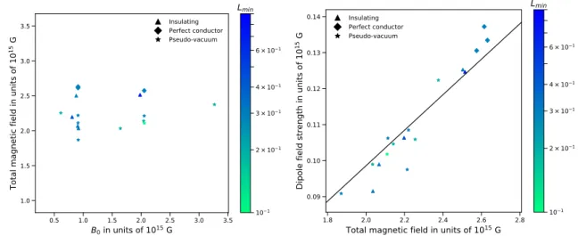
The left panel of figure 3 shows the time-averaged and volume-averaged magnetic field strength as a function of the initial magnetic field strength B0. No clear impact of the initial conditions can be seen in the figure.
Many models have similar magnetic field strength and different boundary conditions or initial conditions. The magnetic strength varies from 1.8 × 10¹⁵ G to 2.7 × 10¹⁵ G, which is a 15% difference around the median. A
part of this variation can be explained by the stochasticity of the MRI driven dynamos as often found in MHD turbulence. The magnetic field is slightly stronger in the case of perfect conductor boundary conditions but models with other boundaries still occupy the entire intensity range. It shows that the initial conditions and boundary conditions have a small impact on the final quasi-stationary state.
The global properties of the different models are found to be similar. This implies that the small scales and the turbulence do not depend on the boundary conditions. However, the differences should also be checked for the large scales that are constrained by the observations. The right panel of figure 3 shows the dipole amplitude as a function of the total magnetic field strength. It is clear from this figure that the dipole amplitude scales linearly with the total magnetic field. The results on the dipole mode are, thus, robust to both initial and boundary conditions. Our parameter study support the idea that the MRI is a robust mechanism to generate a magnetic field from differential rotation, which could lead to the formation of a magnetar.
518 SF2A 2019 0.5 1.0 1.5 2.0 2.5 3.0 3.5 B0 in units of 1015 G 1.0 1.5 2.0 2.5 3.0 3.5 To ta l m ag ne tic fi eld in u nit s o f 1 0 15 G Insulating Perfect conductor Pseudo-vacuum 101 2 × 101 3 × 101 4 × 101 6 × 101 Lmin 1.8 2.0 2.2 2.4 2.6 2.8
Total magnetic field in units of 1015 G
0.09 0.10 0.11 0.12 0.13 0.14 Di po le fie ld str en gt h in un its of 1 0 15 G Insulating Perfect conductor Pseudo-vacuum 101 2 × 101 3 × 101 4 × 101 6 × 101 Lmin
Fig. 3. Left: Total magnetic field strength as a function of the initial magnetic field strength. Right: Dipole field strength as a function of the total magnetic field strength. The equation of the linear fit is y = 0.0493x. The color indicates the smallest scale Lminof the initial magnetic field. The shape of the points represents the magnetic boundary
conditions between perfect conductor (diamond), insulating (triangle) and pseudo-vacuum (star).
5 Conclusion
Using numerical simulations of an idealized global model of a proto-neutron star, we have investigated the generation of a large-scale magnetic field by the MRI. In our simulations, the MRI leads to a quasi-stationary state with the following characteristics: it has a strong turbulent magnetic field of Btot ≥ 1015 G and a
non-dominant dipole component Bdip ≥ 1014 G that lies within the lower end of the intensity range for the dipole
of magnetars. Such a strong magnetic field could impact the dynamics of the core-collapse and launch jet-driven explosions, even though the complex geometry of our magnetic field may reduce the efficiency of the magnetorotational launching mechanism (Bugli et al. 2020).
We showed that the magnetic field amplification and dipole generation by the MRI is a robust mechanism with respect to the initial conditions and magnetic boundary conditions. Indeed, the turbulent energies and angular momentum transport in the quasi-stationary state does not depend on the initial magnetic field. The dipole strength scales linearly with the total magnetic field strength. These results support the ability of the MRI to generate a strong dipole and may explain the formation of magnetars.
Finally, we know that some limitations may have a quantitative impact on the results of our model (e.g. strength of the magnetic field and its dipolar component, etc.). For instance, taking into account buoyancy effects and the background density gradient may change these results (Guilet & Müller 2015). Our next step will be to implement a realistic interior model using the anelastic approximation to investigate the influence of these limitations.
This research was supported by the European Research Council through the ERC starting grant MagBURST No. 715368. The computations were performed on the CINES supercomputer occigen (applications A0030410317 and A0050410317).
References
Akiyama, S., Wheeler, J. C., Meier, D. L., & Lichtenstadt, I. 2003, ApJ, 584, 954 Balbus, S. A. & Hawley, J. F. 1991, ApJ, 376, 214
Bhat, P., Ebrahimi, F., Blackman, E. G., & Subramanian, K. 2017, MNRAS, 472, 2569
Bugli, M., Guilet, J., Obergaulinger, M., Cerdá-Durán, P., & Aloy, M. A. 2020, MNRAS, 492, 58 Guilet, J. & Müller, E. 2015, MNRAS, 450, 2153
Guilet, J., Müller, E., & Janka, H.-T. 2015, MNRAS, 447, 3992 Kaspi, V. M. & Beloborodov, A. M. 2017, ARA&A, 55, 261 Mösta, P., Ott, C. D., Radice, D., et al. 2015, Nature, 528, 376
Ott, C. D., Burrows, A., Thompson, T. A., Livne, E., & Walder, R. 2006, ASTROPHYS. J. SUPPL. S., 164, 130 Raynaud, R., Guilet, J., Janka, H.-T., & Gastine, T. 2020, Science Advances, in press
Rembiasz, T., Obergaulinger, M., Cerdá-Durán, P., Müller, E., & Aloy, M. A. 2016, MNRAS, 456, 3782 Schaeffer, N. 2013, Geochemistry, Geophysics, Geosystems, 14, 751
Thompson, C. & Duncan, R. C. 1993, ApJ, 408, 194
![Fig. 1. Left: Temporal evolution of the magnetic and turbulent kinetic energy for B 0 = 8.83 × 10 14 G, [L min , L max ] = [0.3 −0.5]](https://thumb-eu.123doks.com/thumbv2/123doknet/14767253.589058/3.892.170.754.745.942/fig-left-temporal-evolution-magnetic-turbulent-kinetic-energy.webp)