Radiative transfer in multifractal clouds

HAL Id: hal-02025315

https://hal.uca.fr/hal-02025315

Submitted on 19 Mar 2021

HAL is a multi-disciplinary open access

archive for the deposit and dissemination of

sci-entific research documents, whether they are

pub-lished or not. The documents may come from

teaching and research institutions in France or

abroad, or from public or private research centers.

L’archive ouverte pluridisciplinaire HAL, est

destinée au dépôt et à la diffusion de documents

scientifiques de niveau recherche, publiés ou non,

émanant des établissements d’enseignement et de

recherche français ou étrangers, des laboratoires

publics ou privés.

Radiative transfer in multifractal clouds

R. Borde, Harumi Isaka

To cite this version:

R. Borde, Harumi Isaka. Radiative transfer in multifractal clouds. Journal of Geophysical Research,

American Geophysical Union, 1996. �hal-02025315�

JOURNAL OF GEOPHYSICAL RESEARCH, VOL. 101, NO. D23, PAGES 29,461-29,478, DECEMBER 27, 1996

Radiative

transfer

in multifractal

clouds

R6gis Borde and Harumi Isaka

Laboratoire de M6t6orologie Physique, Universit6 Blaise Pascal, Aubi•re, France

Abstract. We studied effects of the cloud inhomogeneity in subcloud scale on the reflectance, transmittance, and absorptance of two-dimensional, inhomogeneous clouds. We generated the inhomogeneous clouds as multifractal clouds with a lognormal multiplicative process. For such clouds, the information codimension C• is a measure of the cloud inhomogeneity. Radiative transfer through the multifractal clouds was computed with a discrete angle radiative transfer model. The average reflectance, transmittance, and absorptance of multifractal clouds with a given codimension were estimated as averages of 200 realizations. They were computed for different sets of the C• parameter, cloud total optical thickness, and asymmetry factor of cloud scatterers. An effective optical thickness of inhomogeneous clouds was defined empirically in the framework of a homogeneous, plane parallel cloud model. Consequently, computation of radiative flux in an

inhomogeneous cloud could be transformed into that of an equivalent homogeneous, plane parallel cloud. For a two-dimensional, inhomogeneous, absorbing cloud we found that an inhomogeneous cloud absorbs generally less energy than its homogeneous counterpart. An exception was found for inhomogeneous clouds characterized by a small information codimension, a large cloud optical thickness, and a large single-scattering albedo and for which absorptance is much larger than for their homogeneous counterpart. However, this increase was less than 5% of the homogeneous cloud absorptance. The use of the effective optical thickness also enabled us to treat an inhomogeneous absorbing cloud as an equivalent homogeneous absorbing cloud and to estimate the radiative flux of the equivalent homogeneous cloud as an approximation to the one in the inhomogeneous

cloud. We found no immediate need to conceive of a direct effect of the cloud

inhomogeneity on the single-scattering albedo, as far as we considered this treatment as a first-order approximation. We discussed the use of the effective optical thickness in two- stream radiative approximations. We also compared our results with those based on the independent pixel approximation.

1. Introduction

The effect of clouds on the radiation budget of the atmo- sphere is one of the fundamental issues for the study and

modeling of the climate. Radiative fluxes and absorption in the

clouds are frequently estimated in the framework of a uniform plane-parallel cloud and two-stream approximation [Coakley

and Chylek, 1975; Joseph et al., 1976; Stephens, 1978a, b; Mea-

dor and Weaver, 1980; Zdunkowski et al., 1980]. Recent studies

tend to show that the absorption of solar energy by clouds might be much larger than that expected from typical cloud radiative transfer models and call into question the real effect

of clouds on the atmosphere and Earth radiation budgets [Ra-

manathan et al., 1995; Cess et al., 1995].

The area-averaged albedo and transmission of broken cloud

fields have been investigated by many physicists [Aida, 1977;

Wendling, 1977; Schmetz, 1984; Welch and Wielicky, 1984; Jo-

seph and Kagan, 1988; Br•on, 1992; Barker, 1992]. In these

studies the broken cloud fields were generated by distributing

randomly or regularly clouds with simple geometrical shapes

and different sizes over a limited area. The clouds were also

assumed to have uniform microphysical characteristics. The

cloud shapes and distributions assumed in these studies were

quite idealized, when compared with those in real broken Copyright 1996 by the American Geophysical Union.

Paper number 96JD02200.

0148-0227/96/96JD-02200509.00

cloud fields. The radiative transfer through the broken cloud fields still remains one of the major issues in the theory of

atmospheric radiation.

Clouds, even apparently homogeneous stratiform clouds, ex-

hibit a highly inhomogeneous distribution of liquid or ice water

content at subcloud scale induced by turbulent air motion [Duroure and Guillemet, 1990; Brenguier, 1990]. The inverse convection induced by radiative cooling at the cloud top also plays an important role in generating inhomogeneity in ex- tended stratiform clouds. Such inhomogeneity in the micro-

physical properties may have significant influence on the radi-

ative properties of the clouds. Effects of such cloud

inhomogeneity have been discussed in relation to the unex-

plained cloud absorption-albedo anomaly [Davis et al., 1990;

Stephens and Tsay, 1990]. Effects of the cloud inhomogeneity

were studied for various kinds of fluctuations of the optical thickness: sinusoidal variations [Weinman and Swarztrauber,

1968], stochastic variations [Mikhaylov, 1982], or experimen-

tally observed variations of liquid water content [Welch and

Wielicki, 1984; Cahalan et al., 1994a, b]. However, there still is

no well-established theoretical framework to deal with the

radiative transfer in inhomogeneous media [Fouquart et al.,

1990].

The classical approach of this problem was often limited to

study relationships between microphysical and optical proper-

ties of the inhomogeneous clouds at a "characteristic" scale,

though the interaction between clouds and radiation occurs

29,462 BORDE AND ISAKA: RADIATIVE TRANSFER IN MULTIFRACTAL CLOUDS

over a wide range of scales [Lovejoy and Schertzer, 1992]. Love-

joy et al. [1990], Gabriel et al. [1990], and Davis et al. [1990] studied recently the radiative transfer in fractal clouds with conservative scatterers, by using a discrete angle radiative

transfer (DART) model with a four- or six-stream scattering

phase function. They showed that the albedo and transmission

through fractal clouds could be expressed as a function of the

total cloud optical thickness and cloud fractal dimension.

Barker [1992] and Evans and Stephens [1993] also discussed the

radiative transfer in inhomogeneous clouds. Barker [1992] sug-

gested a possible adaptation of homogeneous, plane parallel

radiative transfer model to capture effects of the cloud inho-

mogeneities. More recently, Cahalan et al. [1994a, b] proposed

an effective optical thickness of inhomogeneous cloud based

on the independent pixel approximation (IPA).

The purpose of the present study is also to examine the

possibility to transform the radiative transfer in the inhomo-

geneous clouds into the usual framework of uniform plane

parallel clouds. Such a transformation, if possible, should be of

practical importance for the radiative flux computation in cli-

mate modeling as well as for the retrieval of cloud parameters from spaceborne radiometer data. We simulated radiative transfer by using the DART model in horizontally and verti- cally multifractal clouds generated with a lognormal multipli-

cative process [Monin and Yaglom, 1975a, b] in vertical plane.

Fluctuations of the water content in a multifractal cloud

generated by a pure multiplicative process are more intermit-

tent than those in natural clouds. In spite of this unnaturalness,

we adopted the lognormal multiplicative process because the

cloud inhomogeneity can be completely characterized by the

information codimension C•. No such parameter has been

defined yet to describe completely the intermittency of natural

clouds. This uniqueness of the inhomogeneity parameter

should make it easier to analyze simulations and parameterize

the intermittency effect on the cloud radiative properties. Since

the present study mainly aims to show a feasibility of such

approach, the precise representation of the cloud inhomoge-

neity may be expected not to be essential to its results.

We have defined an effective optical thickness of an inho-

mogeneous cloud and shown how this parameter varies with

cloud characteristics: the C • parameter, total optical thickness

of the cloud, and asymmetry factor of the scattering phase

function. The study was extended to the case of nonconserva-

tive scatterers to investigate effects of cloud inhomogeneity on

the radiative properties of absorbing clouds. We evaluated how

the absorptance of inhomogeneous clouds varies as a function

of the information codimension C •, total optical thickness to,

and single scattering albedo to o. Then, we examined how the

effective optical thickness could be integrated into the frame-

work of the plane parallel homogeneous cloud and that of

typical two-stream approximations. Finally, we compared our

evaluation of effective optical thickness with those derived

from the IPA.

2. Generation of Multifractal Clouds

To investigate effects of the cloud inhomogeneity on the

cloud radiative properties, we need not only to generate an

inhomogeneous cloud, but also to estimate statistical parame-

ters that provide a complete quantitative description of the

cloud inhomogeneity. This is not an easy task because we still

do not know what is meant by a complete quantitative descrip-

tion of the cloud inhomogeneity or what aspect of the inho-

mogeneity has effective influence on the cloud radiative prop-

erties.

Many physicists have recently had recourse to the fractal and

multifractal analysis of real clouds and cloud fields to investi-

gate their scaling and autosimilarity properties [Lovejoy, 1982;

Duroure and Guillemet, 1990; Joseph and Cahalan, 1990; Mar-

shak et al., 1994; Tessier et al., 1993]. The grounds for this

recourse are that the degree of inhomogeneities can be char-

acterized with only a few parameters, but these parameters,

once estimated, can be used to generate other fields with the

same multifractal characteristics [Schertzer and Lovejoy, 1991;

Davis et al., 1993; Marshak et al., 1994].

A multifractal medium can be easily generated with multi-

plicative cascade process [Monin and Yaglom, 1975a, b; Parisi

and Frisch, 1985]; this process is also called "weighted cur-

dling" by Mandelbrot [1983]. The lognormal process used here

follows that formalized by Yaglom as a model of eddy break-

down and described by Monin and Yaglom [1975a, b]. One

starts with an initial homogeneous field (in our case a homo-

geneous square) with a given total mass Mo of scatterers. One

subdivides this initial square into four subsquares, and after-

wards, repeats the same operation to each newly formed subs-

quare. After n steps of subdividing, the initial square is divided

into 2 2n subsquares.

At each

step

of subdividing,

the mass

in a

subsquare is distributed over four newly created subsquares

according to a prefixed rule of cascade. Mass in a cell after n

steps is given by

mn = mn-lOtn--- M0o•1o•2 ' ' ß O•n, (1)

where Mo, m n_ • and m n are the mass in the initial square,

n - lth and n th step cells, respectively; a i is a multiplicative

factor at thejth subdividing step. Different rules can be defined

and adopted to select the multiplicative factor a at each sub-

dividing step. The mass distribution at large scale modulates

multiplicatively the mass at smaller scale, which assures the

self-similarity and scale invariance of the field and creates a

hierarchy of singularities. Stochastic variables In a•,..., In a n

are assumed to have a normal distributions with a mean r• and a variance/•2. Hence the mean and the variance of the variable

In m n can be expressed as

thn = In (mn) = In (M0) + A (x) + n r•

(2)

2 = A l(X) + n t• 2

O' n

where A(x) and A •(x) represent the effect of the first few

coefficients ai.

In this way, an initial homogeneous distribution of the mass

Mo is transformed into an inhomogeneous distribution over

the same area. The mean of the variable m n is independent of

the observation scale Xn (= L o/2n), where L o is the size of

the initial square. Consequently, the mean r• is related to the

variance

/.•2

of the Gaussian

generator

by r/ = -/•2/2 [Monin

and Yaglom, 1975a]. The qth order statistical moment of m n

may be written as

2

mqn

= Mg

exp

{3q(q

- 1)(o'

n + A1)

} • M•(Xn/Lo)

-1/2q(q-1)V2

(3)

This expression is formally identical with the qth-order sta-

tistical moment of a multifractal field ex(x) at an observation

scale X [Schertzer and Lovejoy, 1987]:

BORDE AND ISAKA: RADIATIVE TRANSFER IN MULTIFRACTAL CLOUDS 29,463

where the function K(q) is a convex function with predeter-

mined values K(0) = K(1) = 0. A generalized dimension Dq

is defined by

K(q)

Dq=D (5)

q-1

and the information codimension C1 is defined by

C1

= D - D1

= dq

(6)

where D is the topological dimension of the space [Hentschel

and Procaccia, 1983]. The information codimension C• repre-

sents a measure of intermittency of the field. As C• increases

from 0 for a homogeneous medium to D, the total mass of the

scatterer tends to be distributed over fewer and fewer points; for C• = D, all the mass is found at a randomly positioned single point. A case with C1 > D is called "degenerated," meaning that every realization is empty and, now and then, a realization occurs with a huge peak [Davis e! al., 1993]. By

equating the exponent of (3) with the function K(q), we have

•

/z2.

X(q)

- q)

(7)

The multifractal field generated by a lognormal multiplicative

process with r/= -/•2/2 has an information codimension C 1 = /•2/2. In other words, a multifractal field with a given C • can

be generated by choosing the variance of the lognormal distri-

bution /•2 __ -2r/ = 2C•. Such a multifractal field is a

nonlacunary and dense fractal according to Mandelbrot's [1983] terminology.

The one-dimensional (l-D) spatial correlation of the lognor-

mal field can be expressed in the form

r ) -

+ r) -

(8)

where r and L are the observation and external scales, respec-

tively [Monin and Yaglom, 1975a, b]. Generally, the correlation

decreases

with the distance

r, but for too rapid

decay

(/•2 > 1),

the correlation becomes basically a "quasi-6 correlation" [Mar-

shaket al., 1994].

The Fourier spectrum S(K) corresponding to this autocor-

relation function is given by

S(K) • K '+•:: K-•

(9)

where K is the wave number. Since the variance/•2 is positive,

the spectrum slope cannot be steeper than -1 as C• ap-

proaches 0. Therefore fluctuation spectra generated by a pure

multiplicative cascade process are flatter than those of liquid

water content in real clouds, for which spectral slopes between

-3/2 and -3 were often reported [King e! al., 1981; Barker, 1992]. Marshak et al. [1994] tried to remedy this limitation in

spectral slope, by introducing a second multifractal parameter

H•, which represents a "nonstationary" state of fluctuations.

Shortcomings of the lognormal process were also discussed by

Frisch [1996].

In spite of this unnatural feature of pure multiplicative cas-

cade fields, we still used two-dimensional multifractal clouds

generated with lognormal multiplicative process. We did so

because we have investigated the impact of cloud inhomoge-

neity on the radiative transfer as a function of other cloud

optical parameters (total cloud optical thickness, asymmetry

factor and single-scattering albedo of the scatterers) and we

had to keep the number of parameters used to generate the

LOcal

optical

thickness

8

C1 = 0.05

128

z

LOcal

optical

thickness

,

(a)

C1 = 0.5

(b)

128

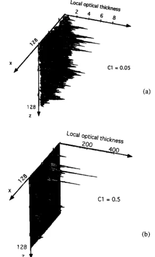
Figure 1. Multifractal fields of the scatterer mass generated

with a multiplicative lognormal cascade process and different

information codimensions' (a) C• = 0.05 and (b) C• = 0.5.

Both fields have the same total mass of the scatterer.

inhomogeneous clouds as small as possible. The lognormal

multiplicative process generates a "one-parameter-controlled"

inhomogeneous medium, in which both the probability distri-

bution and the spatial correlation of fluctuations are defined by

the information codimension C•. As was mentioned above,

this made the search for an empirical relationship between radiative properties and inhomogeneity parameter of the

clouds significantly easier.

Like other random cascade models, the lognormal process is

nonconservative, [Frisch, 1996], so after we generated a mul-

tifractal cloud, we recomputed the total mass of the generated cloud by adding the mass of all the elementary cells. When this recomputed mass differed from the initial one, we corrected the mass in each elementary cell by multiplying it with a cor-

rection factor and conserved the initial mass of the cloud. To

illustrate how the cloud inhomogeneity varies with C•, we

reproduced examples of two-dimensional (2-D, x-z) multifrac-

tal clouds generated with the C • parameter respectively of 0.05

and 0.5 (Figures la and lb). As C• increases from 0.05 to 0.5,

the mass becomes distributed over fewer cells, and the local

density of these cells becomes much higher.

3. Discrete Angle Radiative Transfer Model

To compute the radiative transfer in a 2-D multifractal cloud such as those presented above, we have two options: a Monte

29,464 BORDE AND ISAKA: RADIATIVE TRANSFER IN MULTIFRACTAL CLOUDS

Carlo code or a discrete angle radiative transfer code in which

light scatters only in a limited number of angular directions.

The DART model with a four-stream (six streams for 3-D

case) scattering phase function was previously used to compute

radiative transfer in fractal media [Lovejoy et al., 1990; Gabriel

et al., 1990; Davis et al., 1990; Gierens, 1993]. Although the DART model implies overhead sun and a limited number of

scattering directions, it nevertheless allows the effects of cloud

inhomogeneity to be studied in some detail. It also requires

much less computing time. Hence we adopted the DART model in this study.

By discretizing the radiative transfer equation, the DART

equation can be expressed for a four-stream scattering func-

tion in the following form:

I(x, u) - I(x - uSx, u) - I(x, u)Sr + to0tru,uI(x, u)Sr

+ • to0tru,vI(x-

vax, v)ar

(10)

where I(x, u) is the intensity in the direction of propagation u

at a position x. The quantity to o represents the single-scattering

albedo of the cloud scatterer, and the local optical thickness of

a cell is given by 8r = trp(x)Sx, where tr, p(x), and 8x are the

extinction coefficient, scatterer density, and size of the elemen-

tary cell, respectively. The quantity tru, v represents the fraction

of the energy scattered from the direction v into the direction

u. Equation (10) is obtained by discretizing the direct light in

the implicit mode and discretizing the side scattering and re-

flection in the explicit mode. This semi-implicit equation differs

from the explicit mode used by Lovejoy et al. [1990], Gabriel et

al. [1990], and Davis et al. [1990]. Local transmittance and

reflectance are expressed for the explicit and semi-implicit

discretizations in the following forms:

Explicit mode

I(x + u 8x, u)

t = I(x, u) = 1 - 8 r(1 - Oootru,u)

I(x-uSx, -u)

r =

I(x, -u)

- 8rtootru,_u

Semi-implicit mode

I(x, u) 1

t •- '--

I(x- uSx, u) 1 + 8r(1 -

I(x, -u) 8rto0tr,,_u

I(x + uSx, u) 1 + 8r(1 -

(11a)

(11b)

The energy side-scattered or absorbed by a cell is expressed

respectively by •J T OO O O'u,u ñ 1 + at(1- tOoO'.,.) at(1 - too) 1 + at(1 - tOoO'u,.) (11c) S -- a --

In the explicit mode, we have t --> -

oo, while t -• 0 and r

This means that in the case of a cell with a very high local

optical thickness the explicit mode would not provide correct

local values of transmittance and reflectance [Gierens, 1993].

The asymmetry factor is equal to g = tr•,u - tr•,_•. For the conservative scattering, we verify tr,, + 2tru,,ñ + tr,,_, =

1 and r + 2s -• 1 as 8r -• oo in the semi-implicit mode. Davis

et al. [1990] showed that the transmitted and reflected energy

computed by means of a DART model agreed with those

obtained with a Monte Carlo code and validated the DART

approach in computing radiative fluxes in inhomogeneous

clouds.

The cloud top was illuminated with a uniform normalized flux of incident energy. Equation (10) was solved numerically

by a relaxation method. Iterations were stopped when the differ-

ence between sums of incoming (I+(0) = 1 and I_(ro) = O)

and outgoing (I_ (0) and I + (to) ) fluxes was less than 0.1% for

a conservative scattering and when the transmitted, reflected,

and absorbed energies at every pixel in the domain did not change more than 0.1% during an iteration for absorbing

clouds. Clouds were simulated in a domain of 128 x 128

square cells, each cell having a local value of cloud optical

thickness 8rii. We adopted a cyclic lateral condition. The semi-

implicit scheme can also provide exact two-stream solutions for

a homogeneous cloud with the conservative scattering and

cyclic lateral boundary conditions.

4. Definitions of the Average Transmittance,

Reflectance and Optical Thickness in

Inhomogeneous Clouds

Figures 2a and 2b illustrate the simulated transmission of

light in a homogeneous cloud and an inhomogeneous cloud,

respectively. The transmission of light through the inhomoge-

neous cloud varies from point to point as a function of the

spatial distribution of scatterers, while the transmission in the

homogeneous cloud changes regularly with the distance from

the cloud top. Light penetrates deeply into the less dense part

of the cloud and hardly through much denser parts. Evaluating

the influence of cloud inhomogeneity corresponds to evaluat-

ing the nonlinear contribution of this larger transmission of

light through optically thinner parts in the cloud.

The optical thickness in a homogeneous cloud varies pro-

portionally as a function of the geometrical depth, while such

a proportionality cannot be valid for an inhomogeneous cloud.

Therefore in dealing with an inhomogeneous cloud, we need to

define an average optical thickness in a way compatible with

both homogeneous and inhomogeneous clouds. We defined

the average optical thickness at the ith level as the vertical sum

from the first to the ith layer of the horizontally averaged local

optical thickness:

l

Ti --- Z ( •j Tlj)J'

j=l

(12a)

where ( )i designates

the average

over n cells (Srli, l =

1, "', n) in the j th layer. According to this definition, the

total average optical thickness of the inhomogeneous cloud

can be kept identical with that of the homogeneous cloud. The

average optical thickness in the inhomogeneous cloud does not

vary linearly with the geometrical depth as in the homogeneous

cloud. The total transmittance T i at the i th layer is the hori-

zontal sum of transmitted energy Tli through n cells in the i th

layer:

ri •- Z rli.

(12b)

BORDE AND ISAKA: RADIATIVE TRANSFER IN MULTIFRACTAL CLOUDS 29,465

The horizontal average and sum are taken over the largest

horizontal scale of fluctuations of scatterers concentration in the cloud. This scale is equal to the side length L 0 of the cloud

domain in the present study.

When one generates inhomogeneous clouds with a given

mass of scatterers and a given C 1, there are an infinite number

of inhomogeneous clouds that are apparently different. This

also arises a need to estimate the average radiative behavior of

inhomogeneous clouds as an set average over all the possible

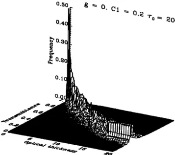
realizations. A two-dimensional distribution of frequency of

occurrence was estimated as a function of transmittance and

optical thickness for a set of 200 clouds (Figure 3). Each cloud

has the same set of parameters: a total optical thickness of

r 0 = 20, an asymmetry factor g = 0, a geometrical depth of

128Az (where Az is the thickness of each layer), and C1 =

0.2.

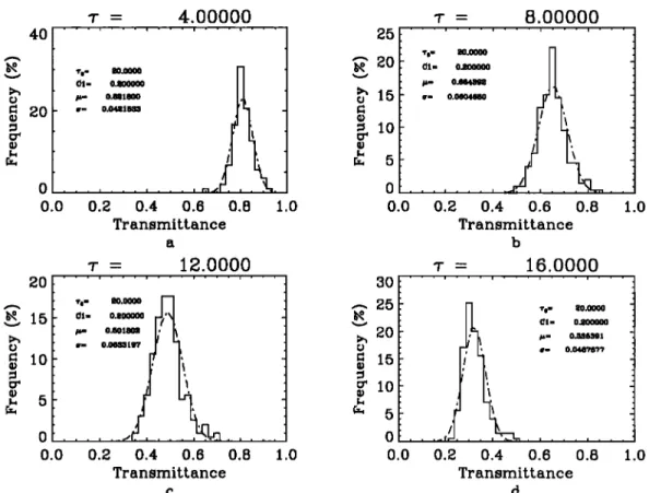
We reproduced histograms of the transmittance for four

different values of the average optical thickness, r = 4, 8, 12,

and 16 (Figure 4). The mean and standard deviation are

ø'1•ø g • 0 0.1( 0.0{

ß

C

l • 0.2

.ro•

20

Homogeneous cloud

Heterogeneous

cloud

Figure 3. Joint distribution of frequency of occurrence as a

function of the transmittance and optical thickness. The fre-

quency of occurrence was estimated from 199 realizations of

the inhomogeneous cloud with a total optical thickness of 20

and an information codimension of 0.2.

0.822 _+ 0.042, 0.664 _+ 0.060, 0.501 + 0.063, and 0.335 _+ 0.047,

respectively. The skewness is slightly negative for r = 4 and

positive for other values of r, and the tail of the distribution

becomes more important for large r. We tested the Gaussianity

of these distributions by applying X 2 and Kolmogorov-Smirnov

tests to the cumulative frequency of occurrence. The tests

showed that all the distributions could be considered as normal

distribution at a significant level of 10%.

We computed the transmittance in other inhomogeneous

clouds with the same mass of scatterers (r o = 20), but with

different C• parameters. The standard deviation increases with

C1 (Table 1), because the mass distribution of a multifractal

cloud with a large C 1 has fewer and more intermittent singu-

larities and consequently changes considerably from one real-

ization to another.

0

0 50 100

b Horizontal extension

Figure 2. Intensity of transmitted light through (a) a homo-

geneous cloud and (b) an inhomogeneous cloud as computed

with the DART model. Both the clouds have same average

total optical thickness of 20. The inhomogeneous cloud is gen-

erated with an information codimension of 0.3.

5. Radiative Fluxes Through Multifractal

Clouds in Conservative Scattering

5.1. Variation of the Transmittance With C•

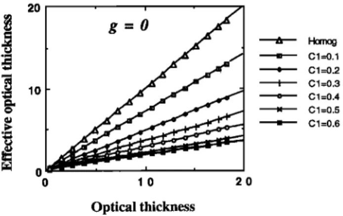
In Figure 5 we plotted the average transmittance as a func-

tion of the average optical thickness for inhomogeneous clouds

with the same total optical thickness r 0 = 20 and different

values of C1. The line labeled "homog" presents the transmit-

tance with the optical depth in the homogeneous cloud, which

is a linear function with a slope of -1/(2 + r0). For r < 3 the

transmittance through the inhomogeneous clouds decreases

with the optical thickness in the same way for all C1. In the

range r > 3 the transmittance through inhomogeneous clouds

decreases almost linearly as a function of the average optical

thickness for any value of C 1. As the optical thickness becomes

large, more photons can interact with the scatterers, and the

multiple scattering becomes more important. Hence the trans-

mission of light is more dependent on the spatial inhomoge- neity of the scatterers.

29,466 BORDE AND ISAKA: RADIATIVE TRANSFER IN MULTIFRACTAL CLOUDS 40 • 20 20 'r = 4.00000 ß . . , . . . , ß •. . , . . . , ß . . 01- •- o.•1•oo •- o.o4•1•5 . . . , . . . ! . . . ! rrl ..( 0.0 0.2 0.4 0.6 0.8 1.0 Transmittance ß = 12.0000 ß . . , . . . , . . . , . . . , ß . .

•=

0.0•51•7

f 1

Figure 4. Histograms of the transmittance at four different average optical thickness (z = 2, 4, 8, and 16).

The histograms are established from 199 realizations of the inhomogeneous cloud with a total optical

thickness of 20 and an information codimension of 0.2. The estimated means and standard deviations of these

histograms are 0.822 +_ 0.042, 0.664 +_ 0.060, 0.501 +_ 0.063, and 0.335 +_ 0.047 for z = 2, 4, 8, and 16,

respectively; the normal distributions with these means and standard deviations are plotted.

with C1 because more light is transmitted through the part of

the cloud with smaller local optical thickness. Figure 5 con-

firms that an inhomogeneous cloud transmits a greater amount

of energy than a homogeneous one. Since the scattering is

supposed to be conservative, an inhomogeneous cloud has a

smaller albedo than a homogeneous one.

5.2. Definition of an Effective Optical Thickness

These inhomogeneity effects may be taken into account by

defining an "effective OlStical parameter" as a function of C •. A

basic idea is to define this effective optical parameter so that

Table 1. Variation of the Standard Deviation of the

Transmittance at Four Optical Thickness in

Inhomogeneous Clouds

Standard Deviation of Transmittance

C 1 T = 4 z = 8 z = 12 z- 16 0.1 0.022 0.033 0.033 0.023 0.2 0.042 0.060 0.063 0.047 0.3 0.049 0.073 0.076 0.060 0.4 0.059 0.081 0.089 0.079 0.5 0.066 0.097 0.109 0.100 0.6 0.063 0.089 0.102 0.098

The inhomogeneous clouds are generated for a given total optical

thickness of 20 with different information codimensions C 1. The stan- dard deviation are estimated as an ensemble average over 199 realiza-

tions.

the radiative transfer in inhomogeneous clouds might be

treated in the classical framework of a plane parallel homoge-

neous cloud. Such a definition should take into account not

only the C 1 parameter but also the asymmetry factor g of the

1.0 0.8 0.6 0,4 0.2 g=O 0,0 0 10 20 Optical thickness • C1=0.1 • C1=0.2 I C 1 =0.3 • c1=0.4 -,4 c1=0.5 -- c 1 =0.6

Figure 5. Variation of the transmittance in inhomogeneous

clouds as a function of the average optical thickness. The

transmittance is computed as an ensemble average over 200

realizations of the inhomogeneous cloud with the same cloud

characteristics. The inhomogeneous clouds have the same total

optical thickness of 20, but they are generated for different

information codimensions (C1 = 0, 0.1, 0.2, 0.3, 0.4, 0.5,

and 0.6); the cloud with C1 = 0 represents a homogeneous

BORDE AND ISAKA: RADIATIVE TRANSFER IN MULTIFRACTAL CLOUDS 29,467

scatterers and the cloud total optical thickness r o. For simplic-

ity, we will first define this effective optical thickness as a function of only C1 and afterward consider the effects of the other parameters.

An effective optical thickness r' of an inhomogeneous cloud

is defined as the optical thickness of an "equivalent" homoge-

neous cloud that would have the same transmittance as that of

the inhomogeneous cloud. This is shown schematically in Fig-

ure 6. T(r, r o, C1) represents the transmittance for an optical

thickness of r, through a cloud with a total optical thickness to,

and C1. For conservative scattering, the global transmittance

of a homogeneous cloud with a total optical thickness r o is

given by the two-stream approximation solution: T(r o, r o,

C• = 0) = 2/[2 + (1 - 9)ro] [Meador and Weaver, 1980].

The curve labeled "2 streams" represents this relation.

An equivalent homogeneous cloud is a homogeneous cloud

that has the same total transmittance as that of the inhomo-

geneous cloud. The total optical thickness r/• of the equivalent

homogeneous cloud is given by the relation

2

T(r;,

r;, C•: 0): 2 + (1 - 9)r;

where T(rb, rb, C1 = 0) and T(%, %, C1 = 0.5) designate

the global transmittance of the equivalent homogeneous cloud

with a total optical thickness of rD and that of the inhomoge-

neous cloud with a total optical thickness of r o and a C1 of 0.5,

respectively. The total optical thickness of the equivalent ho-

mogeneous cloud is the "effective" total optical thickness of

the inhomogeneous cloud. The straight line labeled "equiv

homog" represents the transmittance in a homogeneous

cloud that is equivalent to the inhomogeneous cloud labeled

1.0 0.8 0.2 0.0 0 ß i , •:' 10 •: 20 Optical thickness 1 =0.5 streams Equiv homog

Figure 6. Schematic representation of the definition of an

effective optical thickness r' of an inhomogeneous cloud. The

"C1 = 0.5" curve represents the transmittance versus optical

thickness relation for an inhomogeneous cloud with a total

optical thickness of 20 and an information codimension of 0.5.

The "homog" line represents the transmittance versus optical

thickness relation for a homogeneous cloud with the same

optical thickness of 20. The "equiv.homog" line represents the

transmittance versus optical thickness relation of an "equiva-

lent" homogeneous cloud that has the same global transmit-

tance as the inhomogeneous cloud. The effective optical thick-

ness of the inhomogeneous cloud is defined by taking the

optical thickness on this line corresponding to the transmit-

tance of the inhomogeneous cloud. The "2 streams" curve

represents the global transmittance versus total optical thick-

ness relation of a homogeneous cloud obtained under the

two-stream approximation. 2O 10 o o lO 20 • C1=0.1 - C 1 =0.2 t C 1 =0.3 .--o--.-- C1=0.4 ;.; C1=0.5 -- C 1 =0.6 Optical thickness

Figure 7. Variation of the effective optical thickness as a

function of the optical thickness for the same inhomogeneous

clouds as in Figure 5. The inhomogeneous clouds have the

same total optical thickness of 20, but they are generated for

different information codimensions (C• = 0, 0.1, 0.2, 0.3,

0.4, 0.5, and 0.6); the cloud with C1 = 0 represents a homo-

geneous cloud.

"C1 = 0.5". The slope of the "equiv.homog" line is given by

2/[2 + (1 - 9)r•]. The "effective" optical thickness of the

"C1 = 0.5" inhomogeneous cloud is estimated by taking the

correspondence:

' c: 0): = 0 5)

TO, 1 ß ß

This equation means the transmittance T(r', r;, C1 = 0) for

an optical thickness r' in an equivalent homogeneous cloud

(C] - 0) is identical with that T(r, %, C1 : 0.5) for an

optical thickness r in an inhomogeneous cloud (C• = 0.5).

We applied this transformation of the average optical thick-

ness r into the equivalent optical thickness r' to all the curves in

Figure 5. The effective optical thickness r' is plotted as a function

of the average optical thickness r for various C ] (Figure 7); the

total optical thickness of the clouds is kept constant ro = 20.

For large optical thickness (r > 3), r' exhibits a linear variation

as a function of r. A priori, these curves should be subject to the following conditions:

lim r' = 0 (15a) •'--->0 lim r': r (15b) C•0

lim drJ = 2+ (1-9)r0

where r, r', and C1 are the usual optical thickness expressed by

equation (12a) the effective optical thickness, and the infor-

mation codimension of the inhomogeneous cloud, respectively.

The first condition is a trivial condition expressing that when

the usual optical thickness is small, the corresponding equiva-

lent optical thickness is also small. The second condition is that

a homogeneous cloud is its own equivalent homogeneous cloud. The third condition results directly from the ratio be- tween the slope of T(r', r•, C1 = 0) and that of T(r, r o, C1 -- 0). We have already shown above that in the uppermost

layer of an inhomogeneous cloud (r < 3) the inhomogeneity

29,468 BORDE AND ISAKA: RADIATIVE TRANSFER IN MULT!FRACTAL CLOUDS

• T(z < 3, Zo, C1 -• 0). In spite of this fact, the corre-

sponding effective optical thickness should depend on the de-

gree of cloud inhomogeneity because the effective optical

thickness is defined in the framework of the two-stream ap-

proximation and the total cloud optical thickness has to be

transformed in the equivalent total cloud optical thickness. The fourth condition implies that for large optical thickness

the effective optical thickness varies linearly with the average

optical thickness of the inhomogeneous clouds and that the

slope is function of the degree of inhomogeneity C 1. Accord-

ingly, we assumed that the semiempirical expression of the

equivalent optical thickness z' can be written in the following

form:

'r

'= {B(C1,

T0)C

1 q-

F(C1)'r}

1 - exp -•-•11 '

(16)

where A is a constant, B (C 1, Zo) is a function of C 1 and %,

and F (C 1) is a function of C 1 only. From (15c), we can derive the relation between A and B(C1, 'to):

2 + -

= A.

B(C1,

'r0) 2 + (1 -g)z0

By using this relation in (16) and setting z' = •-• and z = %, we obtain the expression

T; = F(C1)(T 0 q- C1) , (18)

and consequently

(

2- (2-C1)F(C1)}

B(C1,

r0)= I'(C1)

+ 2 + (1 -g)r0 A. (19)

To obtain 19, we assumed that % is large enough that the

exponential term can be neglected. The slope for large average

optical thickness (dr'/dr),>>• • F(C1) varies as a function

of C1. It has to satisfy the relation F (C1 = 0) = 1. Therefore

it may be approximated in an exponential form:

r(c,) = e -kc'. (20)

For isotropic scattering (# - 0) and inhomogeneous clouds

with various C• and % = 20, we estimated the constants A and

k with a nonlinear least squares method and obtainedA • 0.4

and k • 3.21.

6. Variation of the Effective Optical Thickness

With the Asymmetry Factor and the Total

Optical Thickness of Clouds

The volume-scattering phase function of a cloud varies with

microphysical characteristics (phase, size distribution, etc.) of

the cloud. Compared with the isotropic scattering we used

above, they have generally much larger forward scattering with

an asymmetry factor around 0.85. Therefore we have to exam-

ine the dependency of the effective optical thickness z' on the

asymmetry factor #.

6.1. Contributions of the Asymmetry Factor

The effective optical thickness is computed as a function of

the optical thickness z for various values of the asymmetry

factor and C1 parameter. As for the isotropic scattering (Fig-

ure 7), the effective optical thickness z' is found to vary almost

linearly with the average optical thickness z when it is large

enough. Slopes of this linear function (dz'/dz),>> 1 are exam-

ined as a function of C 1 for different values of #. It was found

that the slope (dz'/dz),>> 1 might be expressed with an expo-

nential function of C1 (equation (21)) and that (15b) and (15c)

have to be satisfied for any g. These considerations lead us to

assume an expression:

= F(C1, #) = exp [-•/(#, COC1], (21)

dz J r>>l

where T(g) is a function of the asymmet• factor g. The

function F(C1, g) was assumed to be a polynomial of the

second order with respect to C1 and its coefficients as a func-

tion of the variable (1 - g). A second-order polynomial is

preferred here. •ter some trials, the following form was fitted to the computed slopes:

In F(C1,

g) = - 0.055

+ 0.195(1

- g) C•

+ 0.9

- 0.070

+ 0.330(1

- g)

'

For a given g the slope (dr'/d,),>> 1 becomes smaller and

removed from 1 as C1 increases. For a given C1 this slope

varies first moderately with g when g is less than about 0.8 and

increases rapidly up to 1 as g approaches 1. For example, for

C1 = 0.3, the slope (d ,' /d r),>> 1 varies from 0.32 to 0.42 as

g changes from 0 to 0.7 and goes up to 0.86 for g = 0.98. This

suggests that the impact of the inhomogeneity on the radiative

properties of the clouds decreases continuously as g is near 1;

in the particular case of g = 1 the cloud inhomogeneity does

not affect the transmittance of light through the cloud. This is

a consequence of increased fo•ard scattering. Ener• scat-

tered fo•ard has the same effect as directly transmitted en-

er•. As g increases, photons appear to have less interaction

with the cloud scatterers. It is quite evident that as photons

interact little with the cloud scatterers, their spatial distribution

has little influence on the transmittance of the ener• through

the clouds. Thus the impact of the cloud inhomogeneity on the

effective optical thickness should decrease as g increases to 1.

Relation (22) does not satis• exactly this limit condition F (C 1,

g) = 1 as g • 1, but this discrepancy has little numerical

effect as long as g remains not too close to 1.

6.2. Contribution of the Total Optical Thickess

The global transmittance and reflectance of a cloud in the

flamework of the •o-stream approximation is expressed as a

function of both the asymmet• factor and total optical thick-

ness for consedative scattering. Therefore we have to include

the dependency of the effective optical thickness on the total

optical thickess of the cloud into the above empirical relation.

To keep a simple expression for the effective optical thickess,

we assume that the dependency on % can be written as a

multiplication factor of each term in (22)

•

1

--

g

C1Fl(•0)

lnF(Cl,

g)=- 0.055+0.195(1-g)

+ 0.9

- 0.070

+ 0.330(1

- g)

This expression is fitted with the points computed for clouds

with the total optical thickness va•ing from 0 to 80. Functions

Fl(,O) and F2(ro) are assumed to be quadratic with respect to

BORDE AND ISAKA: RADIATIVE TRANSFER IN MULTIFRACTAL CLOUDS 29,469

F•(%) = 0.30 + 0.04%

+ 0.000239%

2

(24a)

o 10

= eO

F2('r0)

-2.6 + 0.24r0

+ 0.0014r02 (24b)

The function Fl(rO) varies from 0.3 to about 2.5 as ro changes

'• 5

from 0 to 80. The function F2(%) varies from -2.6 to about 7

for 'o from 0 to 80.

6.3. Empirical Expression of the Effective Optical • 0 Thickness as a Function of C1, g, and %

By summarizing all the adjustment and dependency exam- o

ined above,

we can write a final expression

for the effective

optical thickness. In doing so, we have to take account of the

constraints given by (15) and other equations discussed above.

This leads us to express the effective optical thickness ,' in the

'• o

following form'

r' =[B(C•,#, r0) +F(C•,#, r0) r] 1-exp -

o 1,50

(25)

where A is a constant. The first factor describes the linear

dependency

of the effective

optical

thickness

on the original

optical

thickness

of the

inhomogeneous

clouds,

and

the

second • 100

factor describes the correction term effective in the range of

small

optical

thickness.

Data from simulations

were fitted to

this

functional

form,

and

the expressions

B(C•, #, %) and

F(C1 #, %) were determined

as a function

of C1, #, and to:

•

,50

B(C•, g, r0) = F(C•, 9, r0) '• 0

[2 (2 C,)F(C,,

g, r0)]

AC, (26)

+

2 + (1 - g)r0

I

1-g lF•(,0)

(28)

G,(g,

r0)

= 0.0SS

+07•95(1-g)

[

1-g ]F2(r0)

(29)

G:(a,

,0) = O.9

- 0.070

+ 0•õ30(•

- a)

where the functions F•(ro) and F2(ro) are given in (24).

6.4. Application of the Effective Optical Thickness in Two Stream Approximation

We estimated the transmittance and reflectance of inhomo-

geneous clouds by applying two-stream approximation to cor-

responding equivalent homogeneous clouds and using the equivalent optical thickness given by (25). These estimates were compared with those obtained for the same clouds with

the DART model. Such a comparison can test the utility of the

effective optical thickness in dealing with radiative properties

of the inhomogeneous clouds and also evaluate globally the

degree of adjustment of (25) established step by step.

We compared the global transmittance of the clouds whose

data were not used for the adjustment of (25). These inhomo-

geneous clouds are of three types of the clouds with different

sets of C1 and#, (C• = 0.1, # = 0.8), (C• = 0.2, # = 0.7),

and (C1 = 0.3, # = 0.6), and a total optical thickness varying

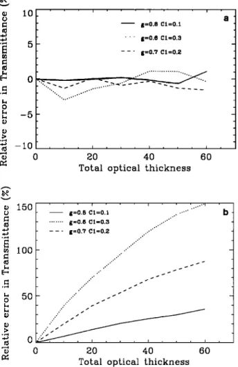
from 0 to 60. Figure 8a shows the relative difference for the

global transmittance of the inhomogeneous clouds estimated

from the equivalent optical thickness and two-stream approx-

! ' ß ' i ' ' ' !

g--O.8 C1--O.1 ... g=0.6 C1=0.3 --' g=0.7 C1=0.2

•0 40 60

Total optical thickness

i ! --1 ...- g=O.8 CI=O.I ...

g=O.8

C1=0.3

...-'"'""

Total optical thickness

Figure 8. Comparison of the relative difference of the global

transmittance of inhomogeneous clouds estimated from (25)

with those obtained under the homogeneous cloud assump-

tion. The inhomogeneous clouds are generated for total optical

thickness varying from 0 to 60 with three sets of information

codimensions and asymmetry factors: (C• = 0.1, # = 0.8),

(C1 = 0.2, # = 0.7), and (C• - 0.3, # = 0.6) (a) Relative

difference between the global transmittances estimated from

(25) and those estimated with the DART model as a function

of the total optical thickness of the clouds for the three types

of inhomogeneous clouds. (b) Relative difference between the

global transmittances of the inhomogeneous clouds estimated

under the homogeneous cloud assumption with those esti-

mated with the DART model as a function of the total optical

thickness for the same clouds as in Figure 8a.

imation. This relative difference is less than about 3%. Figure 8b shows the relative difference for the same inhomogeneous clouds but without taking account of the cloud inhomogeneity.

The bias between homogeneous and inhomogeneous transmit-

tance increases with the total optical depth and C1, and it may

attain 150% for optically thick and very inhomogeneous clouds

(Figure 8b). Thus much of the effect of heterogeneity can be

captured by the introduction of the effective optical thickness

in two-stream solutions.

7. Transmittance, Reflectance, and Absorption

in Multifractal Absorbing Clouds

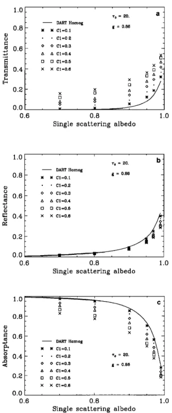
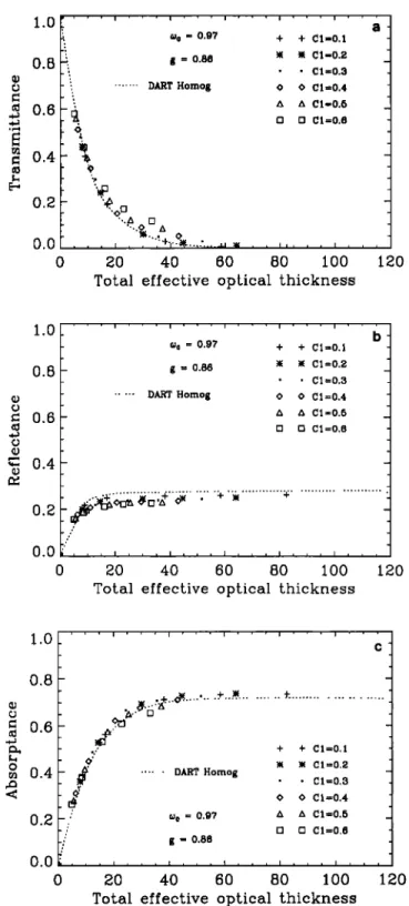
Figures 9a, 9b, and 9c present transmittance, reflectance,

29,470 BORDE AND ISAKA: RADIATIVE TRANSFER IN MULTIFRACTAL CLOUDS 1.0 0.8 0.6 0.4 0.2 0.0 0.6 DART Homog ß ß Cl=0.1 ß ß C1=0.2 O O C1=0.3 A A C1=0.4 [] o C1=0.5 x x C1=0.6 x [] 'r o = 20. g = 0.86 X O- D - 0.8 1.0

Single scattering albedo

1.0 0.8 0.6 0.0 0.6 i

ß

r o = 20.

b

ß ß CI=0.1

g = 0.86

[] o 01=0.5

Single scattering albedo

1.0 0.8 c 06 - 0.4 0.2 0.0

ß ß Cl=O.1

__

x

ß ß 01=0.2

•'o

= 20.

X

D D 01=0.5

Single scattering albedo

Figure 9. Variations of the (a) transmittance, (b) reflec-

tance, and (c) absorptance of inhomogeneous clouds as a func-

tion of the single-scattering albedo too for different values of

the information codimension C 1. The total optical thickness of

the clouds and the asymmetry factor of the scatterers are kept

constant at 20 and 0.86, respectively.

geneous clouds with ro = 20 and g = 0.86. We varied too from

0.7 to 0.99 and C1 from 0 to 0.6.

The transmittance increases and the reflectance decreases as

the cloud inhomogeneity increases from C1 = 0 to C1 = 0.6

(Figures 9a and 9b) for a fixed to o. These variations are qual-

itatively the same as those obtained for the nonabsorbing,

inhomogeneous clouds. The transmittance of an inhomoge-

neous cloud increases by an extra transmittance that depends

on C 1 and too. For a given C 1 this increase is significantly larger

for the interval 0.9 < too < 0.97 than outside it, but the mag-

nitude of this increase does not exceed 15%. The effect of

inhomogeneity on the reflectance differs significantly from the

effect on the transmittance. It lessens rapidly as too decreases

from 1 to 0.7, because the reflectance of a homogeneous cloud

itself varies very rapidly with too. The cloud inhomogeneity has

a larger effect, in both absolute and relative value, on the

transmittance than on the reflectance, but this feature may

depend on the value of g.

As for the absorptance, an inhomogeneous cloud absorbs

less energy than a homogeneous cloud with the same total

mass of the scatterers (Figure 9c). As too decreases from 0.99 to

0.80, the absorptance increases from 0.23 to 0.95 for a homo-

geneous cloud and from 0.18 to 0.78 for an inhomogeneous

cloud with a C 1 of 0.6. Hence the absorptance of highly inho-

mogeneous clouds with a moderate optical thickness is smaller

than that of the corresponding homogeneous clouds by 20 to 30%. These features are due to the fact that increasing inho-

mogeneity enlarges the area with small local optical thickness

through which light is preferentially transmitted and reduces

the area with large local optical thickness from which light is

preferentially reflected.

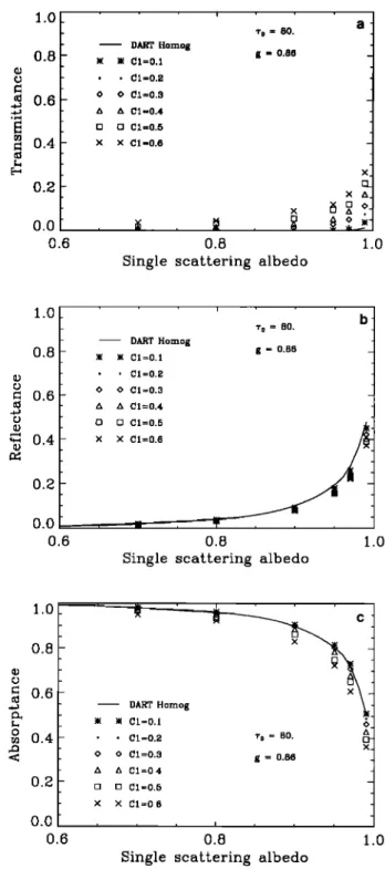
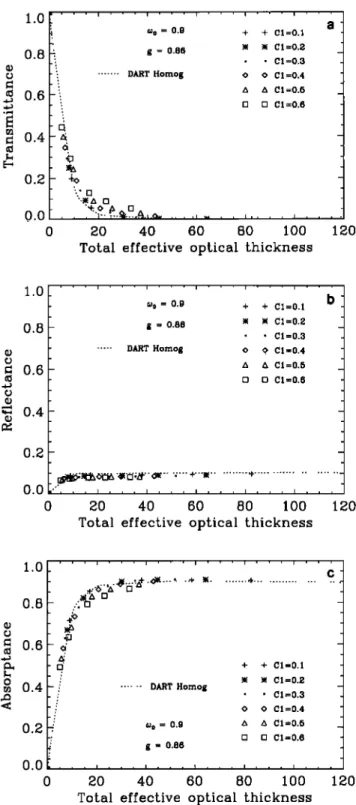
Figures 10a, 10b, and 10c present the variation of the trans-

mittance, reflectance, and absorptance as a function of the

single-scattering albedo for the inhomogeneous clouds with

the same characteristics as in Figure 1, but with a total optical

thickness of 80. The transmittance and reflectance (Figure 10a

and 10b) show variations with the cloud inhomogeneity similar

to those in Figure 9a and 9b. The transmittance still changes

significantly with the cloud inhomogeneity for a too close to 1,

while its variation with C 1 lessens rapidly in amplitude for too

less than 0.9. This feature differs from that observed above for

the clouds with a total optical thickness of 20.

The reflectance from the clouds with r o = 80 does not differ

from that obtained for the clouds with ro = 20. This suggests that the energy is reflected by the upper part of the cloud

whose optical thickness is less than 20. Therefore adding more

absorbing scatterers does not affect the amount of reflected

energy. An optically very thick cloud absorbs almost all non-

reflected energy, except in the case with too very close to 1. As

too decreases from 0.99 to 0.80, the absorptance increases from

0.48 to 0.97 for a homogeneous cloud and from 0.36 to 0.93 for

an inhomogeneous cloud with a C 1 of 0.6. Hence moderate to

high cloud inhomogeneity generally reduces the absorptance

from its homogeneous cloud value. However, the magnitude of

the effect is much smaller than the previous case (% = 20),

except for a too very close to 1. This implies that cloud inho-

mogeneity is not a pertinent physical factor for the reflectance

for a highly absorbing cloud.

A close examination of Figure 10c shows that the ab-

sorptance of an inhomogeneous cloud with a small C 1 (C 1 <

0.2) is equal to or slightly higher than the absorptance of a

homogeneous cloud with the same optical characteristics. This

feature is quite different from that obtained for the same in-

homogeneous clouds with a smaller total optical thickness of

20.

The conservation of the energy derives the expressions

BORDE AND ISAKA: RADIATIVE TRANSFER IN MULTIFRACTAL CLOUDS 29,471

Ain h -- 1 - [Tinh(co0, g, C1) q- Rinh(co0, g, C1) ]

= Ahom- [STinh(co0, #, C•) + 8Rinh(co0, #, C•)] (30b)

where Ax, Tx, and Rx are the absorptance, transmittance and

reflectance of the cloud, respectively, the index x designating

the homogeneous (hom) or inhomogeneous (inh) cloud.

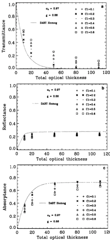
Figures 11a, lib, and 11c show the relative difference, de-

fined by (Aho m -- A inh)/Ahom, of the absorptance between

inhomogeneous and homogeneous clouds with total optical

thickness of 20, 50, and 80, respectively.

For moderate and large cloud inhomogeneity (C• > 0.2),

the relative difference generally increases as Wo approaches to

1. A highly intermittent inhomogeneous cloud (C• > 0.4)

absorbs 10-40% less energy than a homogeneous cloud for

ro = 20 and 5-30% less for ro = 80), while a slightly or

moderately inhomogeneous cloud (0.2 < C• < 0.4) absorbs

5-20% less energy for ro = 20 and 2-10% less for ro = 80). The

relative difference increases with COo because the decrease of

the absorptance is large enough to compensate the lessening

inhomogeneity effect as COo approaches 1.

For the inhomogeneous clouds with C • smaller than 0.2, the

cloud inhomogeneity tends to increase systematically the ab-

sorptance of the clouds with a total optical thickness larger

than 50 and COo larger than 0.85. However, the increase is less

than 5%, much smaller than expected. This result agrees with

that obtained by Barker [1992] for monofractal clouds with a

total optical thickness larger than 40. This increase happens

because the cloud inhomogeneity enables photons to penetrate

deeper into the clouds, but these photons cannot come out

from the clouds owing to the large optical thickness and are

finally absorbed into the clouds.

For a cloud with a small to moderate optical thickness (to <

30) the effect of inhomogeneity on the transmittance is larger

than that on the reflectance (Figures 12a and 12b), so the sum

8Tinh + 8Rinh is always positive. Consequently, the ab-

sorptance of an inhomogeneous cloud is always smaller than

that of a homogeneous cloud with the same total optical thick-

ness.

For an optically thick cloud with a total optical thickness

(to > 50), the situation becomes more complicated. The cloud

inhomogeneity always decreases the reflectance. However, the

reflectance of an optical thick cloud does not differ very much

from that of a cloud with an optically moderate thickness

because the energy is reflected mostly by the upper part of the

cloud. Nonreflected energy penetrates into the cloud, but the

transmittance rapidly approaches zero for a weakly inhomoge-

neous cloud with COo less than 0.95. Consequently, the nonre-

flected energy is trapped into the cloud and is finally absorbed

by the cloud scatterers. In this case, we have the sum •Tin h q-

•Rin h negative, which corresponds to the increased ab-

sorptance. For an inhomogeneous cloud with a large C•, the

inhomogeneity effect allows a small amount of the energy to

still be transmitted through the cloud, and this effect remains larger than the negative effect on the reflectance. Therefore the sum •rin h q- •Rin h remains positive, and the absorptance decreases because of the cloud inhomogeneity. Radiative

fluxes are computed again for the same clouds, but with larger

total optical thickness ro = 80 (Figure 1 lc). Results show that

the absorptance of an inhomogeneous cloud can be larger than

the absorptance of a homogeneous cloud with the same optical

thickness by 5%. Therefore how the cloud inhomogeneity af-

fects the radiative properties of a cloud depends not only on

1.0 0.8 o.a ,•,1 • 0.4 0.2 0.0 0.6 DART Homog C1=0.1 C1=0.2 C1=0.3 C1=0.4 C1--0.6 80. 0.86 x 0.8

Single scattering albedo

x 1.0 1.0 0.8 0.6 0.4 0.2 0.0 0.6 i

7o

= 80.

b

Single scattering albedo

1.0 0.8 c 06 _. 0.4 0.2 80. A X. 0.86 DART Homog ß ß Cl=o.1 ß ß Cl=O.a o o C1=0.3 a a C1=0.4 [] [] 01=0.5 x x C1=0.6 I 0.8

Single scattering albedo

0.0

0.6 1.0

Figure 10. The same as Figure 9, but for a total optical

thickness of 80.

the scattering properties of the scatterers and the total optical

thickness of the cloud, but also on the characteristics of the

inhomogeneity. Hence we have to be careful to generalize this

result for all types of inhomogeneous clouds because the mul-

tifractal medium has a very specific distribution of fluctuations.

8. Application of the Effective Optical Thickness

to Inhomogeneous Absorbing Clouds

For nonconservative scattering we have defined an effective