Dynamic properties of seawater surfactants

(1)

Dynamic Properties of Seawater Surfactants

by

John Thomas Mass

Submitted to the Department of Ocean Engineering in Partial Fulfillment of the Requirements for the Degree of

Masters of Science in Ocean Engineering at the

Massachusetts Institute of Technology February 1996

Signature of Author

Detartment of Ocean Engineering January 20, 1996

Certified by

Jerome Milgram Professor of Ocean Engineering Thesis Supervisor

Accepted by__

A. Douglas Carmichael Professor of Ocean Engineering Chairman, Department of Ocean Engineering Graduate Committee

r~C~r r--I-ml

'V K'::

FEB 2 0

1997

-IF ILa

(2)

Dynamic Properties of Seawater Surfactants

by

John Thomas Mass

Submitted to the Massachusetts Institute of Technology on January 30, 1995 in partial fulfillment of the requirements for the degree of

Master of Science in Ocean Engineering

Abstract

The relative calm in ship wakes and its persistence for long periods raises questions regarding energy dissipation mechanisms by which surface elevation waves are damped. Wave field disturbances caused by propeller and boundary layer turbulence can readily explain the absence of waves immediately astern but fail to explain their absence many shiplengths astern. A possible mechanism to explain the lack of high frequency surface elevation waves is the presence of surface active agents, surfactants. Surfactant collection into continuous sheets or disturbing previously formed sheets can readily change the decay rates of surface elevation waves through changes in surface tension, elasticity and possibly surface viscosity. In addition to shipwakes, the rheological behavior of a surface film can influence wave growth due to wind.

Elastic properties are typically determined experimentally through quasi-static measurement of the film's pressure-area isotherm but recent discussions have raised the question of whether the quasi-static properties explain the dynamic behavior of naturally occurring ocean surfactants. The objective of this research is to determine if the quasi-static elastic properties (Gibbs' elasticity) of seawater films adequately predict the dynamic behavior of natural sea surface films. Specifically, the dynamics of the films when they undergo distortions from both transverse and longitudinal waves.

The quasi-static elastic properties were found to change with repeated compression resulting in a " work hardening" of the film. However, once determined the quasi-static elasticity predicts the dynamic behavior of natural surface films.

Thesis supervisor: Dr. Jerome Milgram Title: Professor of Ocean Engineering

(3)

ACKNOWLEDGMENTS

Professionally, I would like to thank Professor Jerome Milgram for supervising the work that lead to this thesis. He is everything a MIT professor should be, intelligent and hard working. I would like to thank the Office of Naval Research for providing funds for this project.

During the course of this work I have had the opportunity to work with several people in the MIT community. Dr. Hasan Olmez proved to be a great intellectual big brother when I needed help with computational problems and finding my way around MIT. Noah Eckhouse taught me about high frequency electronic noise at MIT and helped me adjust to the Boston area. Soren Jensen enhanced my knowledge of Denmark and showed me a few tricks on the lathe. When the aforementioned left the LAB to pursue other interests Greg Thomas, Nicole Suoja and Jess Riggle moved in with refreshing zeal and continued to make the place a pleasant working environment. Cindy Dernay deserves credit as a person who can get things done and get almost anything delivered by the next day. Craig Schull spent the summer earning my respect. He is, without a doubt, the best UROP I have ever worked with at MIT.

Personally, I would like to thank my parents and numerous brothers and sisters for somehow helping to make me what I am.. During my stay at MIT I joined another family; James and Diana Brown thank you for your daughter and support in our endeavors.

Finally, I would like to thank my wife Michele, whose love, support and counsel means the world to me.

(4)

LIST OF FIGURES

FIGURE 2.1 RELATIONSHIP BETWEEN LONGITUDINAL WAVE NUMBER, FREQUENCY AND

ELASTICITY FOR: y = 68.0 mN / m, e' = 0 mN / m / sec. ... 14

FIGURE 2.2 RELATIONSHIP BETWEEN CHANGES IN SURFACE TENSION, ELASTICITY AND FREQUENCY FOR d = 40 cm, x = 7 cm, y = 68.0 mN / m, e' = 0 mN / m / sec. ... 17

FIGURE 2.3 RELATIONSHIP BETWEEN PHASE, ELASTICITY AND FREQUENCY FOR d = 40 cm, x = 7 cm, y = 68.0 mN / m, E' = OmN / m / sec. ... 18

FIGURE 2.4 RELATIONSHIP BETWEEN DECAY RATE, ELASTICITY AND FREQUENCY FOR y = 68.0 mN / m, e " = OmN / m / sec ... 19

FIGURE 2.5 RELATIONSHIP BETWEEN NORMALIZED DECAY RATE, ELASTICITY AND FREQUENCY FOR: y = 68.0 mN / m, e'= OmN / m/ sec. ... 20

FIGURE 2.6 COMPRESSION MODEL OF SURFACE FILM ... 21

FIGURE 2.7 QUASI-STATIC PRESSURE-AREA ISOTHERM... ...22

FIGURE 2.8 ELASTIC PROPERTIES FROM QUASI-STATIC PRESSURE-AREA ISOTHERM...23

FIGURE 3.1 LONGITUDINAL WAVE TROUGH ... ... 24

FIGURE 3.2 W AVE DECAY TANK...25

VARIATION IN SURFACE TENSION: VARIATION IN SURFACE TENSION: VARIATION IN SURFACE TENSION: VARIATION IN SURFACE TENSION: VARIATION IN SURFACE TENSION: VARIATION IN SURFACE TENSION: VARIATION IN SURFACE TENSION: VARIATION IN SURFACE TENSION: VARIATION IN SURFACE TENSION: OLEYL ALCOHOL y = 68.0 mN / OLEYL ALCOHOL y = 67.0 mN / OLEYL ALCOHOL y = 70.0 mN / m OLEYL ALCOHOL y = 70.0 mN / m OLEYL ALCOHOL y = 69.0 mN / m OLEYL ALCOHOL y = 70.0 mN / m COHASSET SEAWATER y = 69.0 mi COHASSET SEAWATER y = 68.0 mi COHASSET SEAWATER y = 69.0 mi m ...29 m ...29 ... 30 ... 30 ...3 1 ...3 1 N / m ... 32 N / m ... 33 N /m ... 33

FIGURE 5.10 VARIATION IN SURFACE TENSION: WOODS HOLE SEAWATER y = 70.0 mN / m 34 FIGURE 5.11 VARIATION IN SURFACE TENSION: WOODS HOLE CONCENTRATE y = 70.0 mN / m ... 35

FIGURE 5.12 VARIATION IN SURFACE TENSION: WOODS HOLE CONCENTRATE y = 70.0 mN / m ... ... 36

FIGURE 5.13 VARIATION IN SURFACE TENSION: WOODS HOLE CONCENTRATE y = 69.0 mN / m ... ₃₆

FIGURE 5.14 VARIATION IN SURFACE TENSION MAGNITUDE DUE TO SURFACE VISCOSITY 37 FIGURE 5.15 VARIATION IN SURFACE TENSION PHASE DUE TO SURFACE VISCOSITY ... 38

FIGURE 6.1 TRANSVERSE WAVE DECAY RATES: CLEAN WATER y = 72.0 mN / m ... 40

FIGURE 6.2 TRANSVERSE WAVE DECAY RATES: CLEAN WATER y = 72.0 mN / m ... 41

FIGURE 6.3 TRANSVERSE WAVE DECAY RATES: CLEAN WATER y = 72.0 mN / m ... 41

FIGURE 6.4 TRANSVERSE WAVE DECAY RATES: OLEYL ALCOHOL y = 67.0 mN / m ... 42

FIGURE 6.5 TRANSVERSE WAVE DECAY RATES: COHASSET SEAWATER y = 69.0 mN / m ....43

FIGURE 5.1 FIGURE 5.2 FIGURE 5.3 FIGURE 5.4 FIGURE 5.5 FIGURE 5.6 FIGURE 5.7 FIGURE 5.8 FIGURE 5.9

(8)

FIGURE 6.6 TRANSVERSE WAVE DECAY RATES: COHASSET SEAWATER y = 72.0 mN / m ....43

FIGURE 6.7 TRANSVERSE WAVE DECAY RATES: COHASSET SEAWATER y = 71.0 mN / m ....44

FIGURE 6.8 TRANSVERSE WAVE DECAY RATES: COHASSET SEAWATER y = 69.0 mN / m ....44

FIGURE 6.9 TRANSVERSE WAVE DECAY RATES: WOODS HOLE SEAWATER y = 70.0 mN / m 4 5 FIGURE 6.10 TRANSVERSE WAVE DECAY RATES: WOODS HOLE CONCENTRATE y = 70.0 mN / m ... 46

FIGURE 6.11 TRANSVERSE WAVE DECAY RATES: WOODS HOLE CONCENTRATE y = 69.0 mN / m ... 46

FIGURE 6.12 VARIATION IN DECAY RATE DUE TO SURFACE VISCOSITY ... 47

FIGURE 7.1 ELASTIC PROPERTIES OF OLEYL ALCOHOL: I ... 49

FIGURE 7.2 ELASTIC PROPERTIES OF OLEYL ALCOHOL: II ... 49

FIGURE 7.3 ELASTIC PROPERTIES OF COHASSET SEAWATER: I ... 50

FIGURE 7.4 ELASTIC PROPERTIES OF COHASSET SEAWATER: II ... 50

FIGURE 7.5 ELASTIC PROPERTIES OF WOODS HOLE SEAWATER ... 51

FIGURE 7.6 ELASTIC PROPERTIES OF WOODS HOLE CONCENTRATE ... ...51

FIGURE A. 1 SKETCH OF LONGITUDINAL WAVE TROUGH ... 54

FIGURE A.2 PROGRAMS AND DATA FILES ... 63

FIGURE A.3 MEASURED PHASE ANGLE BETWEEN TRANSVERSE WAVEMAKER AND LASER SLOPE G AUGE ... ...65

FIGURE A.4 COMPARISION OF SURFACE TENSION MEASUREMENTS ... ... 65

FIGURE A.5 CHANGE IN SURFACE TENSION PHASE ERROR ... 66

FIGURE A.6 TIME DELAY SUBTRACTED FROM MEASURED PHASE ... 69

FIGURE B. 1 SKETCH OF WAVE DECAY MEASUREMENT APPARATUS...70

FIGURE B.2 SKETCH OF TRANSVERSE WAVEMAKER ... ... ... .. 72

FIGURE B.3 SCHEMATIC OF THE SINGLE-ENDED INPUT DIFFERENTIAL AMPLIFIER ... 72

FIGURE B.4 BEACH DESIGN ... 73

FIGURE B.5 ELECTRONIC BALANCE AND HEIGHT ADJUSTMENT ... 75

FIGURE B.6 LASER CARRIAGE POSITION CALIBRATION...76

FIGURE B.7 LASER SLOPE GAUGE DESIGN...77

FIGURE B.8 SAMPLE OF RAW WAVE DECAY DATA FILE ... 79

FIGURE B.9 SAMPLE PEAK-TO-PEAK SLOPE AMPLITUDE DECAY ... 80

FIGURE B. 10 FIT OF NORMALIZED LASER SLOPE DATA... 81

FIGURE C. 1 RELATIONSHIP BETWEEN PHASE AND kl . ... ... 83

FIGURE C.2 CLEAN WATER PHASE VELOCITY ... 86

FIGURE C.3 SURFACTANT WATER PHASE VELOCITY... 86

FIGURE C.4 SURFACTANT WATER PRESSURE-AREA ISOTHERM ...87

(9)

LIST OF SYMBOLS

SYMBOL

k

k a p g 0) k T E E' kL y' Yo phase(y') x d a ( 1-I F Lp, V, V,_p) DISCRIPTION Vertical Displacement Horizontal Displacement Complex Wavenumber Real Wavenumber

Imaginary Wavenumber (Decay Rate) Wavelength Pi - 3.14159265 Density Gravity Circular Frequency m2 ₌_k2 _{- iwpl/yU}

Dynamic or Absolute Viscosity Kinematic Viscosity

Surface Tension Complex Elasticity Gibbs' Elasticity Surface Viscosity

Initial Transverse Wavenumber Initial Longitudinal Wavenumber Refined Transverse Wavenumber Refined Longitudinal Wavenumber Change in Surface Tension

Initial Surface Tension

Phase Relationship between Longitudinal Wavemaker and Fluid Distance from longitudinal wavemaker to a Point on the Fluid Distance from Longitudinal Wavemaker to Opposite wall Transverse Wave Decay for Clean Water

Film Pressure

Force acting on Wilhelmy Plate Length of Wilhelmy Plate Group Velocity

(10)

1. Introduction

The presence of certain compounds on the sea surface alters propagation characteristics of short surface waves. The compounds, generated from phytoplankton by-products and land run-off, can form a monomolecular sheet with elastic properties. The elastic sheet supports the propagation of transverse (gravity-capillary) and longitudinal surface waves. When a transverse wave exists on a film-covered region, the combination of longitudinal and transverse waves that must exist to satisfy the boundary conditions can increase the transverse wave dissipation. This happens because of phase differences in the longitudinal and transverse wave motions which can enhance viscous dissipation in the boundary layer just beneath the surface film. The surface, if wind driven and rough, becomes smoother when a surface film is present.

1.1. Background

Recorded observations of the above phenomenon were noted in ancient Greece and Rome by philosopher-scientists. However, scientific understanding did not begin until late in the

19th century when Italian physicist C. Marangoni documented fluid -fluid interactions at the

air-liquid interface. A qualitative understanding was offered by Aitken 1883 and summarized by Adam 1941. Quantitative analysis by Dorrestein 1951 and extensive experimental data on 'oils' followed with work by Mann and Hansen 1963, Lucassen and

Hansen 1966, and Hansen and Ahmed 1971.

In 1978 additional interest was focused on the field due to developments in synthetic aperture radar and the use of radar backscatter to measure spectral properties of large areas of the ocean. Shipwakes and oil slicks could now be tracked remotely from air and space. Observed phenomena became measured phenomena. However, understanding the data required evaluation of surface properties. An effort was made to catalogue the elastic properties of a wide variety of surface films taken from the sea to the laboratory [Barger,

1984 and Bock and Frew, 1993]. Natural Films were shown to have varying composition and quasi-static elastic properties. The films showed an increase in elasticity or " hardening" with repeated compression. Some in-situ experiments were carried out on man made slicks composed of a compound with known elastic properties [Alpers and

Huhnerfuss 1989].

An open question was whether the quasi-static film properties properly describe the film dynamic behavior which influenced seawaves. The result of Hunerfuss, Lange and Walters [1985] suggested that dynamic elasticity and surface viscosity at seawave frequencies may not have quasi-static values, even for pure substance films. This information contributed to stimulating the present study reported here.

1.2. Objective

The objective of this research is to determine if the quasi-static elastic properties (Gibbs' elasticity) of seawater films adequately predict the dynamic behavior of natural sea surface

(11)

films. Specifically, the dynamics of the films when they undergo distortions from both transverse and longitudinal waves.

1.3. Approach

We intended to accomplish our objective by:

A. Generating a baseline using a known compound (Oleyl Alcohol) whose quasi-static properties adequately predict its dynamic properties

B. Collecting samples of film covered seawater, transporting it to our laboratory, and spreading the film on wave apparatus in a natural state.

C. Measuring the quasi-static elastic properties of the surface film

D. Measuring dynamic properties of the film for a range of frequencies from 0.4 to 20 Hz

Initial samples were collected from the Little Harbor inlet near Cohasset, Ma (north shore Cape Cod) on the incoming tide. In an effort to prevent the films from changing due to biological growth/decay samples were collected transported and tested within 24 hours. In addition, comparisons were made between samples poisoned with sodium azide and samples not poisoned. The film properties were the same, whether poisoned or not, for films tested within 24 hours.

Near the completion of testing Nelson Frew and Robert Nelson of Woods Hole Oceanographic Institute provided surface film concentrate from a salt pond near Falmouth Ma. (a.k.a. Woods Hole Concentrate). Water samples were collected from the salt pond and concentrated in a centrifuge. The concentrate, eluted with methanol [Frew and Nelson, 1992], was spread on tap water and evaluated for quasi-static and dynamic properties. In an effort to establish a baseline for the concentrate evaluations film covered water samples were collected from the salt pond and evaluated in the same manner as the Cohasset samples.

2. Theory

2.1. Dynamic Properties of Transverse and Longitudinal Waves

Two types of surface waves can be supported at the air-water interface. The first, transverse waves, are the general water waves most people are familiar with; the air-water interface oscillates vertically and the vertical motion propagates in the plane of the air-liquid interface. To the observer in the global reference frame, as the wave passes particles trace out a circular pattern in deep water and an elliptical pattern in shallow water.

The second type, longitudinal waves , exist when oscillatory motion is almost completely parallel to the air-water interfacial plane. In this case the horizontal motion is an order of

(12)

magnitude greater than the vertical motion of the fluid. To the stationary observer a particle floating on the surface simply moves back and forth as the wave travels parallel to the air-liquid interface. These waves require an elastic surface.

In the case of a film covered surface, the fluid can support both types of waves simultaneously.

For both transverse and longitudinal cases two dimensional wave theory gives us a displacement relationship of the form:

e=

oei(kx-o) (2.1a)

in the z direction and

= 4ei(kx-a)

(2.1b)

in the x direction with transverse waves having / 0(1) and longitudinal waves having a much smaller ratio of / I. The equations relate wavenumber, distance, circular frequency and time to free surface displacement. The complex wavenumber, k, is equal to k + ia. The real portion represents the spatial wavenumber, k, and is related to the wavelength by

2 = 27r/ k. The imaginary portion, a, represents the spatial decay rate.

The dispersion relationship between k and measurable fluid properties is given by:

(pwo2

_ 3 _ pgk)(po 2 mk2_E)

_ k3(3 + pgk) + 4ip1(gw 3_k2 ₊₄₂₀₂ 3_(m- _{k)= 0} (2.2)

[Hansen and Ahmed, 1971] where: m2 _=k2_{- ip} _/

(2.3) Using gravity, g, and measuring the density, p, and viscosity, / , of the underlying fluid and surface tension, y, and elasticity, E, for the film covering the air-water interface one can determine the corresponding wavenumber for any desired frequency by finding the roots of Equation 2.2 which is sixth order in k . A typical numerical method is to estimate the locations of valid roots then use Newton's Method, or the leading term in an expansion, to refine the root locations. Since the roots must satisfy the boundary conditions of zero displacement at infinite depth several roots can be discarded as improper solutions.

In the case where the elasticity, E, is equal to zero, equation 2.2 simplifies to:

(pow2 _- 3 _{_ pgk)(po}2) _{+ 4ip12o}3_k2 ₊₄

1 22 2 k3(m- k) = 0 (2.4)

and the roots are located very close to the roots of first term which has the familiar form: 12

(13)

(pw

2

_-

₃

_{-pgkf) = 0}

When an elastic film is present the elasticity, E, will not be equal to zero. Furthermore the elasticity may have a real and imaginary part forming the complex term:

E= E+ ie'ao (2.6)

where the real part of the elasticity, e, represents pure elastic or quasi-static behavior, while the imaginary part ,E', is the film surface viscosity.

Hansen and Ahmed [Waves at Interfaces, 1971] show that the solution for transverse and longitudinal wavenumbers are approximated by:

(2.7)

and

respectively. Then the roots are refined to:

(2.8)

, Ek 2 ( 3 + pgk) -4ipoam3 _k (3* 2 + pg)(pw2 -42 2k 2 (m- k) . - mk 2 - _k=_k" , k (k' + pgk) -4ip.uo 3_{k -41/.}2 _k2_{(m- k)1} 2mkt(pw2 3 _{- pgk)} k=oL (2.9) (2.10)

In both cases the real portion of k gives information regarding the wavelength, A. = 27r/ k,

while the imaginary portion provides information about the decay rate, a. Figure 2.1 shows the dependence of longitudinal wavenumbers, kL, on frequency and elasticity.

The first order correction to wavenumber in equation 2.10 is small and there relationship between k and i; as the elasticity, e, decreases the wavenumber, resulting in shorter wavelengths. When the water is clean, e =0, the wavelength is zero.

is an inverse

k, increases,

longitudinal

In the case of transverse waves, the estimated location of the roots in equation 2.7 has only a real component which is independent of elasticity. The corrected wavenumber, k ,

calculated in equation 2.9 has a relatively small dependence on E such that the real portion of the root can be estimated by I((o,g,y,p,-)= I((o,g,y,p). The change in elastic

(2.5)

(14)

properties will result in dramatic changes in longitudinal wavelength while leaving the transverse wavelength largely unaffected. The imaginary parts of the transverse and longitudinal wavenumbers provide information regarding the decay rates of the respective waves, both have a strong correlation with elasticity. The dependence of longitudinal waves on elasticity is discussed below and transverse waves in section 2.2.

Relationship between Longitudinal Wavenumber, Frequency and Elasticity

. 6 E 1 E C~ e 0 1 2 3 Frequency [Hz]

Figure 2.1 Relationship between Longitudinal Wave Number, Frequency and Elasticity for:

y = 68.0 mN / m, E' = 0 mN / m/ sec.

2.1.1. Longitudinal Wave Decay and Variations in Surface Tension

In the open ocean a film covered surface with elastic properties will have longitudinal waves generated from transverse waves distorting the equilibrium surface film. One method of studying longitudinal waves is to de-couple them from transverse waves through the use of a longitudinal wavemaker and wave tank or trough. The following discussion is for a film covered surface in a wave tank equipped with a longitudinal wavemaker.

When a continuous monomolecular sheet or monolayer film exists, longitudinal waves can be generated without causing significant vertical particle motion by displacing surfactant molecules that form the monolayer film in the plane of the air-water interface. The waves are generated by horizontal displacement of the surfactant molecules with a film barrier. The barrier is placed on top the longitudinal wave tank piercing the monolayer with minimum penetration of the underlying fluid. Oscillating the film barrier horizontally

(15)

displaces the surface molecules. Motion of the bar causes displacement of particles on the air-water interface making up the surface film. A longitudinal wave is generated.

From classical wave theory, the displacement of a surface particle must satisfy equation 2.1. using the longitudinal wavenumber, kL, derived in equation 2.10. Furthermore, the particles on the surface near the wavemaker must have a displacement nearly equal to the

wavemakers. If the displacement of the film barrier (wavemaker) is of the form:

4 = Ae i(7l/ 2 - ox) (2.11)

The displacement of the film particles near the wavemaker will have to satisfy the same expression. Due to the finite length of the trough, reflection can occur off the wall opposite the oscillating film barrier. Particles near the wall will have the same displacement as the wall, zero. If the solution is to account for one reflection off the wall it will be of the form:

= Bei(k x-_al) _{+ Cei(}c- lx-a₎ _(2.12)

The first term on the right represents a wave traveling in the +x direction (right) and the second term represents a wave traveling in the -x direction (left). From the first boundary condition, equation 2.11, film displacement must equal film barrier displacement near the film barrier, one gets the equality:

4x=0 = _Aei(-r/2-) _{= Bei(i}_- ₊_Cei'(-) _(2.13)

or

B + C = Aei(-; /2) _(2.14)

The second boundary condition dictates that the fluid displacement at the wall must zero. If

d is the distance between the wavemaker and far wall and the distance is much larger than

the wavemaker amplitude, A, the boundary condition at d is:

4x=d = Bei(kLd-) + Cei(-kLd-a) =

0

(2.15)

or

Bei(kLd) + Cei(- kLd) =

0 (2.16)

which gives two equations with two unknowns. Rearranging equation 2.14:

C = Ae i(-r/2) - B (2.17)

(16)

B = Ae i/2 e-Ld _(2.18)

eikLd - e ikLd

Substituting the coefficient B back into equation 2.17 and simplifying yields:

C= Aei • e id (2.19)

ikLd -ikd

With the coefficients calculated one can state the specific solution for surface particle displacement at any point on the air-water interface.

-ikLd ikLd

=

Ae i/12

e

- ed i(kLx-()

+

Ae

irl2

e

i(-kx-) (2.20)

eikLd - eiLd ei _ e(i.Ld-d

or simplified;

[

e-ikLd eik

L_d

SAei(/2--ikd eikLx

+

e-ikx

(2.21)

As the longitudinal wave travels in x, the particle motion causes the interface film to distort (stretch and compress). The elastic properties of the film dictate the local changes in surface film pressure and surface tension from the static equilibrium as the film is stretched and compressed to a larger and smaller area. The variation in surface tension, y', is the elasticity multiplied by the horizontal strain for simple elastic behavior:

di e-ikLd e ik

Ld

y'

=

ikd L

eikLX

i ikLd e -ikLx

(2.22)

dx eik d -ik d ikLd -ikd

The fact that elasticity, E, and wavenumber, k can be complex, dictates y' can have real and imaginary parts or a magnitude and phase. The magnitude of y'is the amplitude of variations in surface tension and the phase represents the phase shift of variations in surface tension at a distance x from the film barrier with respect to strain. Equation 2.22 shows sinusoidal oscillation of the longitudinal wavemaker generates sinusoidal variations in dilation and surface tension. The variation in surface tension is affected by the longitudinal wave and elastic properties of the film. The varying surface tension corresponds to:

Y= Y0 + y'Icos[phase(y')- at] (2.23)

Several methods exist to measure variations in surface tension. One method measures the changes in surface tension with minimum interference of the film present at the air-water

(17)

interface [Sohl, Miyano and Ketterson, 1978]. Details of the device we developed are given in section 3 and appendix A.

The relationship between the magnitude of surface tension variation, elasticity and frequency at one position in the trough is shown in figure 2.2. The change in surface tension is normalized with respect to the amplitude of the oscillating film barrier (longitudinal wavemaker). This allows one to discern small changes in surface tension at the higher frequencies.

Relationship between Changes in Surface Tension, Elasticity and Frequency

1 2 3 4 5

Longitudinal Wavemaker Frequency [Hz]

Figure 2.2 Relationship between Changes in Surface Tension, Elasticity and Frequency for

d = 40 cm, x = 7 cm, y = 68.0 mN / m, E'= 0 mN / / sec.

Figure 2.3 shows the variations in phase dependence on elasticity and frequency at the same position as figure 2.2. The phase difference of the change in surface tension with respect to

the oscillating film barrier is also sensitive to changes in elasticity.

After measuring the parameters which describe the fluid and surfactant, one can calculate theoretical values for the longitudinal wavelength, the displacement of particles on the film between the air-water interface and local variations in surface tension. The combination of the three allows one to compare theoretical dynamic behavior of a film with measured behavior.

Unfortunately, generating longitudinal waves at frequencies above 4 Hz without generating transverse waves is difficult. Transverse waves form from meniscus forming on the film

= 40 mN/m

= 30 mN/m

= 20 mN/m

(18)

barrier and the bar's penetration into the underlying fluid. Analyzing dynamic behavior for higher frequencies requires another approach.

Relationship between y' Phase, Elasticity and Frequency

1 2 3 4 5

Longitudinal Wavemaker Frequency [Hz]

Figure 2.3 Relationship between Phase, Elasticity and Frequency for

d = 40 cm, x = 7 cm, y = 68.0 mN / m, e' = OmN / mi /sec.

2.1.2. Transverse Wave Decay

In the laboratory, transverse waves can be generated with frequencies ranging from -4 Hz up to several hundred Hz with relative ease. Throughout this range the wave characteristics depend on surface tension and elasticity making transverse waves an ideal means to study surface film properties. As stated earlier, the real portion of the roots in the transverse dispersion relation (equation 2.9) are relatively insensitive to changes in elasticity. However, recalling equation 2.1 and 2.2

•= oei(ex-v)

= e i(iok x-_o)

(2.1) (2.2) the imaginary portion of the wavenumber, k, is the real spatial decay rate. Equation 2.7 gives us an approximation or starting value of k that can be corrected using equation 2.9.

= IV mI/m : = 20 mN/m = 30 mN/m = 40 mN/m II - · -d 4• •TI

(19)

However, in the case of waves with frequencies in the range 4 - 15 Hz the gravitational effects must be included when determining the approximate location of the roots.

(p

2

_-

3

_{- pgk) =}

_O

_(2.5)

Rather than finding the roots of for the corresponding value of resolve the first order estimate complex wavenumber provides the real decay rate, a. Figure elasticity.

equation 2.5, given a specific wavelength, A, one can solve frequency, co, and use the combination in equation 2.9 to of the complex wavenumber, k. The real portion of the information about the wavelength and imaginary portion is 2.4 shows the dependence of decay rate on frequency and

Relationship between Decay Rate, Elasticity and Frequency

Y Q o o a ~ % _ucl E a a 0 10 20 Frequency [Hz]

Figure 2.4 Relationship between Decay rate, Elasticity and Frequency for

y = 68.0 mN / m, e'= OmN / m / sec.

Of immediate interest are the crossovers that take place between 4 - 8 Hz. Below the crossover point; low elasticities have lower decay rates but above the crossover point; low elasticities have higher decay rates. At first glance the high decay rates for films with low elasticities seem counter intuitive, but the decay is related to the phase between the film motion and the underlying fluid motion. The actual dissipation occurs in the upper water boundary layer. The relative phases are frequency dependent resulting in the crossovers.

(20)

A great deal of literature regarding wave decay is presented in non-dimensional form; where the decay rate, a, is normalized by the clean water decay rate, a_o. Hansen and Ahmed [1971] give clean water spatial decay for transverse waves as:

2kwuo

ao₀ -pg _{+ 3} (2.24)

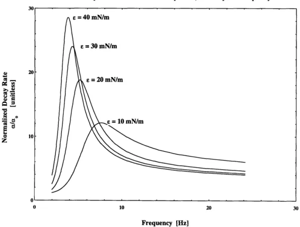
The benefits of normalizing the decay rates become apparent when reviewing data in the crossover region, 4 -8 Hz. Here the clean water decay is very small while the film covered surface continues to have a significant damping effect. Figure 2.5 illustrates the relationship between normalized decay rates, elasticity and frequency.

Relationship between Normalized Decay Rates, Elasticity and Frequency

U' ,

N o z

10 20

Frequency [Hz]

Figure 2.5 Relationship between Normalized Decay Rate, Elasticity and Frequency for:

y = 68.0 mN / m, e' = OmN / m/ sec.

Regardless of the method of viewing; gravity-capillary wave decay rates have a strong dependence upon elasticity and frequency making them suitable for evaluating film properties.

2.2. Quasi-Static Elastic Properties

Quasi-static elastic properties of surface films are determined experimentally through measurement of the pressure-area isotherms. The film pressure is the variation in surface

20

Ill · · · ·

II

V

(21)

-tension the film evokes when it forms into a continuos sheet or monolayer. In the case of elastic films, the films are usually made up of molecules with hydrophilic heads and hydrophobic tails forming into sheets one molecule thick. Present in such low concentrations the molecules are spaced widely apart and have no interaction. The surface tension is the same as the air-water interface. Sliding a film barrier compresses the molecules into a smaller surface area increases their concentration and interaction. Eventually the concentration increases to a critical level, the formation of a continuos monomolecular sheet. Any addition compression results in a drop in surface tension due to film pressure. The surface tension drops as film pressure increases. If compression continues, the resistance of the molecules to being packed closer together increases in a nonlinear relationship with increasing film pressure.

Macroscopically one can conceptualize the monolayer as a rubber sheet. Compressing it requires a sustained force, and its elastic properties result in local disturbances in pressure being transmitted trough the sheet.

Force S-'·- Wilhelmy Plate / /- Surfactant Moecule Compression Force Force Film Barrier

Figure 2.6 Compression Model of Surface Film

2.2.1. Experimental Determination of Surface Film Elastic Properties

Determining the elastic properties of a film requires accurate measurement of the film pressure. Surface film pressure, FI, is related to surface tension, y , by:

(22)

where, y,, is the clean water surface tension measured before the film forms into a continuous monomolecular sheet or monolayer film and y represents the surface tension after compression begins.

Several methods have been developed to measure surface tension. One method uses a platinum coated slide known as a Wilhelmy Plate. The plate is lowered into contact with the air-liquid boundary and the force exerted by the fluid meniscus on the plate is measured. The surface tension, y, is related to the downward force, F, exerted by the fluid on the plate by equation 3.2; where L, is the length of the plate.

F = 2L,p (2.26)

Data points are collected by adjusting the film area, lowering the plate into the water and pulling it out till the meniscus is at a near breaking point, then measuring the force with a force balance. The force and film area are converted and recorded as film pressure and surface area for each data point. Data points are collected over a range of areas where the film pressures vary from 0 mN/m, surfactant molecules sparsely located, to a point where the monolayer film is near buckling. The film area is controlled by slowly moving a barrier and waiting for the film to stabilize. A conceptual visualization is offered in Figure 2.6 and a typical pressure-area isotherm for oleyl alcohol is shown in Figure 2.7.

Pressure -Area Isotherm

Oleyl Alcohol Compression #1: 13 Sept. 1995

6.2 6.4 6.6 6.8 7.0

Log(Area [cm2

])

(23)

Once the pressure-area isotherm is collected the Gibbs' elasticity, e, of a film is determined from the definition:

dH

d[ln(area)] (2.27)

A typical approach used to calculate quasi-static elasticity is to fit the pressure-area isotherm with a mathematical function then differentiate the function. Figure 2.7 shows a 5th

order polynomial fit for the measurement of an oleyl alcohol film. Figure 2.8 shows the elasticity found by differentiating the polynomial fit.

Elasticity vs. Film Pressure Oleyl Alcohol Compression #1: 13 Sept. 1995

0 5 10 15 20

Film Pressure, H [mN/m]

(24)

3. Apparatus

Two devices were built to measure the dynamic properties of elastic films. The Longitudinal Wave Trough, figure 3.1, was built to analyze dynamic properties from longitudinal waves with frequencies up to 4.5 Hz. An 80 cm long aluminum trough held water samples. When an elastic film is present as a monomolecular sheet, oscillating the film barrier horizontally generates longitudinal waves at the surface-air interface that propagate along the trough. The longitudinal waves create local variations in surface tension. The variations in surface tension are measured by monitoring changes in wavelength of high frequency capillary waves. A transverse wavemaker generates capillary waves at 200 Hz propagating across the tank and normal to the longitudinal waves. A laser slope gauge is used to determine the time varying wavelengths of the 200 Hz transverse waves. The dispersion relationship for capillary waves, equation 2.7, is used to relate changes in wavelength to changes in surface tension.

A full explanation of the design, construction and operation of the device is given in Appendix A.

i/

/I

Film Barrier Motion Table

K

\jy

I~j

LIr

Figure 3.1 Longitudinal Wave Trough

I _;ZI

r`

(25)

The Wave Decay Tank, figure 3.2, was built to measure the dynamic properties of elastic films at frequencies between 4 and 25 Hz. A paddle type wavemaker generated 2D transverse waves. Four laser slope gauges mounted on a sliding carriage measured the amplitude decay of the transverse waves. Software calculated and averaged the four decay rates which were compared to theoretical decay rates; the imaginary portion of the transverse wavenumber, equation 2.10.

The tank was 2.4 m in length, 0.42 m in width and filled to a depth of 0.1 m. An acoustic speaker driving a wavemaker generated transverse waves. A beach minimized reflection of the transverse waves once they had passed through the data window. The electronic balance and Wilhelmy Plate were used to measure pressure-area isotherms in the calculation of the film quasi-static elasticity, and monitor the film pressure during wave decay experiments.

A full explanation of the design, construction and operation of the device Appendix B.

Sliding Carriage

is given in

Posititm Entxler

Figure 3.2 Wave Decay Tank

Both devices were equipped with components enabling the measurement of pressure-area isotherms and calculation of quasi-static elasticity.

(26)

4. Experiments and Results

Prior to testing natural films several "confidence" tests were performed on films with known characteristics. The dynamic properties of oleyl alcohol were measured in both devices and the dynamic properties of clean water, transverse wave decay rates, were measured in the Wave Decay Tank. The tests provided a baseline to ensure the devices were working properly.

4.1. Sample Collection

Seawater samples were collected from two shore based locations with free flowing connection to the ocean. Little Harbor near Cohasset, Ma. is a 100 acre pond with an inlet cross section area of approximately 150 square meters. The inlet faces the Atlantic Ocean on the north side of Cape Cod. Seawater was collected from the coastal road bridge on the incoming tide when water was near the high tide mark. The bridge forms the narrowest constriction of the inlet creating a large eddy during flood tide. The eddy naturally concentrates surface films. The samples gathered during flood tide were representative of coastal ocean surfactant. The second location was a 5 acre salt pond located near Falmouth Ma. The pond is free flooding through a narrow viaduct connecting it to Vineyard Sound. The inlet has a cross section area of approximately 3 square meters. Collection of water at the inlet during ebb tide provided surfactant of different origin than the Cohasset samples. The seawater samples were collected by immersing containers into film covered seawater. The containers were positioned with their openings piercing the surface creating a waterfall into the container. This process captured surface material. Water samples were transported to the laboratory and tested within 24 hours.

4.2. Testing Sequence

Once seawater samples were collected and transported to the laboratory experiments were conducted in the following manner

1. Fill Wave Decay Tank and Adjust Film Concentration by letting a film adsorb to the surface and compressing it with a film barrier.

a. Measure Quasi-Static Elasticity (minimum of 3 times) b. Measure Dynamic behavior for frequencies of 4.0 -25 Hz c. Measure Quasi-Static Elasticity (minimum of 2 times) 2. Wave Decay Tank and Adjust Film Concentration by compression

with a barrier.

a. Measure Quasi-Static Elasticity (minimum of 3 times) b. Measure Dynamic behavior for variations up to 4.0 Hz c. Measure Quasi-Static Elasticity (minimum of 2 times)

The characteristics of the quasi-static elasticity varied with repeated compression creating a work hardening of the elastic properties (See Chapter 7).

(27)

5. Dynamic Properties of Surface Films:

0.5 to 4.0 Hz

The propagation of longitudinal waves and the variations in surface tension they invoke were discussed in section 2.1. Using the Longitudinal Wave Trough, described in Appendix

A, we were able to measure variations in surface tension generated from longitudinal waves

and compare them to predictions based on the film's quasi-static elastic properties.

5.1. Experimental Procedure

Experimental Procedure can be broken down into three areas; cleaning, setup and data collection. A brief description of each area follows.

5.1.1. Cleaning

Prior to testing great care must be taken to remove contaminants. Everything encountering the fluid and film must be cleansed of oils and solvents. Hands, beakers, thermometers, pipettes and stirrers are washed in hot tap water and dried using surfactant free paper wipes. The trough was hot waxed with paraffin and washed in tap water. The wavemakers, longitudinal and transverse, and film barriers were washed in hot tap water and stored submerged in tap water until use. The Wilhelmy Plate was washed in tap water and flame cleaned with a butane torch.

In two cases, oleyl alcohol and Woods Hole concentrate, films were spread on water. The tank was filled either tap or distilled water and the air-water interface was "wiped" clean. Wiping ensures the removal of contaminants from the water surface and is accomplished by sliding a film barrier the length of the trough. Contaminants are trapped behind the barrier and pushed away from the area of interest. Once the surface was clean, concentrate was spread on the surface by floating a drop on the air-water interface.

5.1.2. Setup

The trough was positioned over the motion control table with the laser beam positioned 33 cm from the right end wall, figure 3.1, and 6 cm from the side wall. The fluid of interest was placed in the trough until the fluid level was even with the side walls, depth - 2.5 cm. The trough was leveled using the three leveling screws. In the case of spread films, a barrier was used to wipe the air-liquid interface trapping unwanted surfactant behind a temporary film barrier. Spread films were applied to the clean interface and adsorbed films were given time to concentrate at the interface. The Wilhelmy Plate was attached to the electronic balance and wetted by submerging it in the fluid. Upon extraction the electronic balance was zeroed and the plate was lowered into contact with the surface to the point where the meniscus was at a near breaking point.

Once surfactant molecules were present on the surface the film barrier, attached to the motion control table, was used to generate longitudinal waves. The transverse wavemaker was attached to the shaker and positioned near the side wall. The laser beam reflection point on the interface was double checked and beam location on the position sensing device (PSD) was adjusted until output voltage was zero.

(28)

5.1.3. Data Collection

Data collection is composed of three phases. The first and third phases determine the film's quasi-static elastic properties. Movement of the film barrier in 1 cm increments compresses sparsely located surfactant molecules. The motion table records barrier position and force exerted on the Wilhelmy Plate by the fluid. Equations in Section 2.2. were used to calculate the quasi-static elastic properties from the pressure-area isotherm. Isotherms were measured until repeatable elastic properties were shown. Repeated compression of natural films caused hardening; in which case repeated compression was done until repeatable stiffness was achieved. When hardening was present the elastic properties measured on the first isotherm following dynamic measurements were used in the theoretical comparisons.

The second phase of data collection measured the dynamic properties of the film. After the quasi-static properties were determined the longitudinal wavemaker was moved to a position 40 cm from the right wall, d = 40 cm. The transverse wavemaker and laser and laser slope gauge were set up 7 cm from the film barrier, x = 7 cm. The film pressure was adjusted to - 2.5 mN/m by releasing excess film around the longitudinal wavemaker. The motion table drives the longitudinal wavemaker (film barrier) at a prescribed frequency while the second computer records bar position and laser/transverse wavemaker phase. Software converts the data to time dependent variations in surface tension. For more details regarding data collection and reduction see Appendix A. Several frequencies were run over a range from 0.5 Hz to 4.0 Hz. The high frequency limit of 4 Hz represents the point where the oscillating film barrier begins generating transverse waves along the length of the trough.

5.2. Analysis of a Known Film: Oleyl Alcohol

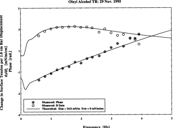
Oleyl alcohol was tested on several occasions to serve as a baseline for data comparison. After cleaning, the trough was filled with distilled water and one drop of oleyl alcohol, - 15 ylu, was applied to the surface. Due to the disparity in surface tension and density between water and oleyl alcohol the later is a self spreading compound. Excess droplets, when present, were wiped to the left end of the trough and contained behind a film barrier. In all cases the elastic properties measured before and after data collection adequately explained the dynamic behavior for frequencies up to 3 Hz. Data collected above 3 Hz showed considerable scatter. The scatter was due to the longitudinal wavemaker generating transverse waves in the direction of the longitudinal waves.

(29)

Oleyl Alcohol TR: 13 Aug. 1995

0 1 2 3 4

Frequency [Hz]

Figure 5.1 Variation in Surface Tension: Oleyl Alcohol y = 68.0 mN / m

Oleyl Alcohol TR: 29 Sept. 1995

Frequency [Hz]

Figure 5.2 Variation in Surface Tension: Oleyl Alcohol y = 67.0 mN / m

N U Cu I-Cu N C 0 CuS QCu .i. I.. Cu UE N N8 Cu

(30)

Oleyl Alcohol TR: 29 Nov. 1995

Frequency [Hz]

Figure 5.3 Variation in Surface Tension: Oleyl Alcohol y = 70.0 mN / m

Oleyl Alcohol TR: 29 Nov. 1995

0 1 2 3 4

Frequency [Hz]

Figure 5.4 Variation in Surface Tension: Oleyl Alcohol y = 70.0 mN / m

A z ME . A C z0 cc "g 5

(31)

Oleyl Alcohol TR: 3 Dec. 1995

Frequency [Hz]

Figure 5.5 Variation in Surface Tension: Oleyl Alcohol y = 69.0 mN / m

Oleyl Alcohol TR: 5 Dec. 1995

Frequency [Hz]

Figure 5.6 Variation in Surface Tension: Oleyl Alcohol y = 70.0 mN / m

U 0 I-C' .o C' a U C' I.- 3-C' C,~C

(32)

5.3. Analysis of Seawater Surfactants

5.3.1. Analysis of Cohasset Seawater

On several occasions, water was collected and analyzed from the inlet to Little Harbor near Cohasset Ma. Little Harbor is located on the northern shore of Cape Cod taking in water from the Bay of Massachusetts. Water was collected during daylight hours near the end of the flood tide. The shape of the inlet allows a large eddy to form during flood tide, concentrating surface surfactant when present.

After collection and transportation to the laboratory, seawater samples were placed in the Wave Decay Tank or, in the case of a smaller sample, a 50 liter holding tank equipped with surface skimming apparatus. The Longitudinal Wave Trough was filled with water skimmed off the larger tank. This process ensured an adequate supply of surfactant. In those cases where samples were tested for both wave decay properties and variations in surface tension, wave decay experiments were performed and surfactant was skimmed off the Wave Decay Tank. Prior to dynamic testing several pressure-area isotherms were measured to determine the quasi-static elasticity. Dynamic data is compared to theoretical predictions based on quasi-static elasticity measured following the dynamic tests

Cohasset Seawater TR: 14 Aug. 1995

N

*0I_6ý rA

Frequency [Hz]

(33)

Cohasset Seawater with Sodium Azide TR: 5 Sept. 1995 I U-s*p. *0 Frequency [Hz]

Figure 5.8 Variation in Surface Tension: Cohasset Seawater y = 68.0 mN / m

Cohasset Seawater TR: 5 Oct. 1995

AP'ur

Frequency [Hz]

(34)

5.3.2. Analysis of Woods Hole Seawater

Two water samples were collected from a salt pond on the south shore of Cape Cod fed by an inlet to Vineyard Sound. The first sample was collected from the inlet during ebb tide on the morning of November 18. Containers were lowered into the flow out of the inlet taking care not to disturb the material on the bottom or banks. Water was transferred from collection containers to 50 liter containers allowing 400 liters to be transferred to the Marine Instrumentation Laboratory MIT. Samples were stored overnight in the 50 liter transport containers and dynamic properties were measured on November 19. Upon completion of wave decay experiments seawater and surface films were transferred to the Longitudinal Wave Trough by skimming film off the surface of the Wave Decay Tank. Variations in surface tension were measured in the longitudinal wave trough at frequencies between 0.6 to 3.2 Hz. Variations in surface tension magnitude corresponded to predictions made from the quasi-static elastic properties. However, the measured phase relationship between the longitudinal wavemaker and variations in surface tension for low frequency deviated slightly from predicted values. The error in phase for 0.6 Hz represents variations in surface tension occurring 0.1 sec before predicted variations. The error may be due to a change in film properties due to its age but remains unexplainable without future experiments.

Woods Hole Seawater TR: 19 Nov. 1995

a as-p .

Frequency [Hz]

Figure 5.10 Variation in Surface Tension: Woods Hole Seawater y = 70.0 mN / m

The second sample was collected from the salt pond, concentrated using a centrifuge and eluted with methanol into a concentrate. Collection and concentration were carried out by

(35)

Robert Nelson of the Woods Hole Oceanographic Institute. The concentrate was spread onto tap water that had been wiped clean. A micro pipette was used to spread - 200 Pl of the concentrate on the water surface.

During concentrate spreading for the December 5 experiment several droplets of concentrate sank to the bottom of the trough. The droplets could not be moved from below

the laser apparatus resulting in difficulties maintaining a constant surface film pressure during the experiment. The variation in film pressure resulted in variations in elasticity and increased scatter during the experiment.

During concentrate spreading for the December 6 experiment care was taken to spread concentrate behind the longitudinal wavemaker in smaller quantities. Several small droplets sank but leakage was confined outside the test area. Data scatter was reduced and the dynamic behavior corresponds to predictions made from the quasi-static elasticity.

Woods Hole Methanol Concentrate TR: 5 Dec. 1995

2 3

Frequency [Hz]

(36)

Woods Hole Methanol Concentrate TR: 6 Dec. 1995 2 S a a a Ii-aa a Q J\ 0 1 2 3 4 5 Frequency [Hz]

Figure 5.12 Variation in Surface Tension: Woods Hole Concentrate = 70.0 mN / m

Woods Hole Methanol Concentrate TR: 6 Dec. 1995

Cu S a 0. U, a aB 0 a Cu" C,, Cu S a 0 1 2 3 4 5 Frequency [Hz]

(37)

5.4. Surface Viscosity Sensitivity Analysis

In an effort to quantify whether surface films possess significant surface viscosity, several test cases were run through the surface tension modeling program for a constant elasticity. Surface viscosity values ranging from 0.0 mN/m/sec to 1.0 mN/m/sec were used. The model predicts a significant reduction in the magnitude of surface tension variation with surface viscosity values greater than 0.1 mN/m/sec.

The phase relationship between the longitudinal wavemaker and variations in surface tension at the point where surface tension measurements are made is also affected by changes in surface viscosity. Varying surface viscosity shows changes in the phase relationship between wavemaker and measurement points for frequencies above 2 Hz and for surface viscosity values greater than 0.5 mN/m/sec.

Examination of the experiential data with respect to surface viscosity reveals that surface viscosity must be negligible in the films tested.

Variation in Surace Tension Magnitude to Surface Viscosity TR: 7 Dec. 1995

MJ i.. I-j rinc Cu~ Frequency [Hz]

Figure 5.14 Variation in Surface Tension Magnitude due to Surface Viscosity -Elasticity = 25.0 mNIm S. Viscosity = 1.0 mN/m/sec

- - - - Elasticity = 25.0 mN/m S. Viscosity = 0.5 mN/mn/sec

- - - - Elasticity = 25.0 mN/m S. Viscosity = 0.1 mN/m/sec

Elasticity = 25.0 mN/m S. Viscosity ' • • I = | 0.0 mN/m/sec, t I I

-i · · · ·

(38)

Variation in Surface Tension Phase to Surface Viscosity TR P6 E o a a td g-*aa U ag~I-e a 5) aP a Frequency [Hz]

Figure 5.15 Variation in Surface Tension Phase due to Surface Viscosity

.- - - Elasticity = 25.0 mN/m S. Viscosity = 0.1 mN/m/sec

-- -- Elasticity = 25.0 mN/m S. Viscosity = 1.0 mN/m/sec

- - - - Elasticity = 25.0 mN/m S. Viscosity = 0.5 mN/m/sec

---- Elasticity = 25.0 mN/m S. Viscosity = 0.0 mN/m/sec

(39)

6. Dynamic Properties of Surface Films: 4.0 to 24.0 Hz

The decay rate of transverse water waves propagating on a film covered surfaces were discussed in section 2.1. Using the Wave Decay Tank, described in Appendix B, we were able measure decay rates over a range of frequencies from 4.0 to 24.0 Hz.

6.1. Experimental Procedure

Procedure can be broken down into three areas; cleaning, setup and data collection.

6.1.1. Cleaning

Prior to testing great care must be taken to remove contaminants. The Wave Decay Tank was rinsed with tap water and dried using a vacuum squeegee. The wavemaker, beach and skimmers were washed with tap water and dried using solvent free paper wipes.

Prior to testing decay rates of clean water and spread films on tap water the surface was "wiped" clean or skimmed to remove any contaminants. Two film barriers were constructed to slide on the tank walls. The barriers pierced the air-water interface with seals along the tank walls. Sliding the barriers along the tank trapped and compressed contaminants to the point where they could be vacuumed off.

6.1.2. Setup

Two types of underlying fluid were tested in the wave decay tank. The first, tap water, was used during the measurement of clean water decay and as a base for spread films. After cleaning, the tank was filled with tap water through a garden hose to a depth of 10 cm. The water was left to stand for 20 minutes and the surface was skimmed. After skimming, cleanliness was ensured by measuring the surface tension of and comparing it to typical values for clean water.

Two types of tests were conducted using tap water as a base. Decay tests were performed checking clean water decay rates. The clean water decay rates served as a baseline check testing the apparatus for repeatability. Upon completion of successful clean water decay tests, surfactant was spread on the tap water surface. Two spread films were tested, oleyl alcohol and Woods Hole seawater concentrate.

Seawater was the second base fluid. The tank was cleaned with tap water and filled with seawater that had been transported to the laboratory from site collection. Once filled to a depth of 10 cm the water was left to stabilize for '/2 hour. In the event more surfactant was needed a smaller tank equipped with a skimming apparatus was filled with seawater and surface surfactant was skimmed into a 200 ml beaker and transferred to the Wave Decay Tank.

Several pieces of equipment were shared between the wave decay experiments and the variation in surface tension experiments. Moving from one experiment to the other required

(40)

relocating the electronic balance and reconfiguring the data processing and collection equipment.

6.1.3. Data Collection

Data collection was done in three steps. 1) Pressure-Area Isotherm. 2) Decay Data and 3) Pressure-Area Isotherm. The isotherm data was collected by submerging the beach, placing a film barrier at the "0" location and using a second film barrier to compress the surface film. After the pressure-area isotherm was completed the film pressure was adjusted to -2mN/m by moving the film barrier, the beach was raised into position, and the transverse wavemaker was installed. Decay data collection started with a frequency of 4 Hz and then was done at progressively higher frequencies. The electronic balance and Wilhelmy Plate were located forward of the beach and kept in contact with the water during decay data collection ensuring continuous monitoring of film pressure.

6.2. Measured Decay Rates of Clean Water

Clean water was used as a baseline checking the test apparatus and data reduction software. The tank was filled with MIT tap water to a depth of 10 cm. The surface was wiped clean by removing any surfactants from the surface area of interest.

Transverse wave decay was measured over frequencies ranging from 4 to 30 Hz. In all cases the decay rates matched those predicted by equation 2.24.

Clean Water WDT: 02 Oct. 1995

0.10

ca

cc

0.05

Frequency [Hz]

Figure 6.1 Transverse Wave Decay Rates: Clean Water y = 72.0 mN / m

0 Measured Data

- Theoretical Clean Water Decay

-o - _ p_.

c 0

--11 11

(41)

Clean Water WDT: 04 Oct. 1995

0.10

0.05

Frequency [Hz]

Figure 6.2 Transverse Wave Decay Rates: Clean Water y = 72.0 mN / m

Skimmed Tap Water WDT: 07 Dec. 1995

0.10

S 0.05

Frequency [Hz]

Figure 6.3 Transverse Wave Decay Rates: Clean Water y = 72.0 mN / m

41

0 Measured Data

- -- Theoretical Clean Water Decay

--C

---

-O Measured Data

- -- - Theoretical Clean Water Decay

..0.•. - -• ' ' '

11

Dynamic properties of seawater surfactants

Dynamic Properties of Seawater Surfactants

FEB 2 0

1997

Dynamic Properties of Seawater Surfactants

by

ACKNOWLEDGMENTS

TABLE OF CONTENTS

LIST OF FIGURES

LIST OF SYMBOLS

k

1. Introduction

2. Theory

= 4ei(kx-a)

(2.1b)

(pw

-

-pgkf) = 0

(2.8)

(2.5)

0

0

(2.16)

=

e

+

Ae

e

e

[

+

(2.21)

y'

=

eikLX

(2.22)

(p

-

- pgk) =

O

(2.5)

3. Apparatus

i/

/I

K

I~j

LIr

r`

4. Experiments and Results

5. Dynamic Properties of Surface Films:

0.5

to 4.0 Hz

6. Dynamic Properties of Surface Films: 4.0 to 24.0 Hz

ca

cc

_-

_{-pgkf) = 0}

_-

_{- pgk) =}

_O

_(2.5)