HAL Id: hal-00316943
https://hal.archives-ouvertes.fr/hal-00316943
Submitted on 1 Jan 2002
HAL is a multi-disciplinary open access
archive for the deposit and dissemination of
sci-entific research documents, whether they are
pub-lished or not. The documents may come from
teaching and research institutions in France or
abroad, or from public or private research centers.
L’archive ouverte pluridisciplinaire HAL, est
destinée au dépôt et à la diffusion de documents
scientifiques de niveau recherche, publiés ou non,
émanant des établissements d’enseignement et de
recherche français ou étrangers, des laboratoires
publics ou privés.
Estonian total ozone climatology
K. Eerme, U. Veismann, R. Koppel
To cite this version:
K. Eerme, U. Veismann, R. Koppel. Estonian total ozone climatology. Annales Geophysicae, European
Geosciences Union, 2002, 20 (2), pp.247-255. �hal-00316943�
Geophysicae
Estonian total ozone climatology
K. Eerme, U. Veismann, and R. Koppel
Tartu Observatory, T˜oravere, 61602, Tartumaa, Estonia
Received: 16 November 2000 – Revised: 20 July 2001 – Accepted: 3 October 2001
Abstract. The climatological characteristics of total ozone
over Estonia based on the Total Ozone Mapping Spectrome-ter (TOMS) data are discussed. The mean annual cycle dur-ing 1979–2000 for the site at 58.3◦N and 26.5◦E is com-piled. The available ground-level data interpolated before TOMS, have been used for trend detection. During the last two decades, the quasi-biennial oscillation (QBO) corrected systematic decrease of total ozone from February–April was 3 ± 2.6% per decade. Before 1980, a spring decrease was not detectable. No decreasing trend was found in either the late autumn ozone minimum or in the summer total ozone. The QBO related signal in the spring total ozone has an ampli-tude of ± 20 DU and phase lag of 20 months. Between 1987– 1992, the lagged covariance between the Singapore wind and the studied total ozone was weak. The spring (April–May) and summer (June–August) total ozone have the best correla-tion (coefficient 0.7) in the yearly cycle. The correlacorrela-tion be-tween the May and August total ozone is higher than the one between the other summer months. Seasonal power spec-tra of the total ozone variance show preferred periods with an over 95% significance level. Since 1986, during the win-ter/spring, the contribution period of 32 days prevails instead of the earlier dominating 26 days. The spectral densities of the periods from 4 days to 2 weeks exhibit high interannual variability.
Key words. Atmospheric composition and structure (middle
atmosphere – composition and chemistry; volcanic effects) – Meteorology and atmospheric dynamics (climatology)
1 Introduction
Harmful effects of solar UV-B radiation on humans and other biospheric species necessitate retrospective studies of UV climatologies, which focus on the factors affecting the ground-level UV irradiance and deal with their statistical characteristics, such as mean values, variability and trends.
Correspondence to: K. Eerme ([email protected])
The present paper concentrates on the study of available total ozone data over one geographical site that can be considered representative of the entire Estonia.
The mean annual cycle of atmospheric total ozone over middle and high-latitudes is believed to be transport-governed (Randel et al., 1993; Chipperfield and Jones, 1999; Rosenlof, 1999), exhibiting high values in late winter and spring (February–April) and the lowest values during late autumn (October–November). The year-to-year changes in the annual transport cycle depend on the changing planetary wave activity (Kinnersley, 1998) which is connected to the QBO (Tung and Yang, 1994a, b; Yang and Tung, 1995; Hol-landsworth et al., 1995; Kane et al., 1998).
The variance around the annual cycle contains different contributions of shorter scale variations that vary with the geographical region. Globally, fourteen of the most contigu-ous subregions have been identified, each displaying statis-tically unique total ozone variability characteristics (Eder et al., 1999). Estonia is located between the North Atlantic, and the Eurasian and is influenced more by the baric situation over the North Atlantic, and manifests a comparatively high contribution of synoptic-scale variation in the total ozone variance. Strong planetary wave activity in the winter-spring causes low total ozone values over northern Europe (Engelen, 1996). During the early spring, some influence of ozone-depleted stratospheric air, eroded from the polar vortex, is possible (Knudsen and Grooß, 2000).
The chemical destruction of ozone by stratospheric sul-phate aerosol outside the vortex can be enhanced by the stratospheric cooling (McCormick et al., 1995) and the in-crease in the halogen species burden. Since 1978, two ma-jor and several minor volcanic eruptions have contributed to the stratospheric aerosol surface area which had been much higher in background level in 1982–1983, 1992–1994 and to a lesser extent in 1980 and 1985–1988 (Solomon et al., 1996).
In the short-term variability, the high total ozone events ap-pear when the geopotential heights of the upper tropospheric pressure levels (500 hPa, 300 hPa) are low, and the low
to-248 K. Eerme et al.: Estonian total ozone climatology
Fig. 1. Annual mean cycle of total ozone over Estonia 1979–2000
based on TOMS averaged ten-day values, (1983, 1992 and 1993 excluded).
tal ozone events appear when these geopotential heights are high. Another source of short-term variability of total ozone is the filamentation of stratospheric air related to the subtrop-ical barrier and the wintertime polar vortex, both of which isolate the air inside by strong winds. The breaking of plan-etary waves in the stratosphere over latitudes close to the subtropics results in the activity of filamentation (Morgen-stern and Carver, 1999), exhibiting a large temporal variabil-ity on time scales of days to weeks. Favorable breaking of Rossby waves near the end of the North Atlantic storm track induces increased filamentation in that region. The frequency of laminae over central Europe was observed to be five times higher in late winter to early spring than in autumn (Mlch and La˘stovi˘cka, 1996), and exhibits a maximum in March and minimum during July to October (Reid et al., 2000). Dur-ing the existence of the polar vortex, the laminae can form in the region of the vortex edge. Above approximately 16 km, the air deep inside the vortex is essentially isolated from the extra vortical air, but the air in the vortex edge is sporadi-cally transported to the middle and low-latitudes (Waugh et al., 1997).
2 Total ozone data sources
Regular direct Sun total ozone measurements in Estonia (at T˜oravere, 58.3◦N, 26.5◦E, 70 m above sea level) have been carried out since January 1994, using the laboratory spec-trometer SDL-1 supplied with a mirror system and Dob-son retrieval algorithm (Veismann et al., 1995; Eerme et al., 1998). Regular measurements of the erythemally weighted UV irradiance at the same site have been performed since 1 January 1998 (Veismann et al., 2000). Direct Sun measure-ments of total ozone have been possible during about one-third of the days since March to October and available only in a very few cases during the winter months. For climato-logical studies, a longer record and more dense time cover-age are necessary. The available total ozone, data extending back to November 1978, are those from the Nimbus-7 Total Ozone Mapping Spectrometer TOMS (until May 1993) and
Fig. 2. Examples of frequency distributions of total ozone
deriva-tions from the long-term mean (a) in the summer seasons and (b) in the winter/spring seasons .
other TOMS (http://jwocky.gsfc.nasa.gov/) or TIROS Oper-ational Vertical Sounder TOVS instruments. The most ho-mogeneous data set comes from the Nimbus-7 TOMS. Since July 1996, the available Earth Probe TOMS data have been regularly compared to the ground-level measurement data obtained at T˜oravere. The correlation coefficient between both values was found to be between 0.92 and 0.97 in dif-ferent years. The best agreement appeared in 1999 when the mean ratio of 124 compared values TOMS/T˜oravere was 0.998 with the standard deviation of 0.031. The largest dif-ferences in this year did not exceed ± 10%. During 1996– 1998, the TOMS mean values systematically were about 7% lower than our ground-level values, and 96% of the values were within ± 10% of this mean. The standard deviations
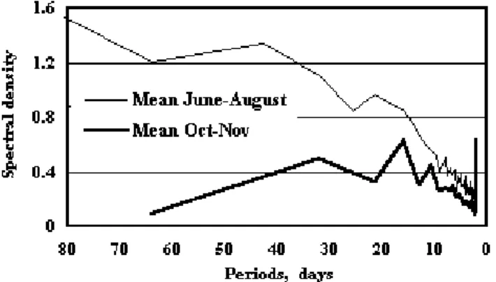
Fig. 3. Mean power spectra of total ozone deviations for the summer
season (June–Aug.) and the late fall minimum (Oct.–Nov.) 1979– 2000.
of the ratios TOMS/T˜oravere in these years were between 5 and 7%. In a few cases, the differences between both values reached ± 20%. The Meteor-3 total ozone data, containing plenty of longer or shorter gaps, can be used with some cau-tion only for the calculacau-tion of the seasonal mean, but not for calculating power spectra. The differences between the Nimbus-7 and Meteor-3 TOMS values rarely exceeded 10 DU. No TOMS data are available between November 1994 to August 1996.
During the pre-TOMS time, a coarse picture about the total ozone variation can be obtained, using the averaged global distribution data of the ground-based network, oper-ating since 1957. The published gridded data of monthly mean total ozone are available for the first ten years (1957–1967)(London et al., 1976). The monthly mean values of operating ozone stations can be found on the WMO World Ozone and Ultraviolet Data Center homepage (http://www.tor.ec.gc.ca/woudc). For our site, the values can be interpolated in the best way by using the St. Petersburg and Riga data. For both stations, no data are available from 1968 to 1972.
In addition to trend detection, the background normal ozone levels, including both the mean value and the mean variance in different time scales, are necessary for the study of the total ozone anomalies. The major governing processes of the total ozone variation, such as Rossby wave positions, the upper tropospheric pressure pattern and the preferred re-gions of filament movements, create unique conditions even for quite, small geographical regions that require their own ozone climatologies.
3 Mean annual cycle
A mean annual cycle of total ozone over Estonia between 1979–2000, composed using the averaged ten-day values, is presented in Fig. 1, as well as the standard deviation limits and the ten-day extreme values. The years subjected to strong stochastic forcing by El Chichon (1983) and Mt. Pinatubo
Fig. 4. Mean winter/spring power spectra of total ozone deviations
for 1979–1985 and 1986–2000.
(1992 and 1993) volcanic aerosol are excluded, since they contain anomalously high amounts of low total ozone (Bo-jkov, 1993). Due to the gap in the data set used, the year 1995 and part of 1996 have also been excluded. Post-volcanic low values of total ozone are systematically met from January to September. To a lesser extent, the summer total ozone is affected. No volcanic influence was noticed during the late autumn total ozone minimum.
The main characteristics of the annual and interannual variability of the total ozone over Estonia, including the post volcanic years of 1983, 1992 and 1993, are presented in Table 1. The first three columns present the monthly ab-solute maximum, the mean with ± standard deviation (σ ) limits, and the absolute minimum values. The next three columns present the maximum, mean ±σ and minimum of the monthly amplitudes of the total ozone variation. The last column presents the amplitude of the differences in the yearly monthly mean values. This amplitude exceeds 100 DU from February to April, and reaches the lowest values of about 40 DU from September to November. The higher amplitude 50 DU in October is due to the contribution of the extremely low mean in 1989. The comparatively high amplitude for August originates from the extremely high mean value in 1998.
The linearly approximated decrease in the mean total ozone from the middle of April to the second half of Septem-ber was found to be 19.5 DU per month. During the two autumn months from October to November, the mean to-tal ozone remains almost at the persistent and lowest level of around 288 DU. In December, it usually increases sharply and persists at the level of about 340 DU from late December to the end of January. At that time, significant year-to-year and yearly variations take place. The highest daily values of mean total ozone occurred from February to April, as well as the highest day-to-day differences.
250 K. Eerme et al.: Estonian total ozone climatology
Table 1. Some characteristics of total ozone variation over Estonia, based on TOMS data, November 1978–December 1999
Month Total zone, DU Amplitude of yearly Difference of monthly variation, DU mean, DU
Max Mean Min Max Mean Min
Jan. 473 337 190 261 145 104 87 Feb. 533 368 192 340 182 102 111 Mar. 517 390 244 232 165 119 107 Apr. 507 395 281 181 136 90 100 May 486 375 295 143 104 50 65 Jun. 430 355 297 117 77 42 49 Jul. 402 340 288 103 74 48 45 Aug. 388 321 262 96 70 50 59 Sep. 367 300 233 125 84 50 38 Oct. 378 289 218 128 95 65 50 Nov. 409 288 204 161 106 75 39 Dec. 440 316 208 193 141 68 73 4 Short-term variability
The probability distributions and the power spectra of the ob-served total ozone deviations from the long-term mean were calculated for different seasons. For the summer season, the long-term mean was approximated as linearly decreas-ing from 11 May to 15 September (allowdecreas-ing for 128 values). The σ values of the total ozone variations in the observed summers occurred between 18.7 and 27.5 DU (the lowest in 2000 and the highest in 1998). In more than half of the cases,
σwas within the limits of 20–22 DU. The winter/spring sea-son was from 1 January to 7 May, thus the long-term mean was smoothly interpolated. The yearly values of σ were be-tween 35 and 54 DU, with the lowest in 1993 and the highest in 1989. For the long-term mean from October–November, a constant value of 288 DU was taken and 64 points for the Fourier transform were used from 28 September to 30 November.
The typical amplitude of the deviations from the mean was around ± 50 DU in the summer season, and around
±100 DU in the winter/spring season. Often there are met peaks on both sides of the central maximum of the proba-bility density distribution of the total ozone deviations, cor-responding to the upper tropospheric highs and lows. The central mode is stronger since for most of time, Estonia is located under transition conditions between the upper tropo-spheric high ridges and the troughs. The examples of dis-tributions for the summer and winter/spring seasons are pre-sented in Fig. 2. In the post-volcanic years of 1983, 1992 and 1993, the winter/spring means dropped below the long-term mean by 15, 26 and 46 DU, respectively. The summer mean in 1983 and in 1992 was lower by 17 DU. In the summer of 1993, there was a gap of data exceeding one month in June and July. In the volcanically nondisturbed years, the differ-ences in the annual seasonal mean from the long-term mean
were between −9 DU and +13 DU in the summer and be-tween −14 DU and +22 DU in the winter/spring. Negative and positive skewness values in the probability density distri-butions of the total ozone deviations were found with almost an equal frequency. The negative kurtosis values dominated slightly (58%) in the summer and the positive values domi-nated to the same extent in the winter and autumn.
The power spectra of the total ozone deviations from the long-term mean display peaks at certain frequencies. The mean spectra in the period scale for the summer and autumn seasons are presented in Fig. 3. In late autumn, spectral den-sities that exceed the 95% significance above the background appear regularly at periods of 16 and 10 days. Additionally, a peak on the 90% significance level appears at a period of 32 days. In summer, the most prominent peaks of the 95% significance are around 43 and 21 days. The spectral densi-ties in shorter periods within the interval from 4 days to two weeks show high interannual variability and each of them has a small contribution to the mean spectrum.
In winter, the spectral densities above the 95% significance level were met within the periods of 26 days, and 13 to 16 days before 1986. Later, the contributions of the periods of 32 days and 18 to 21 days became more prominent. The mean spectra for the intervals between 1979–1985 and 1986– 2000 are presented in Fig. 4 and the typical representatives of spectra from both intervals of the winter/spring spectra in 1981 and 1990 are presented in Fig. 5.
It should be noted that the interval of 1986–2000 consists of two isolated subintervals, and the year-to-year variations of the meteorological conditions during both have been pri-marily higher than during the beginning part of the TOMS total ozone record. The conditions in the very last years of the observed period have been discussed in several recent pa-pers. An extremely long-lived vortex, centered primarily at
Fig. 5. Examples of typical winter/spring power spectra of total
ozone deviations from the intervals 1979–1985 (1981) and 1986– 2000 (1990).
the pole, was observed during the winter of 1996/97 (Hansen and Chipperfield, 1999). Relatively low values of total ozone in the lower stratosphere that winter were related to an in-creased filamentation from the subtropical barrier. About 30% more filaments were found in January–February 1997 than in 1998 (Morgenstern and Carver, 1999). An atypically early major stratospheric warming in December 1998 re-sulted in an abnormally warm and weak polar vortex through most of the 1998/99 winter (Manney et al., 1999) and in the high total ozone.
The detected modes of temporal variability in the total ozone should reflect the multiscale circulation modes of the atmosphere that modulate the geopotential height. In the study of global, multiscale, low-frequency circulation modes (Lau et al., 1994) the pronounced peaks of variation at about 40–60 days and 20–30 days in the North Atlantic/Eurasian area were found. By Yan et al. (2001) the principal time scale of a weather change for about 16 days in Europe was found on the basis of the Swedish and St. Petersburg long-term data. May (2000) performed a study of the atmospheric intraseasonal variability with the aim of finding the contri-butions of the ultra-long, long and short planetary waves in the 500 hPa geopotential height variance. As the contribu-tion of the longer waves dominates, the spectral density is the highest at periods of about 20 days. The adequate ex-planation of the detected periods in the Estonian total ozone variance requires more detailed study currently under way of the geopotential height variance, as well as the upper tropo-spheric pressure.
5 QBO-related variations
The global total ozone data measured by Nimbus-7 TOMS in the different latitudinal belts have been studied in several cases (Tung and Yang, 1994a; Yang and Tung, 1995; Hol-landsworth et al., 1995; Kane et al., 1998). Maximum cor-relation of the total ozone with the 30 hPa equatorial zonal
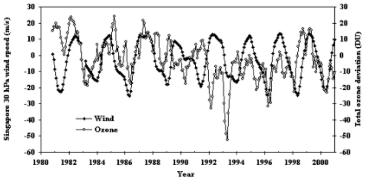
Fig. 6. Covariance of T˜oravere total ozone deviations (DU), lagged
by 20 months of the Singapore 30 hPa wind speed (m/s).
wind, at almost a zero lag or a wind lead of 1–2 months, was found over the equator. The QBO in the extratropical ozone was found by Yang and Tung (1995) to be seasonally synchronized with the strong signal in the winter-spring sea-son out of phase with the equatorial ozone. The dynamical explanation of the influence of QBO on the diabatic mean meridional circulation is given by Tung and Yang (1994b). The anomaly in the circulation is responsible for the merid-ional transporting of the ozone to create an anomaly in its column and, therefore, a phase lag in the ozone anomaly can expected.
We compared the four month moving average of the cur-rent deseasonalized monthly mean total ozone anomalies (deviations of current monthly mean values from the long-term monthly mean) with the 30 hPa stratospheric zonal wind speed at Singapore. The best covariance in phase for the pe-riod of 1979–2000, covering 9 QBO wind cycles, was found in the case of the phase lag of the total ozone for 19 to 20 months. The 20-month lagged covariance of the total ozone with the Singapore 30 hPa zonal wind speed (westerlies were positive) is presented in Fig. 6. Both the prominent maxima and minima in the total ozone appeared to be strong in the winter-spring. The phase lag during the 1980’s tended to be about one month longer than during the last three QBO wind cycles in the 1990’s. The cycles corresponding to the wester-lies’ maxima in November 1987 and August 1990 exhibited a worse covariance than the remaining cycles.
6 Observed trends
The studies of the total ozone trends have quite a long history. According to recent estimations, the linear downward trend of total ozone over the northern mid-latitudes of 50◦–65◦ since 1979 has been 4.4 ± 2.6% per decade for December– May and 2.8 ±1.3% per decade for June–November (WMO, 1998) with the uncertainty level of 2σ . Here, we tried to de-tect the seasonal trends for a longer time interval, including the monthly mean data of 1957–1967 (London et al., 1976) and the interpolated monthly mean values from the Riga and St. Petersburg stations data in 1973–1978. The results are presented in Fig. 7. As representative of the ozone transport minimum, we took the mean value of the two autumn months
252 K. Eerme et al.: Estonian total ozone climatology
Table 2. Yearly numbers of low and high ozone days
Low ozone days High ozone days
Mean- Mean + Low + high
Mean −σ
2σ Mean +σ 2σ ozone days
Year
Total Feb.–Apr. Jun.–Aug. Total Total Feb.–Apr. Jun.–Aug. Total over ± 1 σ
1979 30 0 7 5 87 23 25 17 117 1980 15 7 3 0 107 15 29 18 122 1981 43 6 16 2 73 27 9 20 116 1982 39 11 7 4 74 27 26 4 113 1983 92 19 32 8 34 7 6 3 126 1984 49 13 13 1 61 13 17 9 110 1985 50 3 26 9 60 18 8 5 110 1986 67 27 24 4 44 7 7 5 111 1987 29 7 6 3 78 25 24 7 107 1988 57 5 18 6 49 18 14 10 106 1989 66 8 22 5 37 18 6 7 103 1990 68 21 17 6 44 7 8 5 112 1991 47 8 16 1 69 11 22 11 116 1992 114 19 34 16 21 10 4 2 135 1993 37 >12 0 1994 11 19 3 1995 1996 1997 97 30 16 4 41 15 2 4 138 1998 49 17 5 3 81 11 37 17 130 1999 55 4 20 0 53 19 2 4 108 2000 85 31 12 12 18 4 7 1 103 Mean 58.5 14.2 16.5 5.3 57.5 13.9 14 8.3 116
(October and November). In the ten-day means within these two months, the values above the mean for a whole period have prevailed slightly (54%) since 1979. During most years, the ten-day mean deviations, with plus and minus signs occur in the following proportions: 3:3 or 4:2. Approximately the same was found in the case of the three summer months from June to August. The estimated linear trends for October– November and for June–August with error limits ±2σ were
−0.2 ± 2.8% and +0.05 ± 2.9%, respectively, per decade. The value of σ was estimated, taking into account the auto-correlation, as proposed by Kadygrova and Fioletov (1987). Due to the rather large intrinsic noisiness of the data, no trend can be detected in summer months or in the autumn ozone minimum.
A mean value of three months (February to April) was taken as representative of trend calculations for the winter ozone transport maximum since the transport peaks at differ-ent times in differdiffer-ent years, and often the peak is masked by synoptic frequency variations in the total ozone. The nois-iness of the data is larger than in the previous two cases, including the QBO-related variations. The three month
av-eraged values during the 1980’s and the 1990’s tend to be lower than before. It is suspected that the downward trend in the winter/spring total ozone began only at about 1980. The estimated trend before 1980 was 0.6 ± 5.2%, and after 1980, it was −3.0 ± 3.7% per decade. An attempt was made to remove the QBO signal in the February to April yearly mean total ozone, thus correcting it for the half-amplitude in the cases with lagged total ozone corresponding to the Singa-pore wind maxima and minima. The SingaSinga-pore 30 hPa wind cycles and interpolated total ozone data for 1958–1967 and since 1973 were taken into account. When the lagged min-ima or maxmin-ima occurred during the other seasons and did not notably affect the spring total ozone, no correction was made. The spring seasons of 1983, 1992 and 1993, where the total ozone was strongly influenced by volcanic aerosol, were ex-cluded. After this correction, the noisiness of the data for trend calculation was reduced to some extent. The calculated trend in 1980–2000 was 3.0 ± 2.6%, instead of −3.0 ± 3.7% before the correction.
Indirect evidence of the decreasing trend of the total ozone in late winter and early spring can be found by comparing
Fig. 7. Trend lines of total ozone X 1958–2000: t – years from
1958; 1 – winter/spring (Feb.–Apr.), 2 – summer (June–Aug.), 3 – late autumn (Oct.–Nov.).
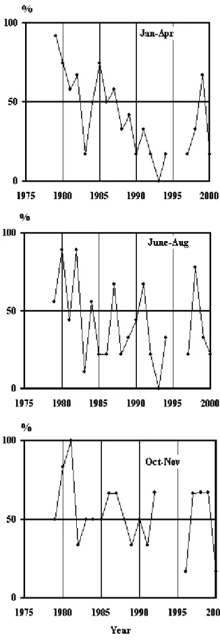
the deviations of the observed total ozone from the mean of 1979–2000. The variations in the yearly percent of positive deviations for the ten-day means from the long-term mean for the periods of January–April, as well as for June–August and October–November, are presented in Fig. 8. In the January– April ten-day mean total ozone values during 1979–1987 the values were higher when the long-term mean prevailed, ex-cept during the post-volcanic year of 1983. Since 1988, the total ozone values below the long-term mean have domi-nated, except for the year 1999, where the values were simi-lar to those in the early 1980’s and corresponded to the QBO-related total ozone maximum. The other QBO-QBO-related peaks appear before 1990, in the winter-spring periods of 1979, 1982, 1985, 1987 and 1989. The QBO-related minima ap-pearing in 1981, 1984, 1986 and 1998 are less pronounced. The ten-day mean total ozone values below the long-term mean were dominant in the years after the major volcanic eruptions in the winter-spring as well as in the summer. The late autumn ten-day mean total ozone values do not manifest a volcanic or QBO influence.
If the mean total ozone during some time interval is lower or higher than the long-term mean, then with respect to the daily values, the same can be expected. Here, the days with total ozone values less than the long-term ten-day mean mi-nus σ are viewed as low ozone days, and the days with to-tal ozone higher than the long-term ten-day mean plus σ are viewed as high ozone days. Usually, only the deviations ex-ceeding ±2σ are considered as extremes. In deseasonalized total ozone variations, those extremes manifest a rather spo-radic nature. The total number of the high and low extremes varies between 4 and 22 days per year (the mean number 14 days). On average, the daily total ozone value exceeds ±σ in
Fig. 8. Percent of positive deviations of the yearly ten-day mean
values of total ozone from the long-term mean in the different sea-sons.
254 K. Eerme et al.: Estonian total ozone climatology
116 days per year (58.5 below and 57.5 above), and 8 to 10 days per month. Since 1979, a tendency to increase the lower and decrease the higher total ozone values is evident. The yearly numbers of low and high ozone days and both the ex-tremes are presented in Table 2, as well as the number of low and high ozone days in the winter/spring (February–April) and the summer (June–August). In the post-volcanic years of 1992 and 1983, the numbers of low ozone days were 114 and 92. Since 1986, large numbers of low ozone days tend to occur more often. The number 97 in 1997 even exceeded the value of post-volcanic 1983, and the number 85 in 2000 was also close. In 1998, containing the QBO-related total ozone spring minimum, the number of high ozone days in the sum-mer was the highest due to the dominating tropospheric low pressure. In most cases, the spring numbers of high ozone days tend to be larger in years containing the QBO-related spring total ozone maxima. A major contribution to the large number of low ozone days in the post-volcanic years comes from the summer months. From late September to Febru-ary, the very low ozone events, related to the advection of subtropical stratospheric air masses from the Azores’ anticy-clone to the northeast (Bekoryukov et al., 1994) are met in 2 to 7 cases in a year. A coincidence of the high upper tropo-spheric pressure and the filaments of ozone-poor air can lead to extremely low total ozone.
In different years since 1987, low ozone events have been recorded in late April and early May (in 1987, 1990, 1993, 1995 and 1997). The deepest low ozone events which ex-ceeded mean-2σ (295 DU) were in 1993 and 1997, and close to that time also (307 DU) in 1990 and 1995. The low ozone event over northern Europe in April 1997 has been discussed in detail by Austin et al. (1999). During this event, low ozone persisted over Estonia for 4 days, from 29 April to 2 May, and the UV exposures could reach the mid-summer levels.
The summer (June–August) mean total ozone is statisti-cally related to the spring (April–May) mean total ozone. The coefficient of linear correlation in 1979–2000 was 0.69 ± 0.12. On the level of the total ozone monthly mean values from April to August, a relatively high correlation was observed between May and August (0.73 ± 0.11) in 1979– 2000. The correlation coefficients between June, July and August as well as between May and June, and between May and July, the mean total ozone values were between 0.35 ± 0.12 and 0.50 ± 0.11. The correlation coefficient be-tween the April and May mean values was only 0.34 ± 0.13.
7 Summary and conclusions
The mean annual cycle of total ozone for one geographical site (T˜oravere, Estonia, 58.3◦N, 26.5◦E) is compiled based on Nimbus-7, Meteor-3, and Earth Probe TOMS data. The seasonal probability density distributions of the total ozone deviations from the long-term mean reveal, in most cases, additional maxima on both sides of the central maximum, corresponding to the synoptic-scale high and low pressure extremes in the upper troposphere. This exhibits the
con-tribution of non-stochastic processes in the total ozone vari-ance. The yearly mean standard deviations of the seasonal total ozone occurred between 19.5 and 27 DU in the sum-mer season and between 35 and 54 DU in the winter/spring season.
The power spectra of the total ozone deviations from the long-term mean exhibit spectral densities exceeding a 95% significance level over certain periods. In the summer, those periods are around 3 and 6 weeks. The contributions of peri-ods shorter than 2 weeks exhibit high interannual variability and do not contribute to the averaged spectrum. In the winter before 1986, the contributions of periods of 26 days and, 13 to 16 days were dominant instead of the periods of 32 days, and 18 to 21 days afterwards.
The amplitude of the QBO-related signal in the spring total ozone was around ± 20 DU. The phase lag with re-gard to the Singapore wind cycle was 19 to 20 months. a weak, lagging covariance with total ozone was noticed dur-ing two QBO wind cycles between 1987–1992. In the sum-mer, the QBO-like signal in the total ozone was found in single cases. In the autumn total ozone transport minimum (October–November), the manifestation of QBO and the in-fluence of major volcanic eruptions were not detected. In the years after the major volcanic eruptions, low values of mean total ozone were recorded in the spring and summer. In the post-volcanic summer seasons, the number of days with total ozone below mean σ exhibited record high values.
Due to high noisiness in the seasonally averaged total ozone, systematic trends above the 95% significance level cannot be detected in late autumn (October–November) or in summer (June–August) and late winter/spring, before 1980. In 1979–2000, the QBO corrected decreasing trend in late winter/spring (February–April) was found to be 3.0 ± 2.6% per decade within ± 2 s limits. The number of days with total ozone values lower than the mean minus the standard devia-tion has a tendency to increase. The values occurring above the mean in the years that were not volcanically disturbed were found only after 1986, with the highest value recorded in 1997. The extremely high yearly numbers of such low ozone days in the post-volcanic years of 1983 and 1992 con-tain relatively high contributions in the summer months.
Since 1979, a tendency to increase the lower and decrease the higher total ozone values is evident. Since 1986, large numbers of low ozone days tend to occur more often.
The summer total ozone is statistically related to the late spring total ozone level. The correlation coefficient between the mean total ozone of April–May and June–August in 1979–2000 was 0.69 ± 0.12. The dynamical and possibly the chemical changes in the total ozone before April do not influ-ence the summer total ozone, since the correlation was found to be below the significance level.
On the level of the monthly mean total ozone, the corre-lation in 1979–2000 was the highest (0.73 ± 0.11) between the May and August values. The correlation coefficients be-tween the June, July and August and bebe-tween April and May mean values were lower than 0.5.
Acknowledgements. The work was supported by the research grant 3609 of the Estonian Science Foundation. The authors would like to thank an anonymous reviewer for their constructive comments and suggestions.
Topical Editor D. Murtagh thanks a referee for his help in evalu-ating this paper.
References
Austin, J., Driscoll, C. M. H., Farmer, S. F. C., and Molyneux, M. J.: Late spring ultraviolet levels over the United Kingdom and the link to ozone, Ann. Geophysicae, 17, 1199–1209, 1999. Bekoryukov, V. I., Borisov, Yu. A., Zvyagintsev, A. M.,
Kruchenit-sky, G. M., Perov, S. P., and Rudakov,V. V.: Observations of two ozone “mini-holes” over Europe in early winter of 1992–1993, Izv. AN. Fizika atmosfery i okeana, 30, 807–811, 1994. Bojkov. R.: Record low total ozone during northern winters of 1992
and 1993, Geophys. Res. Lett., 20, 1351–1354, 1993.
Chipperfield, M. P. and Jones, R. L.: Relative influence of atmo-spheric chemistry and transport on Arctic ozone trends, Nature, 400, 551–554. 1999.
Engelen, R. J.: The effect of planetary waves on the total ozone deviations in the presence of a persistent blocking anticyclone system, J. Geophys. Res., 101, 28, 775–784, 1996.
Eder, B. K., LeDuc, S. K., and Sikkles, II, J. E.: A climatology of total ozone mapping spectrometer data using rotated principal component analysis, J. Geophys. Res., 104, 3691–3709, 1999. Eerme, K., Veismann, U., Koppel, R., and Pehk, M.: First four
years of atmospheric total ozone measurements in Estonia, Proc. Estonian Acad. Sci. Biol. Ecol., 47, 188–202, 1998.
Hansen, G. and Chipperfield, M. P.: Ozone depletion at the edge of the Arctic polar vortex 1996/1997, J. Geophys. Res., 104, 1837– 1846, 1999.
Hollandsworth, S. M., Bowman, K. P., and McPeters, R. D.: Obser-vational study of the quasi-biennial oscillation in ozone, J. Geo-phys. Res., 100, 7347–7361, 1995.
Kadygrova, T. V. and Fioletov, V. E.: Estimation of statistical char-acteristics of total ozone content, Soviet Meteorology and Hy-drology, 12, 29–43, 1987.
Kane, R. P., Sahai, Y., and Casiccia, C.: Latitude dependence of the quasi-biennial oscillation characteristics of total ozone measured by TOMS, J. Geophys. Res., 103, 8477–8490, 1998.
Kinnersley, J. S.: Interannual variability of stratospheric zonal wind forced by the northern lower stratospheric large-scale waves, J. Atmos. Sci., 55, 2270–2283, 1998.
Knudsen, B. M. and Grooß, J.-U.: Northern midlatitude strato-spheric ozone dilution in spring modeled with simulated mixing, J. Geophys. Res., 105, 6885–6890, 2000.
Lau, K.-M., Sheu, P.-J., and Kang, I.-S.: Multiscale low-frequency circulation modes in the global atmosphere, J. Atmos. Sci., 51, 1169–1193, 1994.
London, J., Bojkov, R. D., Oltmans, S., and Kelley, J. I.: Atlas of the global distribution of total ozone July 1957–June 1967. NCAR Technical Note, Boulder. Colorado, 276, 1976.
Manney, G. L., Lahoz, W. A. , Swinbank, R., O’Neill, A., Con-new, P. M., and Zurek, R. W.: Simulation of the December 1998
stratospheric major warming, Geophys. Res. Lett., 26, 2733– 2736, 1999.
May, W.: A spectral view on the atmospheric intraseasonal variabil-ity in the extratropics: ECMWF re-analyses versus operational analyses. Tellus, 52A, 237–264, 2000.
McCormick, M. P., Thomason, L. W., and Trepte, C. R.: Atmo-spheric effects of the Mt Pinatubo eruption, Nature, 373, 399– 404, 1995.
Mlch, P. and La˘stovi˘cka, J.: Analysis of laminated structure in ozone vertical profiles in central Europe, Ann. Geophysicae, 14, 744–752, 1996.
Morgenstern, O. and Carver, G. D.: Quantification of filaments pen-etrating the subtropical barrier, J. Geophys. Res., 104, 31, 275– 286, 1999.
Randel, W. J., Gille, J. C., Roche, A. E., Kumer, J. B., Mergen-thaler, J. L., Waters, J. W., Fishbein, E. F., and Lahoz, W. A.: Stratospheric transport from the tropics to middle latitudes by planetary wave mixing, Nature, 365, 533–535, 1993.
Reid, S. J., Tuck, A. F., and Kiladis, G.: On the changing abundance of ozone minima at northern midlatitudes, J. Geophys. Res., 105, 12, 169–180, 2000.
Rosenlof, K. H.: Estimates of the seasonal cycle of mass and ozone transport at high northern latitudes, J. Geophys. Res., 104, 26, 511–523, 1999.
Solomon, S., Portmann, R. W., Garcia, R. R., Thomason, L. W., Poole, L. R., and McCormick, M. P.: The role of aerosol varia-tions in anthropogenic ozone depletion at northern midlatitudes, J. Geophys. Res., 101, 6713–6727, 1996.
Tung, K. K. and Yang, H.: Global QBO in circulation and ozone. Part I: Reexamination of the observational evidence, J. Atmos. Sci., 51, 2699–2707, 1994a.
Tung, K. K. and Yang, H.: Global QBO in circulation and ozone. Part II: Simple mechanistic model, J. Atmos. Sci, 51, 2708–2721, 1994b.
Veismann, U., K¨ubarsepp, T., Eerme, K., and Pehk, M.: Total ozone measurements with a laboratory spectrometer in Estonia, Pro-ceedings of the SILMU conference. Helsinki, Finland, 22–25 August 1995, 371–373, 1995.
Veismann, U., Eerme, K., and Koppel, R.: Solar erythemal UV radi-ation in Estonia in 1998, Proc. Estonian Acad. Sci. Phys. Math., 49, 122–132, 2000.
Waugh, D. W., Plumb, R. A. , Elkins, J. W., Fahey, D. W., Boering, K. A., Dutton, G. S., Volk, C. M., Keim, E., Gao, R. S., Daube, B. C., Wofsy, S. C., Loewenstein, M., Podolske, J. R., Chan, K. R., Proffitt, M. H., Kelly, K. K., Newman, P. A., and Lait, L. R.: Mixing of polar vortex air into midlatitudes as revealed by tracer-tracer scatterplots, J. Geophys. Res., 102, 13, 119–134, 1997. WMO, Scientific assessment of ozone depletion: 1998, WMO
Global Ozone Research and Monitoring Project, Report 44, 1998.
Yan, Z., Jones, P. D., Moberg, A., Bergstr¨om, H., Davies, T. D. and Yang, C.: Recent trends in weather and seasonal cycles: an analysis of daily data from Europe and China, J. Geophys. Res., 106, 5123–5138, 2001.
Yang, H. and Tung, K. K.: On the phase propagation of extrat-ropical ozone quasi-biennial oscillation in observational data, J. Geophys. Res., 100, 9091–9100, 1995.