HAL Id: insu-03137114
https://hal-insu.archives-ouvertes.fr/insu-03137114v2
Submitted on 27 Feb 2021
HAL is a multi-disciplinary open access
archive for the deposit and dissemination of
sci-entific research documents, whether they are
pub-lished or not. The documents may come from
teaching and research institutions in France or
abroad, or from public or private research centers.
L’archive ouverte pluridisciplinaire HAL, est
destinée au dépôt et à la diffusion de documents
scientifiques de niveau recherche, publiés ou non,
émanant des établissements d’enseignement et de
recherche français ou étrangers, des laboratoires
publics ou privés.
Distributed under a Creative Commons Attribution - NonCommercial| 4.0 International
Dagmar Kubistin, Christian Plass-Dülmer, David Tarasick, Peter von der
Gathen, Holger Deckelmann, Nis Jepsen, Norrie Lyall, Peter Oelsner, Marc
Allaart, Ralf Sussmann, et al.
To cite this version:
Dagmar Kubistin, Christian Plass-Dülmer, David Tarasick, Peter von der Gathen, Holger
Deck-elmann, et al..
COVID-19 Crisis Reduces Free Tropospheric Ozone across the Northern
Hemi-sphere. Geophysical Research Letters, American Geophysical Union, 2021, 48 (5), pp.e2020GL091987.
�10.1029/2020GL091987�. �insu-03137114v2�
Abstract
Throughout spring and summer 2020, ozone stations in the northern extratropics recorded unusually low ozone in the free troposphere. From April to August, and from 1 to 8 kilometers altitude, ozone was on average 7% (≈4 nmol/mol) below the 2000–2020 climatological mean. Such low ozone, over several months, and at so many stations, has not been observed in any previous year since at least 2000. Atmospheric composition analyses from the Copernicus Atmosphere Monitoring Service and simulations from the NASA GMI model indicate that the large 2020 springtime ozone depletion in the Arctic stratosphere contributed less than one-quarter of the observed tropospheric anomaly. The observed anomaly is consistent with recent chemistry-climate model simulations, which assume emissions reductions similar to those caused by the COVID-19 crisis. COVID-19 related emissions reductions appear to be the major cause for the observed reduced free tropospheric ozone in 2020.Plain Language Summary
Worldwide actions to contain the COVID-19 virus have closed factories, grounded airplanes, and have generally reduced travel and transportation. Less fuel was burnt, and less exhaust was emitted into the atmosphere. Due to these measures, the concentration of nitrogen oxides and volatile organic compounds (VOCs) decreased in the atmosphere. These substances are important for photochemical production and destruction of ozone in the atmosphere. In clean or© 2021. The Authors.
This is an open access article under the terms of the Creative Commons Attribution License, which permits use, distribution and reproduction in any medium, provided the original work is properly cited.
Wolfgang Steinbrecht1 , Dagmar Kubistin1 , Christian Plass-Dülmer1,
Jonathan Davies2, David W. Tarasick2 , Peter von der Gathen3 ,
Holger Deckelmann3 , Nis Jepsen4, Rigel Kivi5 , Norrie Lyall6, Matthias Palm7 ,
Justus Notholt7 , Bogumil Kois8 , Peter Oelsner9 , Marc Allaart10, Ankie Piters10,
Michael Gill11, Roeland Van Malderen12 , Andy W. Delcloo12 , Ralf Sussmann13,
Emmanuel Mahieu14, Christian Servais14, Gonzague Romanens15, Rene Stübi15 ,
Gerard Ancellet16, Sophie Godin-Beekmann16 , Shoma Yamanouchi17 ,
Kimberly Strong17 , Bryan Johnson18 , Patrick Cullis18,19 ,
Irina Petropavlovskikh18,19 , James W. Hannigan20 , Jose-Luis Hernandez21,
Ana Diaz Rodriguez21, Tatsumi Nakano22, Fernando Chouza23, Thierry Leblanc23,
Carlos Torres24, Omaira Garcia24, Amelie N. Röhling25, Matthias Schneider25,
Thomas Blumenstock25, Matt Tully26 , Clare Paton-Walsh27 , Nicholas Jones27 ,
Richard Querel28 , Susan Strahan29,30 , Ryan M. Stauffer29,31 , Anne M. Thompson29 ,
Antje Inness32, Richard Engelen32 , Kai-Lan Chang19,33 , and Owen R. Cooper19,33
1Deutscher Wetterdienst, Hohenpeißenberg, Germany, 2Environment and Climate Change Canada, Toronto, ONT,
Canada, 3Alfred Wegener Institut, Helmholtz-Zentrum für Polar- und Meeresforschung, Potsdam, Germany, 4Danish
Meteorological Institute, Copenhagen, Denmark, 5Finnish Meteorological Institute, Sodankylä, Finland, 6British
Meteorological Service, Lerwick, UK, 7University of Bremen, Bremen, Germany, 8Institute of Meteorology and Water
Management, Legionowo, Poland, 9Deutscher Wetterdienst, Lindenberg, Germany, 10Royal Netherlands Meteorological
Institute, DeBilt, The Netherlands, 11Met Éireann (Irish Met. Service), Valentia, Ireland, 12Royal Meteorological Institute
of Belgium, Uccle, Belgium, 13Karlsruhe Institute of Technology, IMK-IFU, Garmisch-Partenkirchen, Germany, 14Institute of Astrophysics and Geophysics, University of Liège, Liège, Belgium, 15Federal Office of Meteorology and
Climatology, MeteoSwiss, Payerne, Switzerland, 16LATMOS, Sorbonne Université-UVSQ-CNRS/INSU, Paris, France, 17University of Toronto, Toronto, ONT, Canada, 18NOAA ESRL Global Monitoring Laboratory, Boulder, CO, USA, 19Cooperative Institute for Research in Environmental Sciences (CIRES), University of Colorado, Boulder, CO, USA, 20National Center for Atmospheric Research, Boulder, CO, USA, 21State Meteorological Agency (AEMET), Madrid,
Spain, 22Meteorological Research Institute, Tsukuba, Japan, 23Jet Propulsion Laboratory, California Institute of
Technology, Table Mountain Facility, Wrightwood, CA, USA, 24Izaña Atmospheric Research Center, AEMET, Tenerife,
Spain, 25Karlsruhe Institute of Technology, IMK-ASF, Karlsruhe, Germany, 26Bureau of Meteorology, Melbourne,
Australia, 27Centre for Atmospheric Chemistry, University of Wollongong, Wollongong, Australia, 28National Institute
of Water and Atmospheric Research, Lauder, New Zealand, 29NASA Goddard Space Flight Center, Earth Sciences
Division, Greenbelt, MD, USA, 30Universities Space Research Association, Columbia, MD, USA, 31Earth System Science
Interdisciplinary Center, University of Maryland, College Park, MD, USA, 32European Centre for Medium-Range
Weather Forecasts, Reading, UK, 33NOAA Chemical Sciences Laboratory, Boulder, CO, USA Key Points:
• In spring and summer 2020, stations in the northern extratropics report on average 7% (4 nmol/mol) less tropospheric ozone than normal • Such low tropospheric ozone, over
several months, and at so many sites, has not been observed in any previous year since at least 2000 • Most of the reduction in
tropospheric ozone in 2020 is likely due to emissions reductions related to the COVID-19 pandemic Supporting Information: • Supporting Information S1 • Figure S1 Correspondence to: W. Steinbrecht, wolfgang.steinbrecht@dwd.de Citation:
Steinbrecht, W., Kubistin, D., Plass-Dülmer, C., Davies, J., Tarasick, D. W., Gathen, P., et al. (2021). COVID-19 crisis reduces free tropospheric ozone across the Northern Hemisphere.
Geophysical Research Letters, 48, e2020GL091987. https://doi. org/10.1029/2020GL091987 Received 4 DEC 2020 Accepted 3 FEB 2021
Special Section:
The COVID-19 pandemic: linking health, society and environment
1. Introduction
Widespread measures to contain the COVID-19 pandemic have slowed, or even closed down, industries, businesses, and transportation activities, and have reduced anthropogenic emissions substantially through-out the year 2020. Guevara et al. (2020), or Barré et al. (2020) report European emissions reductions up to 60% for NOx, and up to 15% for Non-Methane Volatile Organic Compounds (NMVOC) in March/April 2020.
Based on satellite observations of NO2 columns (Bouwens et al., 2020), comparable NOx emissions
reduc-tions are reported for Chinese cities in February 2020 (Ding et al., 2020; Feng et al., 2020). Globally averaged CO2 emissions decreased by 8.8% during the first half of 2020 (Z. Liu et al., 2020), consistent in timing and
magnitude with the aforementioned NO2 emission reductions. The largest relative reductions occurred for
air traffic, where emissions decreased by ≈40%, on average, in the first half of 2020 (Le Quéré et al., 2020a; Z. Liu et al., 2020), and remained low during the second half of 2020 (Le Quéré et al., 2020b).
These COVID-19 emissions reductions are large enough to affect ozone levels in the troposphere (Dentener et al., 2011). Tropospheric O3-NOx-VOC-HOx chemistry is, however, complex and nonlinear. The net effect
of emission changes depends on NOx and VOC concentrations (e.g., Kroll et al., 2020; Sillman, 1999;
Thorn-ton et al., 2002). In polluted regions, at high NOx concentrations (>> 1pbb), reducing NOx concentrations
can increase ozone, because ozone titration by NO is reduced (e.g., Sicard et al., 2020). At low concentra-tions (NOx < 1 nmol/mol), however, in the clean or mildly polluted free troposphere, reducing NOx lowers
photochemical ozone production (e.g., Bozem et al., 2017), and results in less ozone.
Indeed, for many polluted regions, studies report increased near-surface ozone after COVID-19 lock-downs (e.g., Collivignarelli et al., 2020; Lee et al., 2020; Shi & Brasseur, 2020; Siciliano et al., 2020; Venter et al., 2020). Reduced surface ozone is reported for some rural areas, e.g., in the US and Western Europe (Chen et al., 2020; Menut et al., 2020). Meteorological conditions complicate matters, as they play an im-portant role as well (Goldberg et al., 2020; Keller et al., 2021; Ordóñez et al., 2020; Shi & Brasseur, 2020). In the free troposphere, ozone is an important greenhouse gas, and plays a key role in tropospheric chem-ical reactions, controlling the oxidizing capacity (e.g. Archibald et al., 2020; Cooper et al., 2014; Gaudel et al, 2018). The Northern Hemisphere free troposphere is dominated by net photochemical ozone produc-tion, proportional (albeit nonlinearly) to the availability of ozone precursor gases (e.g., Zhang et al., 2020). In contrast to increases of surface ozone in polluted urban areas after the COVID-19 emissions reductions, we find significant reductions of ozone in the northern extratropical free troposphere. These large-scale reductions occurred in late spring and summer 2020, following the widespread COVID-19 slowdowns, and are unique within the last two decades.
2. Instruments and Data
Regular observations of ozone in the free troposphere are sparse: Only around 50 ozone sounding sta-tions worldwide (e.g. Tarasick et al., 2019), a handful of tropospheric LIDARs (Gaudel et al., 2015; Leblanc et al., 2018), and about twenty Fourier Transform Infrared Spectrometers (FTIRs, Vigouroux et al., 2015). In-Service Aircraft for a Global Observing System (IAGOS, Nédélec et al., 2015) are another important source of tropospheric ozone data. Due to the COVID-19 slowdowns, however, few IAGOS aircraft were flying in 2020, and IAGOS data became quite sparse, with only about 20 flights per month since April 2020, compared to more than 200 flights per month in 2019. The information content of satellite measurements mildly polluted air, reducing nitrogen oxides and/or VOCs will reduce the photochemical production of ozone and result in less ozone. In heavily polluted air, in contrast, reducing nitrogen oxides can increase ozone concentrations, because less nitrogen oxide is available to destroy ozone. In this study, we use data from three types of ozone instruments, but mostly from ozonesondes on weather balloons. The sondes fly from the ground up to 30 kilometers altitude. In the first 8 km, we find significantly reduced ozone concentrations in the northern extratropics during spring and summer of 2020, less than in any other year since at least 2000. We suggest that reduced emissions due to the COVID-19 crisis have lowered photochemical ozone production and have caused the observed ozone reductions in the troposphere.
on ozone in the free troposphere is limited, and accuracy is modest, 10%–30% (Hurtmans et al., 2012; Liu et al., 2010; Oetjen et al., 2014). The recent Tropospheric Ozone Assessment Report found large differences in tropospheric ozone trends derived from different satellite instruments, and even different signs in some regions (Gaudel et al., 2018).
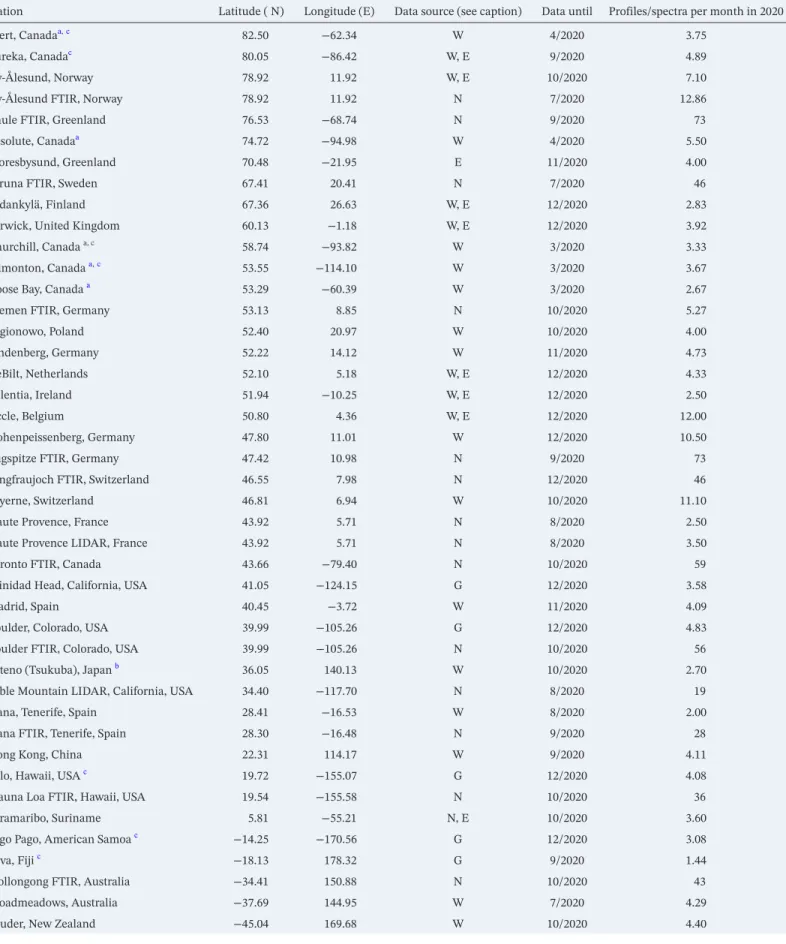
Ozonesondes measure profiles with high vertical resolution, about 100 m, and good accuracy, 5%–15% in the troposphere, 5% in the stratosphere (Smit et al., 2007; Sterling et al., 2018; Tarasick et al., 2016; Van Malderen et al., 2016; Witte et al., 2017; WMO, 2014). This is adequate to detect ozone anomalies of several percent. We use stations with regular soundings, at least once per month since the year 2000, and with data available until at least July 2020. Soundings with obvious deficiencies were rejected (i.e. large data gaps, integrated ozone column from the sounding deviating by more than 30% from ground- or satellite-based spectrometer measurement). Table 1 provides information on stations, and public data archives.
Apart from the sondes, FTIR spectrometers from the Network for the Detection of Atmospheric Compo-sition Change (NDACC, De Mazière et al., 2018) provide independent information, based on a completely different method (ground-based solar-infrared absorption spectrometry). The altitude resolution of FTIR ozone profiles in the troposphere is much coarser (5–10 km) than that of the sondes, while accuracy is simi-lar, 5%–10% (Vigouroux et al., 2015). Finally, we use data from tropospheric lidars (Gaudel et al., 2015; Gra-nados-Muñoz & Leblanc, 2016), which provide ozone profiles from ≈3 to 12 km altitude, with accuracy com-parable to the sondes (5%–10%; Leblanc et al., 2018), and slightly coarser altitude resolution (100 m–2 km). We also use global atmospheric composition re-analyses from the Copernicus Atmosphere Monitoring Ser-vice for the years 2003–2019, and operational analyses for the year 2020 (CAMS, Inness et al., 2019; see also Park et al., 2020). The CAMS data are taken at the grid-points closest to the stations in Table 1. The analy-ses (in 2020) are adjusted for the small average difference to the re-analyanaly-ses in 2018 and 2019. CAMS (re-) analyses are based on meteorological fields, and assimilation of satellite observations of ozone and NO2.
However, for NO2 the impact of the assimilation is small and frequently insignificant, so that tropospheric
NOx in CAMS is essentially controlled by the prescribed emissions (Inness et al., 2019). Similarly, the
lim-ited information content of current satellite measurements of tropospheric ozone means that tropospheric ozone in CAMS is also driven largely by the prescribed emissions (and the chemistry module). Stratospheric ozone, however, is constrained well by the assimilated satellite data. Thus, CAMS analyses account for the large Arctic stratospheric depletion in spring of 2020 (Manney et al., 2020; Wohltmann et al., 2020), for 2020 meteorological conditions, and for ozone transport, e.g. from the stratosphere to the troposphere (Neu et al., 2014). However, since they rely on “business as usual” emissions for 2020, the CAMS analyses do not account for the effects of COVID-19 emissions reductions in 2020 on tropospheric ozone (and NOx).
3. Results
For selected stations, Figure 1 presents the annual cycles of tropospheric ozone over the last 20 years, at 6 km, a representative altitude for the free troposphere. Monthly means (over 1 km wide layers) reduce syn-optic meteorological variability and measurement noise, and focus on longer-term, larger-scale variations. Payerne, Jungfraujoch, and Trinidad Head show an annual cycle with low ozone in winter and high ozone in summer. This is the case for most stations in the northern extratropics (Cooper et al., 2014; Gaudel et al., 2018; Parrish et al., 2020). Increased photochemical production due to more sunlight and warmer temperatures is the main driver for the summer ozone maximum in the northern extratropics (Archibald et al., 2020; Wu et al., 2007).
Figure 1 shows substantial yearly variability, but ozone levels are notably below average in 2020, at all four stations (thick red lines in Figure 1). At Payerne and Jungfraujoch, and a number of other stations, monthly means in spring and summer 2020 were actually the lowest, or close to the lowest, since 2000. For context, the dark blue lines in Figure 1 provide global CO2 emission reductions due to the COVD-19 pandemic (Le
Quéré et al., 2020b). Comparable reductions apply to global ozone precursor emissions (NOx and VOCs).
The (daily) emission reductions in Figure 1 indicate that the largest effect for ozone might be expected after March 2020. However, Figure 1 does not show any clear or close correspondence between unusual ozone monthly means in 2020 (red lines) and the emission reductions (dark blue lines).
Station Latitude ( N) Longitude (E) Data source (see caption) Data until Profiles/spectra per month in 2020
Alert, Canadaa,c 82.50 −62.34 W 4/2020 3.75
Eureka, Canadac 80.05 −86.42 W, E 9/2020 4.89
Ny-Ålesund, Norway 78.92 11.92 W, E 10/2020 7.10
Ny-Ålesund FTIR, Norway 78.92 11.92 N 7/2020 12.86
Thule FTIR, Greenland 76.53 −68.74 N 9/2020 73
Resolute, Canadaa 74.72 −94.98 W 4/2020 5.50
Scoresbysund, Greenland 70.48 −21.95 E 11/2020 4.00
Kiruna FTIR, Sweden 67.41 20.41 N 7/2020 46
Sodankylä, Finland 67.36 26.63 W, E 12/2020 2.83
Lerwick, United Kingdom 60.13 −1.18 W, E 12/2020 3.92
Churchill, Canada a, c 58.74 −93.82 W 3/2020 3.33
Edmonton, Canada a,c 53.55 −114.10 W 3/2020 3.67
Goose Bay, Canada a 53.29 −60.39 W 3/2020 2.67
Bremen FTIR, Germany 53.13 8.85 N 10/2020 5.27
Legionowo, Poland 52.40 20.97 W 10/2020 4.00 Lindenberg, Germany 52.22 14.12 W 11/2020 4.73 DeBilt, Netherlands 52.10 5.18 W, E 12/2020 4.33 Valentia, Ireland 51.94 −10.25 W, E 12/2020 2.50 Uccle, Belgium 50.80 4.36 W, E 12/2020 12.00 Hohenpeissenberg, Germany 47.80 11.01 W 12/2020 10.50
Zugspitze FTIR, Germany 47.42 10.98 N 9/2020 73
Jungfraujoch FTIR, Switzerland 46.55 7.98 N 12/2020 46
Payerne, Switzerland 46.81 6.94 W 10/2020 11.10
Haute Provence, France 43.92 5.71 N 8/2020 2.50
Haute Provence LIDAR, France 43.92 5.71 N 8/2020 3.50
Toronto FTIR, Canada 43.66 −79.40 N 10/2020 59
Trinidad Head, California, USA 41.05 −124.15 G 12/2020 3.58
Madrid, Spain 40.45 −3.72 W 11/2020 4.09
Boulder, Colorado, USA 39.99 −105.26 G 12/2020 4.83
Boulder FTIR, Colorado, USA 39.99 −105.26 N 10/2020 56
Tateno (Tsukuba), Japan b 36.05 140.13 W 10/2020 2.70
Table Mountain LIDAR, California, USA 34.40 −117.70 N 8/2020 19
Izana, Tenerife, Spain 28.41 −16.53 W 8/2020 2.00
Izana FTIR, Tenerife, Spain 28.30 −16.48 N 9/2020 28
Hong Kong, China 22.31 114.17 W 9/2020 4.11
Hilo, Hawaii, USA c 19.72 −155.07 G 12/2020 4.08
Mauna Loa FTIR, Hawaii, USA 19.54 −155.58 N 10/2020 36
Paramaribo, Suriname 5.81 −55.21 N, E 10/2020 3.60
Pago Pago, American Samoa c −14.25 −170.56 G 12/2020 3.08
Suva, Fiji c −18.13 178.32 G 9/2020 1.44
Wollongong FTIR, Australia −34.41 150.88 N 10/2020 43
Broadmeadows, Australia −37.69 144.95 W 7/2020 4.29
Lauder, New Zealand −45.04 169.68 W 10/2020 4.40
Table 1
Annual cycles of ozone anomalies, averaged over all northern extratropical stations (stations north of 15°N), are shown in Figure 2. Anomalies were defined as the relative deviation (in percent) from the 2000 to 2020 climatological mean of each calendar month at each station. As for the single stations in Figure 1, the ob-served northern extratropical average shows exceptionally low ozone throughout spring and summer 2020 (red line in Figure 2a). This is not reproduced by the CAMS analyses, which do not account for COVID-19 related emissions reductions, and simulate ozone in the usual range in 2020 (red line in Figure 2b). Again, there is no close temporal correspondence between the unusual behavior of observed ozone in 2020 (red line in Figure 2a), and the emission reductions (dark blue line in Figure 2a).
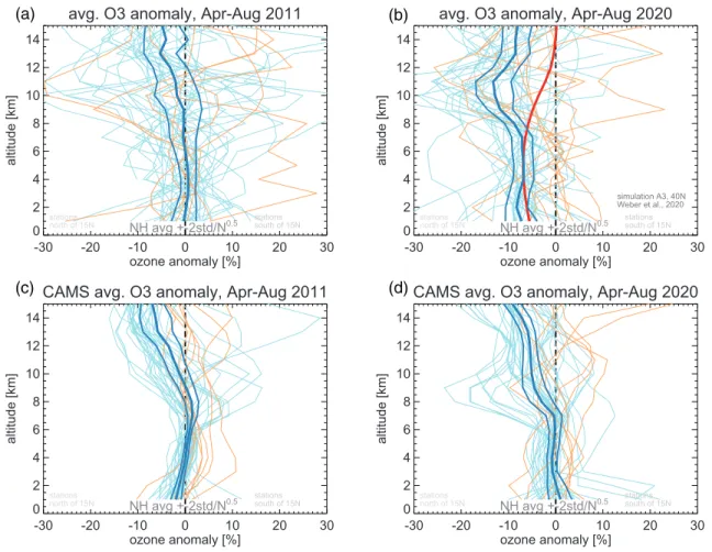
Figures 1 and 2 show large negative anomalies from April to August 2020. Figure 3 compares anomaly pro-files averaged over those five calendar months, between the years 2011 and 2020. Both years saw unusually large springtime ozone depletion in the Arctic stratosphere (Manney et al., 2020; Wohltmann et al., 2020). In the stratosphere, above ≈10 km, the Arctic depletion appears as low ozone, both in observations and CAMS results (particularly for stations north of 50°N). In both the stratosphere and the troposphere, the ob-served profiles show more variability than the smoother CAMS profiles. In 2020, most obob-served single sta-tion anomaly profiles (Figure 3b) are negative throughout the northern extratropical troposphere (between 1 and 10 km). This is not the case in 2011 (Figures 3a and 3c), nor in the CAMS data in 2020 (Figure 3d). The 2020 anomaly is even clearer for the northern extratropical mean profile (dark blue lines in Figure 3). The observed 2020 mean anomaly profile is large, −6% to −9%, and statistically significant at the 95% level (more than 99% in fact) from 1 to 8 km (Figure 3b), whereas the corresponding CAMS profile is close to zero (Figure 3d). Figure 3 indicates that Arctic stratospheric springtime ozone depletion did not have a large effect on tropospheric ozone below 8 km in 2011 and 2020 (see also model simulations in Figure S1, based on Gelaro et al., 2017, and Strahan et al., 2019), and that the CAMS “business as usual” simulation does not account for the observed large negative tropospheric anomaly in 2020.
Figure 3b also shows a simulated profile of tropospheric ozone reduction from a recent chemistry-climate modeling study of COVID-like emissions decreases by Weber et al. (2020). This simulated profile (red line in our Figure 3b) matches the observed northern extratropical ozone reduction (dark blue line), from the ground up to about 8 km. Above 8 km, the simulated profile deviates by ≈10% from the observed profile, because it assumes fixed 2012 to 2014 meteorological conditions. The CAMS analyses (Figure 3d) show that 2020 meteorological conditions and springtime Arctic stratospheric ozone depletion resulted in ozone reductions of 5%–10% above 9 km, consistent with the observations.
Time series of the tropospheric anomaly (averaged from April to August, and from 1 to 8 km altitude) are shown in Figure 4. In the observations (left panel), the year 2020 stands out with large negative anomalies, not seen in the CAMS data. Across the 20 previous years, ozone anomalies at individual stations (thin lines) are scattered around zero. The northern extratropical average anomaly (dark blue line) is usually smaller than ±3%. The only other observed exception is the positive anomaly related to the (European) heat-wave summer of 2003 (Vautard et al., 2007). The large negative northern extratropical anomaly in
Table 1
Continued
Station Latitude ( N) Longitude (E) Data source (see caption) Data until Profiles/spectra per month in 2020
Lauder FTIR, New Zealand −45.04 169.68 N 10/2020 99
Macquarie Island, Australia −54.50 158.94 W 7/2020 4.29
Data sources: W = World Ozone and UV Data Centre (https://woudc.org/archive/Archive-NewFormat/OzoneSonde_1.0_1/), N = Network for the Detection
of Atmospheric Composition Change (ftp://ftp.cpc.ncep.noaa.gov/ndacc/station/; ftp://ftp.cpc.ncep.noaa.gov/ndacc/RD/), E = European Space Agency
Validation Data Center (https://evdc.esa.int/ requires registration, or ftp://zardoz.nilu.no/nadir/projects/vintersol/data/o3sondes requires account),
G = Global Monitoring Laboratory, National Oceanic and Atmospheric Administration (ftp://aftp.cmdl.noaa.gov/data/ozwv/Ozonesonde/). FTIR, Fourier
Transform Infrared Spectrometers.
aDue to COVID-19 restrictions, most Canadian ozonesonde data were available only up to March or April 2020. bTateno data were corrected for the change
from Carbon Iodine to ECC ozonesondes in December 2009. cStations affected by a drop-off in ECC sonde sensitivity >3% in the stratosphere, after 2015 (see
Stauffer et al., 2020). The drop-off is much smaller (<<1%) in the troposphere, and should be negligible here. At many of the affected stations, ECC sondes behaved normally again in 2019/2020.
Figure 1. Observed ozone monthly means at four typical stations. Results are for 6 km altitude. The thick red line highlights the year 2020. Climatological
averages, and standard deviations over the years 2000–2020 are indicated by the thick black lines. Payerne (a) and Trinidad Head (c) are sonde stations. Jungfraujoch (b) is an FTIR station. Table Mountain (d) is a lidar station. Dark blue lines and scale on the right: CO2 emission reduction (in percent) from Le
Quéré et al. (2020b), as a proxy for ozone precursor reductions in 2020. FTIR, Fourier Transform Infrared Spectrometer.
Payerne, 6 km
JAN APR JUN AUG OCT DEC
month 0 20 40 60 80 100 ozone [nmol/mol] -20 0 reduction [% ]
CO2 emission reduction (Le Quere et al., 2020) 2000 to 2019 2020 avg +-1 std
Jungfraujoch FTIR, 6 km
JAN APR JUN AUG OCT DEC
month 0 20 40 60 80 100 ozone [nmol/mol] -20 0 reduction [% ]
CO2 emission reduction (Le Quere et al., 2020) 2000 to 2019 2020 avg +-1 std
Table Mountain Lidar, 6 km
JAN APR JUN AUG OCT DEC
month 0 20 40 60 80 100 ozone [nmol/mol] -20 0 reduction [% ]
CO2 emission reduction (Le Quere et al., 2020) 2000 to 2019 2020 avg +-1 std Trinidad_Head, 6 km
JAN APR JUN AUG OCT DEC
month 0 20 40 60 80 100 ozone [nmol/mol] -20 0 reduction [% ]
CO2 emission reduction (Le Quere et al., 2020) 2000 to 2019 2020 avg +-1 std
(a)
(c)
(d)
(b)
Figure 2. Annual cycles of monthly mean northern extratropical ozone anomalies at 6 km altitude. Anomalies are in
percent, relative to the climatological monthly mean calculated for each station/ instrument, and for the period 2000– 2020 (all Januaries, all Februaries, …, all Decembers). These single station/instrument anomalies are then averaged over all northern extratropical stations/instruments (north of 15°N). Panel (a) Results from the station observations. Panel (b) Results for CAMS atmospheric composition (re-)analyses at grid points nearest the stations. The CAMS data do not account for COVID-19 related emissions reductions in 2020. Gray lines: individual years from 2000 to 2019. Thick red line: year 2020. Thick black lines: average anomaly, ±1 standard deviation over the years. Dark blue lines and scale on the right in panel (a): Global CO2 emission reduction in 2020 (in percent) from Le Quéré et al. (2020b), as in Figure 1.
CAMS, Copernicus Atmosphere Monitoring Service.
NH average anomaly, 6 km
JAN APR JUN AUG OCT DEC
month -20 -15 -10 -5 0 5 10 15 ozone anomaly [% ] -20 0 reduction [% ]
CO2 emission reduction (Le Quere et al., 2020)
2000 to 2019 2020 avg +-1 std
CAMS NH average anomaly, 6 km
JAN APR JUN AUG OCT DEC
month -20 -15 -10 -5 0 5 10 15 ozone anomaly [% ] 2003 to 2019 2020 avg +-1 std
(a)
(b)
Figure 3. Ozone anomaly profiles (in percent), averaged over April to August. Stations are excluded in years where their data cover less than three of these five
months. Panel (a) for the year 2011. Panel (b) for the year 2020. Light blue lines: northern extratropical stations (north of 15°N). Light orange lines: remaining stations, south of 15°N. Thick dark blue line: mean of the northern extratropical stations. Thin dark blue lines: 95% confidence interval of the mean of the northern extratropical stations. Red line in panel (b): simulated ozone change at 40°N from Weber et al. (2020; Figure S4, scenario A3). Panels (c), (d): Same as (a), (b), but for CAMS (re-)analyses at the grid-points closest to the stations. CAMS, Copernicus Atmosphere Monitoring Service.
avg. O3 anomaly, Apr-Aug 2011
-30 -20 -10 0 10 20 30 ozone anomaly [%] 0 2 4 6 8 10 12 14 altitude [km] stations
north of 15N NH avg +-2std/N0.5 stationssouth of 15N
avg. O3 anomaly, Apr-Aug 2020
-30 -20 -10 0 10 20 30 ozone anomaly [%] 0 2 4 6 8 10 12 14 altitude [km] stations
north of 15N stationssouth of 15N
simulation A3, 40N Weber et al., 2020
NH avg +-2std/N0.5
CAMS avg. O3 anomaly, Apr-Aug 2020
-30 -20 -10 0 10 20 30 ozone anomaly [%] 0 2 4 6 8 10 12 14 altitude [km] stations
north of 15N NH avg +-2std/N0.5 stationssouth of 15N
CAMS avg. O3 anomaly, Apr-Aug 2011
-30 -20 -10 0 10 20 30 ozone anomaly [%] 0 2 4 6 8 10 12 14 altitude [km] stations
north of 15N NH avg +-2std/N0.5 stationssouth of 15N
(b)
(d)
(c)
(a)
Figure 4. Tropospheric ozone anomaly, averaged over April to August and from 1 to 8 km, for the years 2000–2020.
Panel (a) Observations. Panel (b) CAMS atmospheric composition (re-)analyses. Light blue lines: northern extratropical stations (north of 15°N). Light orange lines: stations south of 15°N. Thick dark blue line: Average over all stations north of 15°N. Thin dark blue lines: ±2 standard deviations over all years of this average. CAMS, Copernicus Atmosphere Monitoring Service.
avg. O3 anomaly, 1-8km, Apr-Aug
2000 2005 2010 2015 2020 -20 -10 0 10 20 average anomaly [% ] stations north of 15N stations south of 15N NH avg, 0+-2std
CAMS avg. O3 anomaly, 1-8km, Apr-Aug
2000 2005 2010 2015 2020 -20 -10 0 10 20 average anomaly [% ] stations north of 15N stations south of 15N NH avg, 0+-2std
(a)
(b)
the observations in 2020, ≈−7%, is clearly outside of the ±2σ range of the previous 20 years (thin dark blue lines). It is not reproduced by the CAMS “emissions as usual” analysis.
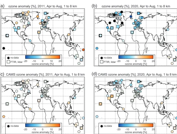
The geographic distribution of the average tropospheric ozone anomalies is shown for 2011 and 2020 in Fig-ure 5. 2020 stands out in the observations with large negative anomalies at nearly all northern extratropical stations, and a fairly uniform geographical distribution (see Table S1 of the supplement for the numerical values). CAMS does show negative anomalies in 2020, but only north of 50°N, and not as large as the ob-servations. In the Southern Hemisphere in 2020, agreement between observations and CAMS is quite good, typically within 2.5% or better (see also Table S1). In 2011, some stations show positive anomalies, negative anomalies are not as large as in 2020, and the geographical distribution is less uniform. Agreement between observations and CAMS is reasonable in 2011, usually within a few percent.
4. Discussion and Conclusions
Ozone stations in the northern extratropics indicate exceptionally low ozone in the free troposphere (1–8 km) in spring and summer 2020. Compared to the 2000–2020 climatology, ozone was reduced by 7% (≈4 nmol/mol). Such widespread low tropospheric ozone, across so many stations and over several months has not been observed in any previous year since 2000. The observed 7% ozone reduction in the free tropo-sphere stands in contrast to increases of surface ozone by 10%–30%, reported for many polluted urban areas after the COVID-19 related emissions reductions in 2020 (e.g., Collivignarelli et al., 2020; Lee et al., 2020; Shi & Brasseur, 2020; Siciliano et al., 2020; Venter et al., 2020). However, the chemical regime for ozone in the free troposphere is different (e.g., Kroll et al., 2020; Sillman, 1999; Thornton et al., 2002), and free tropospheric ozone reductions are expected after the substantial decrease of precursor emissions due to the COVID-19 pandemic (e.g. Guevara et al., 2020; Zhang et al., 2020).
Figure 5. Geographic distribution of observed tropospheric ozone anomalies (averaged over the months April to
August, and over altitudes from 1 to 8 km) for the years (a) 2011 and (b) 2020. Panels (c) and (d): same, but for CAMS results at the station locations. Colored circles give the anomaly at the ozonesonde stations. Squares are for FTIR and lidar stations. See Table S1 of the supplement for the numerical values. Black filling indicates insufficient data in the given year. CAMS, Copernicus Atmosphere Monitoring Service; FTIR, Fourier Transform Infrared Spectrometers.
ozone anomaly [%], 2011, Apr to Aug, 1 to 8 km
FTIR, lidar nodata
-20 -10 0 10 20
ozone anomaly [%]
ozone anomaly [%], 2020, Apr to Aug, 1 to 8 km
FTIR, lidar nodata
-20 -10 0 10 20
ozone anomaly [%]
CAMS ozone anomaly [%], 2020, Apr to Aug, 1 to 8 km
nodata
-20 -10 0 10 20
ozone anomaly [%] CAMS ozone anomaly [%], 2011, Apr to Aug, 1 to 8 km
nodata -20 -10 0 10 20 ozone anomaly [%]
(c)
(a)
(d)
(b)
Recent model simulations of COVID-like emissions decreases (Weber et al., 2020) find tropospheric ozone reductions very similar to our observational results. From our results, and the simulations by Weber et al., 2020, it appears that the total tropospheric ozone burden of the northern extratropics decreased by about 7% for April–August 2020. The contribution from ozone increases in polluted urban areas to the total burden is opposite, but very small.
The Weber et al. (2020) simulations indicate that the major causes of tropospheric ozone reduction come from reduced surface transportation (ozone decrease throughout most of the northern extratropical trop-osphere), and from reduced aviation (ozone decrease mostly between 10 and 12 km altitude and north of 30°N, see also Grewe et al., 2017). While the simulations are qualitatively consistent with the observations, they consider only March to May. New simulations using more recent and extended emissions estimates (Le Quéré et al., 2020b), and further comparison with our station observations would be worthwhile.
The observed large and fairly uniform 7% reduction of ozone in the northern extratropical troposphere in spring and summer 2020 provides a far reaching test case for the response of tropospheric ozone to emis-sion changes. Further quantification of this anomaly will be possible, when observations from commercial aircraft (IAGOS), and satellite instruments become available. Additional modeling studies will improve our understanding of the contributions from different sectors such as air traffic, and surface transportation.
Data Availability Statement
Most of the ozonesonde data used in this study are freely available from the World Ozone and UV Data Center (https://woudc.org) at Environment Canada (https://exp-studies.tor.ec.gc.ca/), and are downloada-ble at https://woudc.org/archive/Archive-NewFormat/OzoneSonde_1.0_1/).
Some ozonesonde data for 2020 were not yet available at the WOUDC. Instead, rapid delivery data were obtained from ftp://zardoz.nilu.no/nadir/projects/vintersol/data/o3sondes (requires registration), at the Nadir database of the Norwegian Institute for Air Quality (NILU, https://projects.nilu.no/nadir/obs.html). Registration information, and the same data in a different format, are available from the European Space Agency Validation Data Center (https://evdc.esa.int/).
For Boulder, Trinidad Head, Hilo, Fiji, and Samoa, stations operated by the US National Oceanic and Atmospheric Administration, Global Monitoring Laboratory (https://www.esrl.noaa.gov/gmd/ozwv/), data can be obtained freely from ftp://aftp.cmdl.noaa.gov/data/ozwv/Ozonesonde/.
FTIR and lidar data, as well as some ozonesonde data, are from the Network for the Detection of At-mospheric Composition Change (https://ndacc.org), and are freely available at ftp://ftp.cpc.ncep.noaa.gov/
ndacc/station/ and ftp://ftp.cpc.ncep.noaa.gov/ndacc/RD/.
Copernicus Atmosphere Monitoring Service (CAMS) global chemical weather EAC4 re-analyses are available at https://atmosphere.copernicus.eu/data. CAMS operational global analyses and forecasts are available at https://apps.ecmwf.int/datasets/data/cams-nrealtime/.
References
Archibald, A. T., Neu, J. L., Elshorbany, Y., Cooper, O. R., Young, P. J., Akiyoshi, H., et al. (2020). Tropospheric Ozone Assessment Report: A critical review of changes in the tropospheric ozone burden and budget from 1850 to 2100. Elementa Science of the Anthropocene, 8, 034. https://doi.org/10.1525/elementa.2020.034
Barré, J., Petetin, H., Colette, A., Guevara, M., Peuch, V. -H., Rouil, L., et al. (2020). Estimating lockdown induced European NO2 changes.
Atmospheric Chemistry and Physics Discussions. 1–28. https://doi.org/10.5194/acp-2020-995
Bauwens, M., Compernolle, S., Stavrakou, T., Müller, J.-F., van Gent, J., Eskes, H., et al. (2020). Impact of coronavirus outbreak on NO2 pollution assessed using TROPOMI and OMI observations. Geophysical Research Letters, 47, e2020GL087978. https://doi.
org/10.1029/2020GL087978
Bozem, H., Butler, T. M., Lawrence, M. G., Harder, H., Martinez, M., Kubistin, D., et al. (2017). Chemical processes related to net ozone tendencies in the free troposphere. Atmospheric Chemistry and Physics, 17, 10565–10582. https://doi.org/10.5194/acp-17-10565-2017 Chen, L.-W. A., Chien, L.-C., Li, Y., & Lin, G. (2020). Nonuniform impacts of COVID-19 lockdown on air quality over the United States.
The Science of the Total Environment, 745, 141105. https://doi.org/10.1016/j.scitotenv.2020.141105
Collivignarelli, M. C., Abbà, A., Bertanza, G., Pedrazzani, R., Ricciardi, P., & Carnevale Miino, M. (2020). Lockdown for COVID-2019 in Mi-lan: What are the effects on air quality? The Science of the Total Environment, 732, 139280. https://doi.org/10.1016/j.scitotenv.2020.139280 Cooper, O. R., Parrish, D. D., Ziemke, J., Balashov, N. V., Cupeiro, M., Galbally, I. E., et al. (2014). Global distribution and trends of tropospheric ozone: An observation-based review. Elementa: Science of the Anthropocene, 2, 000029. https://doi.org/10.12952/journal.elementa.000029 Acknowledgments
The authors greatly acknowledge the know-how and the hard work of station personnel launching the ozonesondes and taking the ground-based meas-urements. Without their dedicated efforts over many years, and especially during the COVID-19 lockdowns in 2020, investigations like this one are not possible!
Deutscher Wetterdienst funds the ozone program at Hohenpeißenberg and makes research like this possible. NOAA GML supported additional launches in Boulder and Trinidad Head in April and May 2020. NOAA and NA-SA's Upper Atmosphere Composition Observations (UACO) Program support
De Mazière, M., Thompson, A. M., Kurylo, M. J., Wild, J. D., Bernhard, G., Blumenstock, T., et al. (2018). The Network for the Detection of Atmospheric Composition Change (NDACC): History, status and perspectives. Atmospheric Chemistry and Physics, 18, 4935–4964. https://doi.org/10.5194/acp-18-4935-2018
Dentener, F., Keating, T. T., & Akimoto, H. (Eds.), (2011). Hemispheric transport of air pollution 2010, Part A: Ozone and particulate matter. Air pollution studies (Vol. 17, p. 305). New York: United Nations. https://doi.org/10.18356/2c908168-en
Ding, J., van der A, R. J., Eskes, H. J., Mijling, B., Stavrakou, T., van Geffen, J. H., et al. (2020). NOx emissions reduction and rebound in
China due to the COVID-19 crisis. Geophysical Research Letters, 46, e2020GL089912. https://doi.org/10.1029/2020GL089912 Feng, S., Jiang, F., Wang, H., Wang, H., Ju, W., Shen, Y., et al. (2020). NOx emission changes over China during the COVID-19 epidemic
inferred from surface NO2 observations. Geophysical Research Letters, 47, e2020GL090080. https://doi.org/10.1029/2020GL090080
Gaudel, A., Ancellet, G., & Godin-Beekmann, S. (2015). Analysis of 20 years of tropospheric ozone vertical profiles by lidar and ECC at Obser-vatoire de Haute Provence (OHP) at 44°N, 6.7°E. Atmospheric Environment, 113, 78–89. https://doi.org/10.1016/j.atmosenv.2015.04.028 Gaudel, A., Cooper, O. R., Ancellet, G., Barret, B., Boynard, A., Burrows, J. P., et al. (2018). Tropospheric Ozone Assessment Report: Pres-ent-day distribution and trends of tropospheric ozone relevant to climate and global atmospheric chemistry model evaluation. Elementa
Science of the Anthropocene, 6, 39. https://doi.org/10.1525/elementa.291
Gelaro, R., McCarty, W., Suarez, M. J., Todling, R., Molod, A., Takacs, et al. (2017). The Modern-Era Retrospective Analysis for Research and Applications, version 2 (MERRA-2). Journal of Climate, 30, 5419–5454. https://doi.org/10.1175/JCLI-D-16-0758.1
Goldberg, D. L., Anenberg, S. C., Griffin, D., McLinden, C. A., Lu, Z., & Streets, D. G. (2020). Disentangling the impact of the COVID-19 lock-downs on urban NO2 from natural variability. Geophysical Research Letters, 47, e2020GL089269. https://doi.org/10.1029/2020GL089269
Granados-Muñoz, M. J., & Leblanc, T. (2016). Tropospheric ozone seasonal and long-term variability as seen by lidar and surface meas-urements at the JPL-Table Mountain Facility, California. Atmospheric Chemistry and Physics, 16, 9299–9319. https://doi.org/10.5194/ acp-16-9299-2016
Grewe, V., Dahlmann, K., Flink, J., Frömming, C., Ghosh, R., Gierens, et al. (2017). Mitigating the climate impact from aviation: Achieve-ments and results of the DLR WeCare project. Aerospace, 4, 34. https://doi.org/10.3390/aerospace4030034
Guevara, M., Jorba, O., Soret, A., Petetin, H., Bowdalo, D., Serradell, K., et al. (2020). Time-resolved emission reductions for atmospher-ic chemistry modelling in Europe during the COVID-19 lockdowns. Atmospheratmospher-ic Chemistry and Physatmospher-ics, 21, 773–797. https://doi. org/10.5194/acp-2020-686
Hurtmans, D., Coheur, P.-F., Wespes, C., Clarisse, L., Scharf, O., Clerbaux, C., et al. (2012). FORLI radiative transfer and retrieval code for IASI. Journal of Quantitative Spectroscopy and Radiative Transfer, 113, 1391–1408. https://doi.org/10.1016/j.jqsrt.2012.02.036 Inness, A., Ades, M., Agusti-Panareda, A., Barré, J., Benedictow, A., Blechschmidt, A. M., et al. (2019). The CAMS reanalysis of
atmospher-ic composition. Atmospheratmospher-ic Chemistry and Physatmospher-ics, 19, 3515–3556. https://doi.org/10.5194/acp-19-3515-2019
Keller, C. A., Evans, M. J., Knowland, K. E., Hasenkopf, C. A., Modekurty, S., Lucchesi, R. A., et al. (2021). Global impact of COVID-19 restrictions on the surface Concentrations of nitrogen dioxide and ozone. Atmospheric Chemistry and Physics Discussions, 1–32. https:// doi.org/10.5194/acp-2020-685
Kroll, J. H., Heald, C. L., Cappa, C. D., Farmer, D. K., Fry, J. L., Murphy, J. G., & Steiner, A. L. (2020). The complex chemical effects of COVID-19 shutdowns on air quality. Nature Chemistry, 12, 777–779. https://doi.org/10.1038/s41557-020-0535-z
Le Quéré, C., Jackson, R. B., Jones, M. W., Smith, A. J. P., Abernethy, S., Andrew, R. M., et al. (2020a). Temporary reduction in dai-ly global CO2 emissions during the COVID-19 forced confinement. Nature Climate Change, 10, 647–653. https://doi.org/10.1038/
s41558-020-0797-x
Le Quéré, C., Jackson, R. B., Jones, M. W., Smith, A. J. P., Abernethy, S., Andrew, R. M., et al. (2020b). Supplementary data to: Le Quéré et al (2020), Temporary reduction in daily global CO2 emissions during the COVID-19 forced confinement (Version 1.2). Global Carbon
Project, 10, 647–653. https://doi.org/10.18160/RQDW-BTJU
Leblanc, T., Brewer, M. A., Wang, P. S., Granados-Muñoz, M. J., Strawbridge, K. B., Travis, M., et al. (2018). Validation of the TOLNet lidars: the Southern California Ozone Observation Project (SCOOP). Atmospheric Measurement Techniques, 11, 6137–6162. https://doi. org/10.5194/amt-11-6137-2018
Lee, J. D., Drysdale, W. S., Finch, D. P., Wilde, S. E., & Palmer, P. I. (2020). UK surface NO2 levels dropped by 42 % during the COVID-19
lockdown: impact on surface O3. Atmospheric Chemistry and Physics, 20, 15743–15759. https://doi.org/10.5194/acp-20-15743-2020 Liu, X., Bhartia, P. K., Chance, K., Spurr, R. J. D., & Kurosu, T. P. (2010). Ozone profile retrievals from the ozone monitoring instrument.
Atmospheric Chemistry and Physics, 10, 2521–2537. https://doi.org/10.5194/acp-10-2521-2010
Liu, Z., Ciais, P., Deng, Z., Lei, R., Davis, S. J., Feng, S., et al. (2020). Near-real-time monitoring of global CO2 emissions reveals the effects
of the COVID-19 pandemic. Nature Communications, 11, 5172. https://doi.org/10.1038/s41467-020-18922-7
Manney, G. L., Livesey, N. J., Santee, M. L., Froidevaux, L., Lambert, A., Lawrence, Z. D., et al. (2020). Record-low Arctic stratospheric ozone in 2020: MLS observations of chemical processes and comparisons with previous extreme winters. Geophysical Research Letters,
47, e2020GL089063. https://doi.org/10.1029/2020GL089063
Menut, L., Bessagnet, B., Siour, G., Mailler, S., Pennel, R., & Cholakian, A. (2020). Impact of lockdown measures to combat COVID-19 on air quality over western Europe. The Science of the Total Environment, 741, 140426. https://doi.org/10.1016/j.scitotenv.2020.140426 Nédélec, P., Blot, R., Boulanger, D., Athier, G., Cousin, J.-M., Gautron, B., et al. (2015). Instrumentation on commercial aircraft for
moni-toring the atmospheric composition on a global scale: The IAGOS system, technical overview of ozone and carbon monoxide measure-ments. Tellus B: Chemical and Physical Meteorology, 67, 27791. https://doi.org/10.3402/tellusb.v67.27791
Neu, J., Flury, T., Manney, G., Santee, M. L., Livesey, N. J., & Worden, J. (2014). Tropospheric ozone variations governed by changes in stratospheric circulation. Nature Geoscience, 7, 340–344. https://doi.org/10.1038/ngeo2138
Oetjen, H., Payne, V. H., Kulawik, S. S., Eldering, A., Worden, J., Edwards, D. P., et al. (2014). Extending the satellite data record of trop-ospheric ozone profiles from Aura-TES to MetOp-IASI: Characterisation of optimal estimation retrievals. Atmtrop-ospheric Measurement
Techniques, 7, 4223–4236. https://doi.org/10.5194/amt-7-4223-2014
Ordóñez, C., Garrido-Perez, J. M., & García-Herrera, R. (2020). Early spring near-surface ozone in Europe during the COVID-19 shut-down: Meteorological effects outweigh emission changes. The Science of the Total Environment, 747, 141322. https://doi.org/10.1016/j. scitotenv.2020.141322
Park, S., Son, S.-W., Jung, M.-I., Park, J., & Park, S.-S. (2020). Evaluation of tropospheric ozone reanalyses with independent ozonesonde observations in East Asia. Geoscience Letters, 7, 12. https://doi.org/10.1186/s40562-020-00161-9
Parrish, D. D., Derwent, R. G., Steinbrecht, W., Stübi, R., Van Malderen, R., Steinbacher, M., et al. (2020). Zonal similarity of long-term changes and seasonal cycles of baseline ozone at northern midlatitudes. Journal of Geophysical Research: Atmosphere, 125, e2019JD031908. https://doi.org/10.1029/2019JD031908
the SHADOZ ozone soundings at Hilo, Pago-Pago (American Samoa) and Suva (Fiji). UACO also provides partial support for the Boulder FTIR and the Table Mountain Lidar.
The NDACC FTIR stations Bremen, Ny-Ålesund, Izaña, Kiruna, and Zugspitze have been supported by the German Bundesministerium für Wirtschaft und Energie (BMWi) via DLR under grants 50EE1711A, 50EE1711B, and 50EE1711D. Izaña, Kiruna, and Zugspitze have also been supported by the Helmholtz Society via the research program ATMO.
The FTIR measurements in Bremen and Ny-Ålesund receive additional support by the Senate of Bremen, the FTIR measurements in Ny-Ålesund also by AWI Bremerhaven. The University of Bremen further acknowledges funding by DFG (German research foundation) TRR 172, Project Number 268020496, within the Transregional Collaborative Research Center “ArctiC Amplifica-tion: Climate Relevant Atmospheric and SurfaCe Processes, and Feedback Mechanisms (AC)3.”
The University of Liège contribution has been supported primarily by the Fonds de la Recherche Scientifique, FNRS under grant J.0147.18, as well as by the CAMS project. EM is a senior research associate of the F.R.S.-FNRS. The Toronto FTIR measurements were supported by Environment and Climate Change Canada, the Natural Sciences and Engineering Research Council of Canada (NSERC), and the NSERC CRE-ATE Training Program in Technologies for Exo-Planetary Science.
The University of the Wollongong thanks the Australian Research Council that has provided significant support over the years for the NDACC site at Wollongong, most recently as part of project DP160101598.
Part of this research work was carried out at the Jet Propulsion Laboratory, California Institute of Technology, under a contract with the National Aeronautics and Space Administration (80NM0018D004).
The National Center for Atmospheric Research is sponsored by the National Science Foundation. The NCAR FTS observation programs at Thule, GR and Boulder, CO are supported under contract by the National Aeronautics and Space Administration (NASA). The Thule work is also supported by the NSF Office of Polar Programs (OPP). We wish to thank the Danish Meteorological Institute for support at the Thule site and NOAA for support of the MLO site.
Key results for this manuscript were generated using Copernicus Atmos-phere Monitoring Service Information from the European Community. No author reports a financial (or other) conflict of interest.
Shi, X., & Brasseur, G. P. (2020). The response in air quality to the reduction of Chinese economic activities during the COVID-19 outbreak.
Geophysical Research Letters, 47, e2020GL088070. https://doi.org/10.1029/2020GL088070
Sicard, P., De Marco, A., Agathokleous, E., Feng, Z., Xu, X., Paoletti, E., et al. (2020). Amplified ozone pollution in cities during the COV-ID-19 lockdown. The Science of the Total Environment, 735, 139542. https://doi.org/10.1016/j.scitotenv.2020.139542
Siciliano, B., Dantas, G., da Silva, C. M., & Arbilla, G. (2020). Increased ozone levels during the COVID-19 lockdown: Analysis for the city of Rio de Janeiro, Brazil. The Science of the Total Environment, 737, 139765. https://doi.org/10.1016/j.scitotenv.2020.139765
Sillman, S. (1999). The relation between ozone, NOx and hydrocarbons in urban and polluted rural environments. Atmospheric
Environ-ment, 33, 1821–1845. https://doi.org/10.1016/S1352-2310(98)00345-8
Smit, H. G. J., Straeter, W., Johnson, B., Oltmans, S., Davies, J., Tarasick, D. W., et al. (2007). Assessment of the performance of ECC-ozone-sondes under quasi-flight conditions in the environmental simulation chamber: Insights from the Jülich Ozone Sonde Intercomparison Experiment (JOSIE). Journal of Geophysical Research, 112, D19306. https://doi.org/10.1029/2006JD007308
Stauffer, R. M., Thompson, A. M., Kollonige, D. E., Witte, J. C., Tarasick, D. W., Davies, J., et al. (2020). A post-2013 dropoff in total ozone at a third of global ozonesonde stations: Electrochemical concentration cell instrument artifacts? Geophysical Research Letters, 47, e2019GL086791. https://doi.org/10.1029/2019GL086791
Sterling, C. W., Johnson, D. J., Oltmans, S. J., Smit, H. G. J., Jordan, A. F., Cullis, P. D., et al. (2018). Homogenizing and estimating the uncertainty in NOAA's long-term vertical ozone profile records measured with the electrochemical concentration cell ozonesonde.
Atmospheric Measurement Techniques, 11, 3661–3687. https://doi.org/10.5194/amt-11-3661-2018
Strahan, S. E., Douglass, A. R., & Damon, M. R. (2019). Why do Antarctic ozone recovery trends vary? Journal of Geophysical Research:
Atmosphere, 124, 8837–8850. https://doi.org/10.1029/2019JD030996
Tarasick, D. W., Davies, J., Smit, H. G. J., & Oltmans, S. J. (2016). A re-evaluated Canadian ozonesonde record: measurements of the ver-tical distribution of ozone over Canada from 1966 to 2013. Atmospheric Measurement Techniques, 9, 195–214. https://doi.org/10.5194/ amt-9-195-2016
Tarasick, D., Galbally, I. E., Cooper, O. R., Schultz, M. G., Ancellet, G., Leblanc, T., et al. (2019). Tropospheric Ozone Assessment Report: Tropospheric ozone from 1877 to 2016, observed levels, trends and uncertainties. Elementa Science of the Anthropocene, 7, 39. https:// doi.org/10.1525/elementa.376
Thornton, J. A., Wooldridge, P. J., Cohen, R. C., Martinez, M., Harder, H., Brune, W. H., et al. (2002). Ozone production rates as a func-tion of NOx abundances and HOx production rates in Nashville urban plume. Journal of Geophysical Research, 107, 4146. https://doi.
org/10.1029/2001JD000932
Van Malderen, R., Allaart, M. A. F., De Backer, H., Smit, H. G. J., & De Muer, D. (2016). On instrumental errors and related correction strategies of ozonesondes: Possible effect on calculated ozone trends for the nearby sites Uccle and De Bilt. Atmospheric Measurement
Techniques, 9, 3793–3816. https://doi.org/10.5194/amt-9-3793-2016
Vautard, R., Beekmann, M., Desplat, J., Hodzic, A., & Morel, S. (2007). Air quality in Europe during the summer of 2003 as a prototype of air quality in a warmer climate. Comptes Rendus Geoscience, 339, 747–763. https://doi.org/10.1016/j.crte.2007.08.003
Venter, Z. S., Aunan, K., Chowdhury, S., & Lelieveld, J. (2020). COVID-19 lockdowns cause global air pollution declines. Proceedings of the
National Academy of Sciences, 117(32), 18984–18990. https://doi.org/10.1073/pnas.2006853117
Vigouroux, C., Blumenstock, T., Coffey, M., Errera, Q., García, O., Jones, N. B., et al. (2015). Trends of ozone total columns and vertical distribution from FTIR observations at eight NDACC stations around the globe. Atmospheric Chemistry and Physics, 15, 2915–2933. https://doi.org/10.5194/acp-15-2915-2015
Weber, J., Shin, Y. M., Staunton Sykes, J., Archer-Nicholls, S., Abraham, N. L., & Archibald, A. T. (2020). Minimal climate impacts from short-lived climate forcers following emission reductions related to the COVID-19 pandemic. Geophysical Research Letters, 47, e2020GL090326. https://doi.org/10.1029/2020GL090326
Witte, J. C., Thompson, A. M., Smit, H. G. J., Fujiwara, M., Posny, F., Coetzee, G. J. R., et al. (2017). First reprocessing of Southern Hem-isphere ADditional OZonesondes (SHADOZ) profile records (1998–2015): 1. Methodology and evaluation. Journal of Geophysical
Re-search: Atmosphere, 122, 6611–6636. https://doi.org/10.1002/2016JD026403
WMOASOPOS panel. (2014). Quality assurance and quality control for ozonesonde measurements in GAW, World Meteorological Organi-zation (WMO), Global Atmosphere Watch report series. H. G. J. Smit (Ed.), GAW Report No. 201 (p. 100). Geneva. Retrieved from https:// library.wmo.int/doc_num.php?explnum_id=7167
Wohltmann, I., von der Gathen, P., Lehmann, R., Maturilli, M., Deckelmann, H., Manney, G. L., et al. (2020). Near-complete local reduc-tion of Arctic stratospheric ozone by severe chemical loss in spring 2020. Geophysical Research Letters, 47, e2020GL089547. https://doi. org/10.1029/2020GL089547
Wu, S., Mickley, L. J., Jacob, D. J., Logan, J. A., Yantosca, R. M., & Rind, D. (2007). Why are there large differences between models in global budgets of tropospheric ozone? Journal of Geophysical Research, 112, D05302. https://doi.org/10.1029/2006JD007801
Zhang, Y., West, J. J., Emmons, L. K., Flemming, J., Jonson, J. E., Lund, M. T., et al. (2020). Contributions of world regions to the global tropospheric ozone burden change from 1980 to 2010. Geophysical Research Letters, 47, e2020GL089184. https://doi. org/10.1029/2020GL089184