HAL Id: tel-03215903
https://tel.archives-ouvertes.fr/tel-03215903
Submitted on 3 May 2021
HAL is a multi-disciplinary open access archive for the deposit and dissemination of sci-entific research documents, whether they are pub-lished or not. The documents may come from teaching and research institutions in France or abroad, or from public or private research centers.
L’archive ouverte pluridisciplinaire HAL, est destinée au dépôt et à la diffusion de documents scientifiques de niveau recherche, publiés ou non, émanant des établissements d’enseignement et de recherche français ou étrangers, des laboratoires publics ou privés.
its variations with sea surface temperature using a
constellation of satellites
Erik Höjgård-Olsen
To cite this version:
Erik Höjgård-Olsen. Observations of the tropical atmospheric water cycle and its variations with sea surface temperature using a constellation of satellites. Ocean, Atmosphere. Université Paris-Saclay, 2020. English. �NNT : 2020UPASJ007�. �tel-03215903�
Observations du cycle de l’eau atmosphérique
tropicale et de ses variations avec la
température de surface de la mer,
à l’aide d’une constellation de satellites
Observations of the Tropical Atmospheric Water Cycle,
Using a Constellation of Satellites
Thèse de doctorat de l'université Paris-Saclay
École doctorale n°129, sciences de l’environnement d’Île-de-France (SEIF) Spécialité de doctorat: Océan, atmosphère, climat et observations spatiales
Unité de recherche : Université Paris-Saclay, UVSQ, CNRS, LATMOS, 78280, Guyancourt, France. Référent : Université de Versailles Saint-Quentin-en-Yvelines
Thèse présentée et soutenue à Paris-Saclay,
le 27/11/2020, par
Erik HÖJGÅRD-OLSEN
Composition du Jury
Philippe BOUSQUET
Professeur des universités, UVSQ/LSCE Président
Jean-Pierre CHABOUREAU
Physicien, HDR, UPS/LA Rapporteur & Examinateur
Céline CORNET
Professeure, UDL/LOA Rapporteure & Examinatrice
Dominique BOUNIOL
Chargée de Recherche, UPS/CNRS Examinatrice
Direction de la thèse
Hélène BROGNIEZ
Maitresse de Conférence, UVSQ/LATMOS Directrice de thèse
Hélène CHEPFER
Professeure, UPMC/LMD Co-directrice de thèse
Laurence PICON
Professeure, UPMC/LMD Invitée
Th
èse
de
do
ct
or
at
NNT : 202 0U PA SJ 00 7Maison du doctorat de l’Université Paris-Saclay
2ème étage aile ouest, Ecole normale supérieure Paris-Saclay
4 avenue des Sciences, 91190 Gif sur Yvette, France
Acknowledgements
First, I would like to direct a most sincere thank you to my thesis supervisors, Hélène Brogniez and Hélène Chepfer, for three years of pedagogic guidance and dedication to my work.
I would also like to thank the directors of my hosting laboratories Philippe Keckhut and François Ravetta (LATMOS) and Philippe Drobinski (LMD), as well as the administrative offices for managing the labs – especially during the exceptional circumstances of 2020.
I want to thank all the members of the jury for accepting to examine my thesis. Thanks to Philippe Bousquet for having accepted to chair the jury, and thank you Jean-Pierre Chaboureau and Céline Cornet for agreeing to be the reporters of my manuscript.
Thank you to Dominique Bouniol and Tristan L’Ecuyer for following my progress as members of my thesis committee and for fruitful discussions during our meetings.
At LATMOS and LMD, I want to thank the SPACE team and Cloud teams. I want to especially thank the people whose help made my thesis possible: Hélène Brogniez, Hélène Chepfer, Christophe Dufour, Rodrigo Guzman, Patrick Raberanto, and Artem Feofilov.
I want to direct a special thanks to Rodrigo Guzman for the time he took to help me get settled with the software and administrative issues during the first months of my PhD.
I want to thank the social groups at LMD and LATMOS for many pleasant and relaxed social engagements. I especially want to thank Melissa, Oscar, Pragya and Minh with whom I have shared countless enjoyable moments and hilarious conversations. Thank you also to Eivind, Léo, Bastien, Nicolas, Artemis, Aurelie, Fuxing, Felipe, Antonin, Olivier, Assia, Navi, Thibault, Alexis, Stavros, Fausto, Sakina, Cyprien, Chloé...
A final and most sincere thank you to my family and friends back in Scandinavia, for their love, support and encouragements during my adventure.
Table of Content
Introduction ...1
1 Context ...6
1.1 Complexity Facets of the Atmospheric Water Cycle ...7
1.2 Radiation and the Water Cycle ... 12
1.3 Principal Hypotheses About the Tropical Atmospheric Water Cycle’s Response to Surface Warming ... 19
1.4 Present Day Limitations with Observations and Models ... 23
1.5 Principal Science Questions ... 26
2 The Synergistic Dataset ... 29
2.1 Introduction to the Dataset ... 30
2.2 Relative Humidity from SAPHIR ... 32
2.3 Cloud Characteristics from GOCCP ... 40
2.4 Near-Surface Precipitation from the CloudSat 2C-PRECIP-COLUMN Product ... 47
2.5 Surface Temperature and Vertical Pressure Velocity from ERA5 ... 54
2.6 Satellite Collocations ... 57
3 Variations on the Instantaneous Timescale Under Large-Scale Circulation Constraints ... 62
Summary of the Paper and Its Main Outcomes ... 63
3.1 Introduction ... 69
3.2 Data ... 70
3.3 Methods ... 72
3.4 Analyses of the Tropical Atmospheric Water Cycle’s Variation with SST in Different Regimes ... 78
3.5 Discussion ... 87
3.6 Conclusion ... 91
4 Covariations on Different Temporal and Spatial Scales... 94
4.1 Introduction ... 95
4.2 Method ... 98
4.3 Analysis of Observed Water Cycle Variable Covariations on Different Timescales ... 104
4.4 Discussion of These Results... 119
4.5 Summary and Conclusions... 125
Appendices ... 135
A Basic Radiative Transfer Equations ... 136
B Supporting Data Information ... 138
C Supplementary Figures of Höjgård-Olsen et al. (2020) ... 140
D Supplementary Figures of Chapter 4 ... 155
E Résumé de thèse en français ... 159
List of Abbreviations and Notations ... 161
Abbreviations ... 161
Notations ... 163
Introduction
Perhaps are the global cloud systems the most striking features in a satellite image? On an otherwise blue background, only interrupted by the continents’ earthy colors, clouds are manifested as shiny and bright tracers of atmospheric motion (Fig. I-1).
FIGURE I-1: This image is a combination of cloud data from NOAA’s Geostationary Operational Environmental
Satellite (GOES-11) and color land cover classification data from November 24, 2010. Accessed: September 8, 2020 from: https://eos.org/research-spotlights/tropical-rainfall-intensifies-while-the-doldrums-narrow
And life is pretty exciting for atmospheric water. Only 0.25 % of Earth’s water is found in the atmosphere, out of which 99.5 % is in the vapor phase (Wallace and Hobbs 2006). Water vapor is the principal atmospheric greenhouse gas, and the only one that is sufficiently short-lived and abundant in the atmosphere to be considered under natural control. It has a unique quality to be the only substance on Earth that can exist naturally in its vapor, liquid and solid states for temperatures possible in the atmosphere. Despite the small concentration of water in the atmosphere, water vapor, clouds, and precipitation make the planet hospitable and are essential components of human life. Their variations thus transcend topics like everyday small talk and choice of clothing, for impacts on the seasonal harvests, climate change and the future of our planet.
Through uneven solar heating, an equatorial energy surplus and polar deficit give rise to a poleward heat transfer within the Earth system, carried by atmospheric winds and ocean currents, referred to as the general circulation. In the tropics, energy is transported from the surface to the upper troposphere via deep convective clouds. As the atmospheric water transitions from vapor, to liquid, to ice, it releases massive amounts of latent and sensible heat. Through its phase transitions, atmospheric water is the principal method of energy transport in the atmosphere (Wallace and Hobbs 2006, Holton 2013), and a driver of the atmospheric general circulation.
In the complex system of dynamic and thermodynamic processes that is the Earth system, the interactions between temperature, water vapor, clouds, precipitation, and radiation occur under the influence of the large-scale atmospheric circulation, which is influenced by them in return. These interactions are difficult to understand and untangle as, for example, cloud formation and vertical deployment involve mixed thermodynamic processes of the cloudy and clear-sky atmosphere, radiative exchanges and atmospheric dynamics.
Superimposed on these complexities is a radiative forcing due to anthropogenically emitted greenhouse gases over the industrial era and a warming of the global mean surface temperature (IPCC AR5 2013). Before a new equilibrium climate state is reached, all components (atmosphere, ocean, cryosphere, etc.) and variables (water vapor, clouds, precipitation, sea ice, vegetation, etc.) of the Earth system must adjust to this change.
What will the future climate be like? This is the ultimate question that our community has asked for decades. The equilibrium climate sensitivity is the response of the global mean surface temperature to a doubling of carbon dioxide concentration, relative to the preindustrial state (e.g. Charney et al. 1979). It is typically estimated assuming that changes in radiative flux are proportional to changes in surface temperature. However, these estimates are based on partial derivatives of parameters that cannot be rigorously translated into observations, and where intensities of non-independent feedback mechanisms are intertwined (Stephens 2005, Klein and Hall 2015). Most uncertain are the responses of the atmospheric water cycle to surface warming. Figure I-2 shows an illustration of a selected number of these uncertainties to be investigated in this work.
Atmospheric water vapor is most important for weather in the lower troposphere, whilst for climate in the upper troposphere (Kiemle et al. 2012). In the absence of clouds (clear-sky regions), the outgoing longwave radiation (OLR) emitted to space at the top of the atmosphere (TOA) is determined by water vapor (and other greenhouse gases). The atmospheric specific humidity increases by 6 to 7 % for every degree warming according to the Clausius-Clapeyron equation under constant RH. The greater atmospheric moisture traps more heat and lowers the OLR. This is the strongest warming effect referred to as the water vapor feedback (Hansen et al. 1984, Held and Soden 2000, Soden and Held 2006). But the RH profile may also change. The OLR increases logarithmically with RH (Allan et al. 1999, Roca et al. 2000), meaning that the change in OLR with RH is greatest at low relative humidities, e.g. in the dry upper troposphere. If the upper troposphere warms more than the lower troposphere, the lapse rate decreases and the emission to space moves closer to the emission from Earth’s surface, making the greenhouse effect less efficient.
These radiative effects due to changes in atmospheric moisture explain the net radiative flux at TOA in the absence of clouds. But when clouds are present, they simultaneously induce a cooling and warming effect on the Earth system. By reflecting incoming shortwave (SW) radiation, clouds prevent it from being absorbed. At the same time, they absorb LW radiation emitted from below at their bases, only to emit it to space from their tops at colder temperatures, thereby reducing the OLR and warming the system. So how will cloud characteristics change with surface warming? Will the cover widen and reflect more SW radiation? Will their altitudes rise and warm the Earth system by emitting LW radiation at even colder temperatures?
FIGURE I-2: Schematic illustration of the tropical water cycle (gray illustrations and text) and selected responses
of tropical water cycle variables to warming investigated in this work (purple arrows and text). Expected effects on the TOA radiative flux due to shortwave (longwave) radiation are indicated by “SW” (“LW”). Warming effects are indicated by a positive sign and dark red text, whilst cooling effects by a negative sign and blue text. The background schematic (i.e. text and illustrations in gray) is extracted from IPCC AR5 (2013).
Understanding the changes in water cycle variables with surface warming are hence of apparent importance to make realistic projections of the future climate. These analyses require intense use of numerical climate models, whose description of processes do not converge towards a single behavior but currently propose a wide range of projections (e.g. Vial et al. 2013). Cloud responses to climate change are highlighted by the Global Energy and Water cycle Exchanges (GEWEX) as one of the grand challenges and a major uncertainty for climate sensitivity estimates and modelled circulation, and the need to improve the understanding of processes linking clouds, circulation of atmospheric water and climate is a key issue for the numerical models built to anticipate climate changes (Bony et al. 2015).
In my PhD thesis I aim at progressing on our understanding of the covariability of surface temperature, water vapor, clouds and precipitation in the tropical belt by analyzing satellite observations of these key water cycle variables. This general introduction gives a brief overview of our interest in the tropical atmospheric water cycle. The rest of the manuscript investigates these aspects in more detail, starting with Chapter 1 (next) that introduces our knowns and unknowns of the tropical atmospheric water cycle in a changing climate and why it is important to improve on its uncertainties. It ends by stating the principal science questions asked in my thesis, and with an outline for the rest of the manuscript.
Chapter 1
1 Context
1 Context ...6
1.1 Complexity Facets of the Atmospheric Water Cycle ...7
1.1.1 Earth’s Radiative Equilibrium ...7
1.1.2 Water Microphysics ...9
1.1.3 The Tropical Large-Scale Circulation ... 10
1.2 Radiation and the Water Cycle ... 12
1.2.1 Radiative Forcing and Climate Feedbacks ... 12
1.2.2 Clear-Sky Feedbacks ... 14
1.2.3 Cloud Feedbacks and Radiative Effects ... 16
1.3 Principal Hypotheses About the Tropical Atmospheric Water Cycle’s Response to Surface Warming ... 19
1.4 Present Day Limitations with Observations and Models ... 23
1.4.1 Observational Limitations ... 23
1.4.2 Model Limitations... 25
1.5 Principal Science Questions ... 26
1.5.1 Focus on the Instantaneous Timescale and Large-Scale Regimes ... 26
1.5.2 Focus on Different Temporal and Spatial Scales ... 26
1.5.3 Dataset Objective ... 27
1.5.4 Manuscript Structure ... 27
This first chapter presents our current knowns and unknowns of the tropical atmospheric water cycle in a changing climate and why it is important to improve on its uncertainties. Sect. 1.1 introduces some basic concepts of Earth’s radiative equilibrium, the tropical large-scale circulation and the role of atmospheric water in these. Sect. 1.2 explains the concept of radiative forcing and climate feedbacks. Better understanding of covariations of the tropical atmospheric water cycle variables under surface warming is motivated by these terms being associated with the most uncertainty in the feedback equation. Sect. 1.3 explains some of the most discussed hypotheses concerning the tropical atmospheric water cycle’s response to surface warming. Sect. 1.4 discusses the usage of observations and models and in Sect. 1.5, I have summarized the specific science questions that I ask in my PhD, which shapes the manuscript outline and the upcoming chapters.
1.1 Complexity Facets of the Atmospheric Water Cycle
1.1.1 Earth’s Radiative Equilibrium
In radiative equilibrium, there is a balance between incoming and outgoing radiation at the top of the atmosphere (TOA). The Earth system (atmosphere and surface) is heated by absorption of solar radiation (shortwave, SW wavelengths λ < 4 μm) and cools by emitting
longwave radiation (LW, λ > 4 μm) to space. The emission of LW radiation to space (outgoing longwave radiation, OLR) does however not take place at the Earth’s surface (T ≈ 288 K), but
at an altitude higher up in the atmosphere of colder emission temperature (T ≈ 255 K). The reason is numerous selective absorbers in the Earth’s atmosphere (greenhouse gases, GHGs) that are active in Earth’s LW spectrum. Figure 1-1 shows the absorption spectrum of some of Earth’s most important atmospheric GHGs.
FIGURE 1-1: Absorption spectra of the primary greenhouse gases in Earth’s atmosphere. The figure is
extracted from NASA’s Climate Science Investigations (see link). Accessed May 31, 2020.
http://www.ces.fau.edu/nasa/module-2/how-greenhouse-effect-works.php
Water vapor is the principal GHG and atmospheric absorber of IR radiation. It is active over almost the full range of wavelengths radiated by the Earth, apart from the atmospheric
window between 8 and 12 μm (Ahrens 2013). Additionally, the bent orientation of the water
molecule gives it a permanent dipole moment, which makes it an effective absorber of all wavelengths longer than 20 μm (at the right edge of Fig. 1-1). Due to the redundancy of water vapor, IR wavelengths are predominantly emitted to space at the atmospheric altitude level where water vapor remains in enough quantities to render even thin atmospheric layers opaque
to this radiation, which is the altitude of unit optical depth1 of water vapor for these wavelengths (Wallace and Hobbs 2006). The warming effect due to GHGs (the greenhouse effect, GHE) is effectively the difference between the energy emitted by the Earth’s surface and the energy emitted to space at the top of the atmosphere (TOA) (e.g. Ramanathan and Collins 1991).
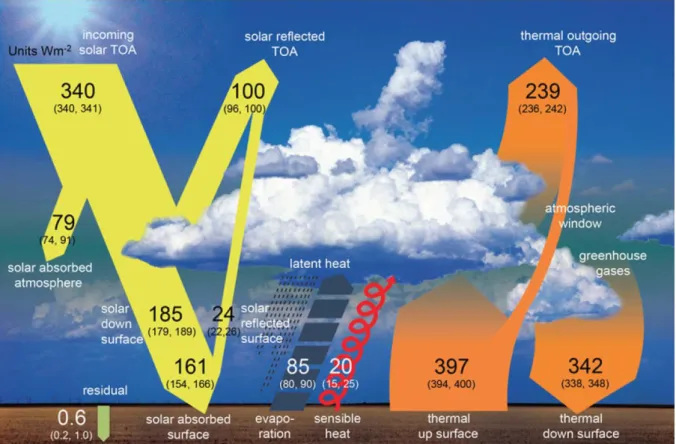
The total instantaneous solar irradiance is 1360.8 Wm-2, or 340 Wm-2 averaged over the
global sphere. Out of the 340 Wm-2 received from the sun, about 100 Wm-2 is reflected by
clouds and atmospheric aerosols (e.g. sulfates, nitrates), leaving 240 Wm-2 to be absorbed by
Earth’s atmosphere (79 Wm-2) and surface (161 Wm-2), as illustrated in Fig. 1-2 (Wild et al.
2013). The planetary albedo (the fraction of SW radiation scattered back to space by the Earth system) is thus 0.29 (Stephens et al. 2015).
FIGURE 1-2: Schematic diagram of the Earth’s global mean energy balance at the beginning of the 21st century.
Large numbers indicate the best estimates and numbers in parentheses the uncertainty range. The figure is extracted from Wild et al. (2013).
In global radiative equilibrium, there is a balance between incoming and outgoing radiation
at TOA. This is almost true, as 239 Wm-2 of LW radiation is emitted from the Earth system at
TOA (Fig. 1-2). The globally averaged TOA net imbalance2 (the net downward heat flux) is 0.6
Wm-2 (Stephens et al. 2012, IPCC AR5 2013). This is how much the Earth system accumulates
heat excess. About 93 % of this excess heat is stored in the ocean, whilst only 1 % in the atmosphere (Loeb et al. 2018).
1
Above the level of unit optical depth, absorption and emission are negligible. Far below this level, the transmissivity of the overlying layer is so small that very little radiation passes through, meaning that most of the radiation has already been absorbed (Wallace and Hobbs 2006).
2
1.1.2 Water Microphysics
The basic concepts of water microphysics presented in this subsection are typically found in basic textbooks on atmospheric science (e.g. Wallace and Hobbs 2006, Ahrens 2013).
Humidity
The relative humidity (RH) of a parcel of air is measured as the ratio of vapor pressure to the saturation vapor pressure (multiplied by 100 for the percentage). The vapor pressure is the pressure exerted by all the water vapor molecules bouncing off the parcel’s interior and the
saturation vapor pressure the pressure exerted by them in a saturated parcel. The saturation
vapor pressure increases with temperature (Clausius-Clapeyron equation, Eq. A1-11), which means that the mass of water vapor to the total mass of all the parcel’s molecules (the specific
humidity) increases with temperature under constant RH. Thermodynamics of Phase Changes of Atmospheric Water
The strong hydrogen bondings between water molecules require much energy to break apart. In order to melt ice into liquid water, the ice must absorb energy from its surroundings to energize the water molecules and weaken the attractive forces between them. The amount of energy required for this phase transition (the heat of fusion) from solid ice to liquid water is
3.34 × 10⁵ J kg-1. Evaporation of liquid water to water vapor then happens in two steps: First,
we must add heat to raise the temperature of the liquid water to 100°C (4.19 × 10⁵ J kg-1).
Second, we must apply additional heat in order for the phase transition from liquid to vapor
(2.25 × 10⁶ J kg-1), referred to as the heat of vaporization. These numbers are taken from
Wallace and Hobbs (2006).
What we just described were endothermic processes in which energy is removed (absorbed) from the surrounding environment. The process can however occur in the other direction as well (i.e. from the gaseous vapor phase to the solid ice phase), in which case the heat of vaporization and heat of fusion are released in the exothermic processes of condensation and
freezing, respectively. The process occurs in both directions in the atmosphere.
These latter exothermic processes are key elements for the process of convection (which is an essential process for tropical heat distribution). When the air becomes supersaturated, atmospheric water vapor condenses onto cloud condensation nuclei and forms clouds. As the vapor condenses it releases its heat of vaporization that has been stored (latent heat) to its surroundings. The warmer surrounding air rises due to increased atmospheric instability and condenses at a higher altitude, thereby raising the cloud height. For temperatures below the 0°C isotherm, ice particles may begin to form on ice condensation nuclei. Because the saturation vapor pressure with respect to ice is less than that of liquid, ice particles grow at the expense of its neighbouring supercooled liquid droplets, when water molecules diffuse from the latter to the former (Wegener 1911, Bergeron 1935, Findeisen 1938). Again, latent heat is released, when less energy is required to keep ice particles in an equilibrium state compared to liquid particles.
Deep convective clouds and systems (e.g. thunderstorms, tropical cyclones) are fueled by the latent heat released when cloud droplets and ice crystals form. Latent heat is the principal energy transport from the surface to the atmosphere in the tropics and responsible for driving the tropical circulation (Sect. 3.1.1.3).
Additionally, liquid and ice phase clouds have important implications on the Earth's radiative balance (as discussed in Sect. 3.1.2.3) by reflecting incoming SW radiation (primarily thick optically clouds) and trapping OLR (primarily high ice clouds).
1.1.3 The Tropical Large-Scale Circulation
This subsection introduces atmospheric circulations in the tropical belt. The information can be found in standard textbooks on atmospheric circulation, like Ahrens 2013 or Holton 2013, which I consulted for details to this description.
The radiative energy balance at TOA is maintained for the closed Earth system, but not for individual regions. The equatorial belt receives the most solar radiation (more than the IR it emits), whilst the poles emit more IR radiation than it receives by the sun. The equatorial energy surplus and polar deficit give rise to a poleward heat transfer within the Earth system, carried by atmospheric winds and ocean currents.
Figure 1-3 illustrates the large-scale circulation in the tropical belt (referred to here as between 30°S to 30°N). From a zonal (latitudinal) perspective, the excessive heating of the equatorial belt forces the surface air to rise, causing surface low pressure there (1-3a). As the warm air rises, it expands and cools. The water vapor it carries condenses into clouds and precipitation, and releases massive amounts of latent heat stored in the water that fuels the ascent by making the air more buoyant.
At the tropopause inversion, the flow is deflected laterally towards the poles. The air grows denser as the air travels poleward due to IR cooling and converging longitudes. Around 30° latitude surface pressure has increased so much that the dense air sinks. As the air descends it is heated by compression, causing a band of semi-permanent high pressure systems in the subtropical region, characterized by clear skies and warm surface temperatures. At the surface level, the air is again deflected laterally. A part of it returns to the equatorial surface low pressure, deflected by the Coriolis force, causing an easterly equatorward return flow, also known as the trade winds. Trade winds in the Northern and Southern hemispheres converge at the equator along a boundary referred to as the Intertropical Convergence Zone (ITCZ), characterized by strong ascent and vigorous convection. This atmospheric cell between the
equator and 30° latitude is referred to as the Hadley cell3 (Fig. 1-3a).
Superimposed on the zonally distributed Hadley cell, are zonally asymmetric atmospheric circulations (1-3b), caused by longitudinal variations in sea surface temperature. The easterly trade winds drag the equatorial surface water westward, concentrating the warm surface waters off the east coasts of tropical land masses and raising the sea level there, whilst lowering the sea level off the west coast of tropical continents and promoting upwelling of cooler ocean waters there. This is best seen in the tropical Pacific (Fig. 1-3c), with the Pacific Warm Pool region in the west (covering Oceania and usually extending into the Indian Ocean) and cold waters off the west coast of Peru.
3
The Hadley cell is named after the English meteorologist George Hadley. For more information about the atmospheric general circulation (e.g. the Ferrel cell between 30° and 60° or the Polar cell between 60° and 90°), the reader is referred to standard textbooks on atmospheric physics (e.g. Wallace and Hobbs 2006, Ahrens 2013, Holton 2013)
FIGURE 1-3: Illustration of the tropical large-scale circulation. a) The Hadley cell, the meridional tropical
circulation. b) The zonal tropical large-scale circulation. c) The Pacific Walker circulation (as also located in b). Notations “H” and “L” stand for surface high and low pressures respectively. Subplot c is extracted from Ahrens 2013 (reprinted from Cengage Learning) and subplot b from NOAA Climate.gov. (accessed on May 27, 2020):
https://www.climate.gov/news-features/blogs/enso/walker-circulation-ensos-atmospheric-buddy
Thus, tropical atmospheric processes are subject to both dynamic (linked to atmospheric circulation) and thermodynamic (linked to temperature) (Sect. 1.1.2) influences, where cloud formation is sensitive to both albeit predominantly to the former (Bony et al. 2004). The large-scale circulation (dynamical) can be observed by measures of vertical velocity. The most common proxy for large-scale circulation is perhaps the vertical pressure velocity at the 500 hPa level (e.g. Su et al. 2011, Konsta et al. 2012, Vaillant de Guélis et al. 2017, Chepfer et al. 2019), which is the parameter that I employ in Ch. 3 as a proxy for the tropical large-scale circulation.
1.2 Radiation and the Water Cycle
This section discusses current knowns and unknowns of the interactions of radiation and the water cycle. Sect. 1.2.1 introduces the concept of radiative forcing and climate feedbacks. It is with respect to the current principal uncertainties for solving the feedback equation that my work is motivated, i.e. the rate of change of water cycle variables with surface temperature. The principal climate feedbacks are separated into clear-sky feedbacks (Sect. 1.2.2) and cloud feedbacks (Sect. 1.2.3) and explained in more detail in these sections.
1.2.1 Radiative Forcing and Climate Feedbacks
The radiative balance at TOA has been perturbed by a radiative forcing F, induced by an anthropogenic increase in greenhouse gas concentrations (IPCC AR5, 2013), which gives rise to a net downward radiation at TOA (ΔR) and an accumulation of energy in the Earth system that will ultimately force the climate to change and establish a new equilibrium surface
temperature TS (Rose and Rayborn 2016). The climate feedback formalism assumes that
changes in radiative flux are proportional to changes in surface temperature. Then, the global energy imbalance at TOA can be written
∆𝑅 = 𝐹 + 𝜆∆𝑇𝑠 (E1-1)
where the constant of proportionality λ is the total climate feedback parameter (Charney et al. 1979), assumed to be timescale-invariant (Gregory et al. 2004). Eventually, the Earth system will adjust to this imbalance, as ΔR goes to zero when the warmer planet emits more energy to space (Rose and Rayborn 2016, Goosse et al. 2018). The adjustment time differs however between the Earth system’s components (atmosphere, ocean, continent, cryosphere, etc.), and a new equilibrium temperature is not achieved until all components have adjusted to the forcing.
With ΔR = 0, the ultimate change in global surface temperature ΔTS due to the radiative forcing
is characterized by:
𝐹 = −𝜆∆𝑇𝑠 (E1-2)
The assumption of linear dependence on ΔTS implies that the total climate feedback parameter
can be decomposed into individual additive components, each one representative of a different radiative process internal to the Earth system (Wallace and Hobbs 2006):
𝜆 = ∑ 𝜆𝑗
𝑗
(E1-3)
If we insert E1-3 in E1-2 and divide by ΔTS, we can expand the expression and see that the
change in radiative flux with surface temperature is both sensitive to atmospheric water cycle
variables Yj and their responses to changes in surface temperature:
𝑑𝐹 𝑑𝑇𝑠 = 𝜕𝐹 𝜕𝑇𝑠+ ∑ 𝜕𝐹 𝜕𝑌𝑗 𝑑𝑌𝑗 𝑑𝑇𝑠 𝑗 (E1-4) where the last term can be expanded to
𝑑𝑌𝑗 𝑑𝑇𝑠 = 𝜕𝑌𝑗 𝜕𝑇𝑠+ ∑ 𝜕𝑌𝑗 𝜕𝑌𝑘 𝑑𝑌𝑘 𝑑𝑇𝑠 𝑘 (E1-5)
on account of many of the atmospheric water cycle variables Y being dependent on each other
(e.g. the dependence of clouds Yj on humidity Yk). From these expansions we can think of a
feedback factor as the sensitivity of a variable to some meteorological predictor, scaled by the change of the control predictor’s response to climate change.
Of these terms, the sensitivities of the TOA radiative fluxes to changes in humidity and clouds (dF/dY) are fairly well known as they can be reliably estimated from radiative transfer computations (e.g. Liou 2002). In contrast, responses of the water cycle variables to climate
warming (dY/dTS) are more uncertain. First order uncertainties are related to how the individual
water cycle variables vary with surface temperature (dYj/dTS, E1-4), and second order
uncertainties to how the water cycle variables vary with each other (dYj/dYk, E1-5).
The total climate feedback parameter λ is usually decomposed into a sum of five terms: 1) the Planck feedback, 2) the water vapor feedback, 3) the lapse rate feedback, 4) the cloud feedback, and 5) the albedo feedback (Dufresne and Bony 2008):
𝜆 = 𝜆𝑃+ 𝜆𝑊𝑉 + 𝜆𝐿𝑅+ 𝜆𝐶+ 𝜆𝛼 (E1-6)
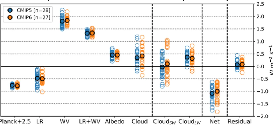
Feedbacks 1 to 44 will be described next in sections 1.2.2 and 1.2.3. Figure 1-4 below shows
the ensemble mean global radiative feedback estimates from CMIP5 and CMIP6 models. Evidently, the largest intermodel spread is seen for the cloud feedbacks. In fact, cloud responses
to climate change are highlighted by the Global Energy and Water cycle Exchanges (GEWEX5)
as one of the grand challenges and a major uncertainty for climate sensitivity estimates and modelled circulation (Bony et al. 2015).
4
The albedo feedback (5), also called the ice-albedo feedback, is not relevant for the tropical region.
5
GEWEX is one of the core projects under the World Climate Research Programme (WCRP) dedicated to understanding Earth’s water cycle and energy fluxes at and below the surface and in the atmosphere:
FIGURE 1-4: Estimates of global radiative feedbacks from abrupt-4xCO2 experiments in CMIP5 (blue) and
CMIP6 (orange), a) relative to constant specific humidity and b) relative to constant relative humidity. The subplots are extracted from Zelinka et al. (2020).
1.2.2 Clear-Sky Feedbacks
The Planck feedback (e.g. Hansen et al. 1984) is the strongest negative climate feedback and results from the Planck function (Eq. A1-1), where the blackbody radiation of an object is a function of its temperature. This is the most fundamental climate feedback, simply stating that the warmer the Earth, the more it radiates.
Following the Clausius-Clapeyron equation (EA-11), specific humidity increases
approximately exponentially with temperature (at a rate of about 6 to 7 % K-1), under the
assumption of constant relative humidity (e.g. Raval and Ramanathan 1989, Allan 2012, Dewey
and Goldblatt6 2018). The higher concentrations of water vapor increase the greenhouse effect
and accelerates the warming. This water vapor feedback (Held and Soden 2000) is the strongest warming climate feedback (e.g. Soden and Held 2006, Dessler 2013, Ingram 2013).
The lapse rate feedback is due to vertically non-uniform atmospheric heating. If the upper troposphere warms more than the lower troposphere, the lapse rate decreases and the emission to space moves closer to the emission from Earth’s surface. Thus, the greenhouse effect is less efficient, and the sign of this feedback is negative. The lapse rate feedback is robustly negative in the tropics where the temperature profile follows the moist adiabatic lapse rate, but can be
6
Dewey and Goldblatt 2018 observed decreasing OLR for surface temperatures in excess of ~298 K, whilst a continued nonlinear increase in column integrated water vapor.
positive in high latitudes in the presence of stable stratification that suppresses vertical mixing, thereby confining the warming to a thin near-surface layer (Soden and Held 2006, Pithan and Mauritsen 2013, Goosse et al. 2018).
But the lapse rate is a function of RH as well, where the non-uniform tropospheric heating can change as a result of non-uniform change in RH with warming. Because the radiative effect (IR absorption) of water vapor is roughly proportional to the logarithm of its relative humidity (Allan et al. 1999, Roca et al. 2000), the radiative impact of a change in water vapor concentration is greatest (smallest) at initially low (high) relative humidities as illustrated in Fig. 1-5 below. A change in the lapse rate can thus result from only a small increase in initial upper tropospheric relative humidity (which is significantly drier than the lower troposphere).
FIGURE 1-5: Sensitivity of the change in clear-sky OLR with tropospheric RH (dOLR/dTRH) to the mean
tropospheric RH from the European Centre for Medium-Range Weather Forecasts ReAnalysis project over the time period 1979 to 1993. The figure is extracted from Allan et al. (1999).
Because these clear-sky feedbacks (Planck, lapse rate, water vapor) are not independent of each other, the effects of them are often combined assuming constant relative humidity, as advocated by Held and Shell (2012). An example of this is seen in Fig. 1-4 above, where the
ensemble mean values of these feedbacks are reduced from about –3.2 W m-2 K-1, –0.5 W m-2
K-1 and +1.8 W m-2 K-1 respectively, to about –1.8, –0.1 and +0.05 W m-2 K-1 (Caldwell et al.
2016, Zelinka et al. 2020). This repartitioning limits the spread in general circulation model (GCM) projections around the ensemble mean (Ingram 2013), reduces the covariance between the lapse rate and water vapor feedbacks (Caldwell et al. 2016), and avoids dealing with feedback computations relative to unrealistic supersaturated base states (Held and Shell 2012).
1.2.3 Cloud Feedbacks and Radiative Effects
In cloudy scenes, two competing radiative effects stand against each other; the SW and the LW. At TOA, the cloud radiative effect (CRE) is defined as the difference between the downwelling and upwelling radiative fluxes in all-sky situations minus the difference in clear-sky situations (Matus and L’Ecuyer 2017):
𝐶𝑅𝐸 = (𝐹↓− 𝐹↑)
𝑎𝑙𝑙 𝑠𝑘𝑦 − (𝐹
↓− 𝐹↑)
𝑐𝑙𝑒𝑎𝑟 𝑠𝑘𝑦 (E1-7)
The shortwave cloud radiative effect (SWCRE) is due to the high albedo of clouds (Stephens et al. 2015). The SWCRE therefore has a cooling effect on the Earth system as it prevents solar radiation from being absorbed. The SWCRE is sensitive to the size of the reflective droplets (liquid cloud droplets are smaller and closer than ice crystals to SW wavelengths), and the condensed water amount (optically thick clouds reflect more than optically thin clouds) (Stephens and Tsay 1990, Hogan et al. 2003, Henderson et al. 2012).
Clouds also absorb LW radiation. Effectively so in the 8 and 11 μm range, thereby closing the atmospheric window (Wallace and Hobbs 2006, Ahrens 2013). The longwave cloud radiative effect (LWCRE) is due to clouds’ ability to decrease the OLR, by absorbing surface emitted IR radiation at their bases and emitting OLR from their tops. Because temperature decreases with altitude in the troposphere, the temperature at the cloud top is colder than the surface temperature, so OLR emitted from clouds is less than OLR emitted from Earth’s surface. Hence, the LWCRE has a warming effect and the higher the cloud altitude, the colder the emission temperature, and the greater the difference between OLR emitted at cloud top and Earth’s surface.
The SWCRE and LWCRE always compete where clouds are present. Because warm low liquid clouds have higher albedo than cold high ice clouds, and because their cloud tops are not much colder than the surface (~10 degrees), the net CRE is dominated by the stronger SWCRE. However, for high ice clouds, the warming LWCRE is considerably more important for the net CRE.
The SW and LW cloud feedbacks are then the changes in SWCRE and LWCRE at TOA with surface warming (Vaillant de Guélis et al. 2018). In the tropics, the principal regions of interest for the SW cloud feedback are tropical subsidence regions off the west coast of continents characterized by low clouds (often referred to as the stratocumulus regions), whilst the LW cloud feedback is interesting for convective regions. Figure 1-6 below shows global mean cloud feedbacks in CFMIP1 and CFMIP2 models. It shows that the LW cloud feedback (red) is dominated by changes in cloud cover (“Amount” in Fig. 1-6), altitude and optical depth, whilst the SW cloud feedback (blue) is only sensitive to cloud cover and optical depth.
The LW cloud feedback is positive in models (e.g. Zelinka et al. 2013, 2016, 2020, Ceppi and Gregory 2017) primarily due to rising cloud altitudes of high clouds with surface warming (Fig. 6a,b). The positive sign is only partly offset by decreasing high cloud cover (Fig. 1-6a,b). Rising cloud altitudes and dropping cloud temperatures have also been reported in process-oriented observational studies. For example, Igel et al. (2014), observed rising anvil bases and decreasing cloud-top temperatures measured by CloudSat with warmer surface
temperature. However Vaillant de Guélis et al.7 (2018) showed that the LW cloud feedback is negative in observations by CALIPSO and CERES, due to decreasing opaque cloud cover with surface temperature. The decreasing opaque cloud cover induces a negative LW cloud feedback whose magnitude is more than twice the positive LW cloud feedback induced by rising opaque cloud altitudes. This is an important result as it shifts (i) the sign of the total observed LW cloud feedback from positive to negative and (ii) the principal determining variable from opaque altitude to cover. How the anvil width changes with surface warming is diverging in previous observational studies (e.g. Lindzen et al. 2001, Rapp et al. 2005, Su et al. 2008, Igel et al. 2014), likely due to different study regions, evaluation methods and observational instruments (Hartmann and Michelsen 2002).
FIGURE 1-6: Global mean (red) LW, (blue) SW, and (black) net cloud feedbacks decomposed into amount,
altitude, optical depth, and residual components for (a) all clouds, (b) non-low clouds only, and (c) low clouds only. Open symbols are for CFMIP1 models and filled symbols are for CFMIP2 models. Multimodel mean feedbacks are shown as bars. The figure is extracted from Zelinka et al. (2016).
7
Vaillant de Guélis et al. (2018): CALIPSO, CERES EBAF, monthly global means over ocean surfaces, 2008-2014
Like the LW cloud feedback, the SW cloud feedback is also positive in models (Fig. 1-4, 1-6a). The positive sign is explained by decreasing tropical marine boundary layer cloud cover with SST, which induces a warming due to more SW absorption (1-6c) (Ceppi and Gregory 2017, Zelinka et al. 2012, 2020). The total SW cloud feedback is only partly off-set by increasing cloud optical depth with surface warming, which poses a range of negative SW feedbacks (Fig. 1-6, Zelinka et al. 2016). There seems to be a general consensus on the sign of the rate of change of marine boundary layer cloud cover and SST between model and observational studies (as observed in e.g. Zhai et al. 2015), but the exact rate of change of this decrease is not known and is the principal reason for intermodel spreads (Figs. 1-4, 1-6). The sensitivity of the marine boundary layer cloud cover to SST is identified as an emergent
constraint (Focus Box 1) and a key uncertainty for climate models (Bony and Dufresne 2005,
Ceppi et al. 2017).
A key feature for the overall decrease in marine boundary layer cloud cover with SST seems to be a greater moisture contrast between the boundary layer (BL) and the free troposphere (FT) with warmer surface temperatures that can arise either due to enhanced surface latent heat flux, or through greater surface evaporation (Kamae et al. 2016). Regardless, the moisture contrast between the BL and FT means a greater vertical gradient of moist static energy that causes enhanced vertical mixing and drying at the capping inversion, and an effectively deeper BL with horizontally smaller clouds (Brient and Bony 2013, Myers and Norris 2013, Wood and Bretherton 2016).
FOCUS BOX 1: EMERGENT CONSTRAINTS
Is there a way to decide which quantities of the current climate are relevant for climate change? Emergent constraints (Klein and Hall 2015) answer this question by examining the collective behavior that emerges unexpectedly in climate model ensembles. They are physically explainable empirical relationships between characteristics of the current climate and long-term climate prediction that emerge in collections of climate model simulations (Klein and Hall 2015).
Klein and Hall (2015) identifies the following three potential emergent constraints for cloud feedbacks: (1) low-level cloud optical depth, (2) subtropical marine low-level cloud cover, and (3) lower tropospheric mixing. These are listed in the inserted table below:
The study of low cloud cover with SST is motivated by recent work in e.g. Klein et al.
(2017) and Zelinka et al.8 (2020). They found that the sensitivity of low cloud cover to SST was
small compared to other cloud controlling factors (estimated inversion strength, RH, pressure velocity), but that the change in SST with unit global warming was about 10 times greater than the change in any of the other cloud controlling factors, making the predicted change in low cloud cover per unit global warming most sensitive to SST.
On the global scale, the Earth system can be thought of as a closed system, but on shorter timescales, local and regional states are dominated by e.g. seasonal or diurnal scale processes. Knowing that different components of the Earth system adjust to a climate forcing on different timescales, and that different atmospheric processes and mechanisms are important on different timescales, how can we assume that the individual feedback terms are timescale-invariant? Klein et al. (2017) assumed sensitivities of the low cloud cover to various cloud controlling factors to be constant in time, but ended their work with a thorough discussion on the validity of the assumption of timescale invariant feedback terms.
1.3 Principal Hypotheses About the Tropical Atmospheric Water
Cycle’s Response to Surface Warming
The previous section discussed changes in clear-sky and cloudy-sky feedbacks separately. This section discusses the collective response of the atmospheric water cycle to SST over the full tropical belt, including both clear-sky and cloud feedbacks. Here I also explain the most discussed hypotheses concerning the tropical atmospheric water cycle’s response to surface warming, with special emphasis on the iris and Fixed-Anvil Temperature (FAT) hypotheses that are investigated in this work.
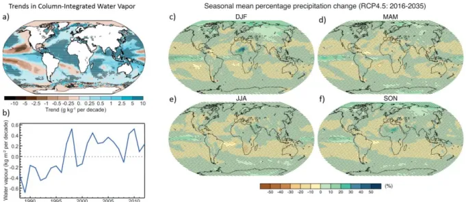
The hydrological cycle is expected to intensify, with increasing surface evaporation following the warming, making more atmospheric water available for precipitation. Globally, already wet regions (precipitation rate > evaporation rate) grow wetter, whilst dry regions (evaporation > precipitation) become even drier in a nonuniform response of the global water cycle referred to as “wet-get-wetter” and “dry-get-drier” trend (IPCC AR5, 2013). It is illustrated in Fig. 1-7 by observed trends in surface specific humidity over oceans (a) and predicted precipitation changes in the RCP4.5 scenario (c-f).
Hypotheses regarding the responses of the tropical region to surface warming discuss an intensified hydrological cycle, characterized by a narrowing of the ascending branch of the Hadley circulation with stronger updrafts in moist convective regions and horizontally broader clear-sky subsidence regions, as illustrated in the conceptual schematic from Su et al. (2017) based on ensemble means of climate model simulations under global warming (Fig. 1-8).
8
Zelinka et al. (2020) compared results of climate sensitivity and radiative feedbacks in CMIP5 and CMIP6 models.
FIGURE 1-7: a) Trends in column-integrated water vapor observed by the Special Sensor Imager over ocean
surfaces over the period 1988 to 2012. b) Global annual average column-integrated water vapor over ocean surfaces relative to the 1988 to 2007 average. c-f) Seasonal multi-model ensemble mean of 42 CMIP5 models for projected changes in precipitation (%) over the period 2016 to 2035 relative to 1986 to 2005 under RCP4.5. The figures are extracted from IPCC AR5 (2013).
FIGURE 1-8: Schematic of the tightening of the Hadley circulation in a warmer climate. Light colors represent
the current climate and dark colors a warmer climate. The figure is extracted from Su et al. (2017).
The intensified tropical hydrological cycle is fueled by greater moisture supply from enhanced surface evaporation and horizontal moisture convergence that enable greater latent heat release in the updraft. The stronger updrafts cause convective anvils to rise, but also greater precipitation efficiency, leaving fewer hydrometeors to build up the anvil cloud, effectively shrinking the horizontal extent of the anvil and allowing more OLR to be emitted to space in the clear skies outside of the convective clouds (Su et al. 2017).
This reasoning is the basic theory for the iris hypothesis (first postulated by Lindzen9 et al. 2001, and subsequently revised in e.g. Fu et al. 2002, Hartmann and Michelsen 2002, Lin et al.
2002, 2004, 2006, Su et al. 2008, Mauritsen and Stevens10 2015.) in which precipitation
efficiency increases with SST, leading to smaller convective anvils and effectively more OLR as fewer hydrometeors are left to build these (Fig. 1-8). Radiatively, the increase in OLR is balanced by an increase in latent heat release due to greater convective precipitation efficiency. To a first approximation, the iris hypothesis compares the extent of the tropical moist and dry regions. It received its name from the adaptive behavior of the system to open (close) to allow for more (less) OLR to be emitted to space with warmer (colder) surface temperature, in much the same way as the eye’s iris opens/closes to light changes (Lindzen et al. 2001). This thinking is in line with Pierrehumbert (1995) who suggested a regulation by the area of large-scale subsidence regions (radiator fins), in which the clear-sky GHE is determined by the water vapor feedback. Such radiator fins (illustrated in Fig. 1-8) are consistent with broader clear-sky subsidence regions with surface warming.
Within a stronger updraft, it is possible that SW reflection increases, which could explain
the thermostat hypothesis, proposed by Ramanathan and Collins11 (1991), where thicker cirrus
anvils act like a thermostat regulating the amount of SW radiation that can be absorbed by the
surface. Observational support for this hypothesis was found in e.g. Lebsock et al.12 (2010) and
Igel et al.13 (2014).
In the Fixed-Anvil Temperature hypothesis (FAT), first presented by Hartmann and Larson (2002) (and subsequently assessed in a number of papers, e.g. Zelinka and Hartmann 2010, 2011, Seeley et al. 2019), cloud altitudes rise in response to surface temperature increase. They rise in such a way that they stay at the same temperatures as before the warming, which means that the temperature at the anvil detrainment level remains constant, making the anvil emission temperatures and the OLR independent of surface temperature. The altitude of anvil detrainment (convective outflow) occurs at the altitude where radiative cooling decreases most rapidly with height, which is where the saturation vapor pressure of water vapor becomes so low that water vapor no longer has a significant effect on the emitted radiation.
9
Lindzen et al. (2001) used cloud observations from the Japanese Geostationary Meteorological Satellite-5 over the western Pacific (30°S to 30°N and 130°E to 170°W).
10 Mauritsen and Stevens (2015) found that inclusion of an iris effect in the ECHAM6 GCM brought simulated
equilibrium climate sensitivity closer to observed values.
11 Ramanathan and Collins (1991) used radiation data from the Earth Radiation Budget Experiment and sea surface
temperature from weather satellites and ships over the time period 1985 to 1989, including the El Niño event in 1987. They found that cirrus anvils were thicker and their SW reflectivity anomaly higher over the warmest sea surface temperatures during the 1987 El Niño event.
12
Lebsock et al. (2010) found positive correlations between precipitation rate (AMSR-E) and high-cloud reflectivity (CERES-EBAF) in the tropics.
13
Igel et al. (2014) observed physically thicker cloud anvils and increasing ice water path in convective systems derived from CloudSat observations.
FOCUS BOX 2: SUPER-GREENHOUSE EFFECT
The super-greenhouse effect (SGE, e.g. Hallberg and Inamdar 1993, Raval and Ramanathan 1989) refers to those tropical locations where the Planck function fails to stabilize the climate (Stephens et al. 2016), which is effectively where OLR decreases with SST. Following the equations outlined in Valero et al. (1997), the greenhouse effect G can be expressed as:
𝐺 = 𝜀𝜎(𝑆𝑆𝑇4) − 𝑂𝐿𝑅
Where ε is the emissivity of the Earth’s surface and σ the Stefan-Boltzmann constant. The SGE is thus present when:
𝑑𝐺
𝑑𝑆𝑆𝑇 > 4𝜀𝜎(𝑆𝑆𝑇
3)
Dewey and Goldblatt (2018) find that the decrease in OLR with SST occurs for SSTs > 298 K (Fig. Ba). Column moistening by deep convection in cloudy regions and advection of moisture in clear-sky regions, increases the proportion of OLR that originates from the cold high troposphere rather than the warm surface.
FIGURE B: (a) Observational OLR dependence on SST, and OLR output for various humidity values. The red
dashed line is the mean, and the black circles correspond to the panels in (b). (b) Spectra of thermal emission altitude. The bottom four panels are the surface temperatures and RH where the observational OLR intersects model curves, and the top two panels are at higher surface temperatures, both with 100 % RH. The background color indicates the atmospheric temperature, and the white line is the altitude at which optical depth is unity. The figure is extracted from Dewey and Goldblatt (2018).
Bony et al.14 (2016) revisited both the iris and the FAT hypotheses using three GCMs and proposed the idea of a “stability iris mechanism” that links the two, where the detrainment is controlled by stability (the ratio of the radiative cooling to vertical velocity). Tropical stability (σ) is balanced by radiative cooling (Q) and radiatively driven subsidence rate (ω): σ = Q / ω (Allan 2012). Greater atmospheric moisture associated with warmer temperatures moves the environmental lapse rate closer to the moist adiabatic lapse rate, thus increasing the atmospheric stability and diminishing the radiative cooling and the subsidence rate needed to balance it, resulting in less convective outflow.
1.4 Present Day Limitations with Observations and Models
1.4.1 Observational Limitations
Issues that deal with circulation, cloud and climate relations require analyses of observations to test for theories and hypotheses. These must be able to accurately sample the key water cycle variables with high temporal and spatial resolution over the full tropical belt, and must cover a long enough time period to account for natural and interannual variability – with the dominant tropical interannual variability being the El Niño-Southern Oscillation.
That said, observations are snapshots of reality that require analysis and theories to explain what they show. The reason is that all variables change together in observations, and they can therefore not be used to study causality. Nor can they be used to study isolated physical processes or mechanisms that require all other aspects of the atmosphere to be held fixed.
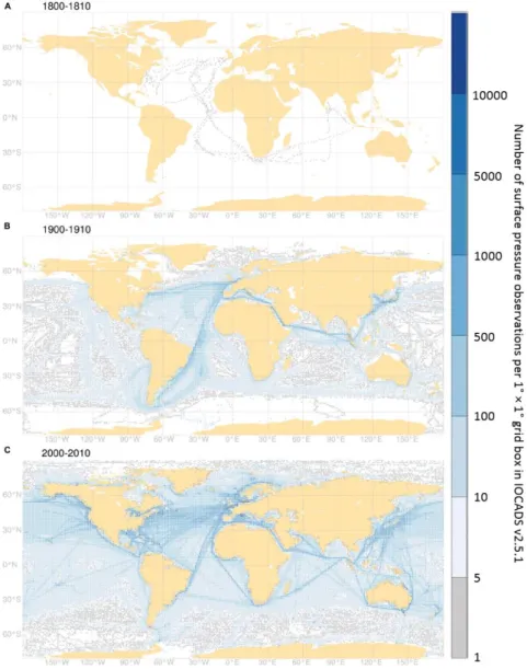
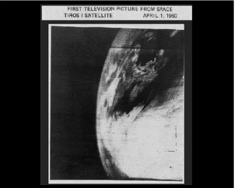
For a long time, the observational coverage was limited to land stations or ship tracks at sea. For that reason the observational coverage is much denser and continuous records extend much further back in time over land than over oceans. Fig. 1-9 shows the number of observations made in oceanic 1° × 1° grid boxes following ship tracks over the first decade in the 19th, 20th and 21st centuries. The top figure shows that the tropical Pacific Ocean was completely unobserved during the 19th and early 20th century. It took until the dawn of the satellite era and the launch of the first weather satellites Vanguard 2, Explorer-6, Explorer-7 and TIROS 1 (Television InfraRed Observational Satellite) in the late 1950s and early 1960s (Capderou 2014) for atmospheric observations to be possible over ocean surfaces outside of ship tracks and unpopulated land surfaces. These satellite observations provided the first global views of the atmospheric water cycle and TOA radiative fluxes. Fig. 1-10 below shows the first image of the Earth taken by a weather satellite. This image was taken by the TIROS 1 satellite, whose objective was to test experimental television techniques designed to develop a worldwide
meteorological satellite information system (
https://airandspace.si.edu/collection-objects/tiros-meteorological-satellite/nasm_A19650289000, accessed September 8, 2020). The satellite carried two television cameras, one of low and a second of high resolution.
14
FIGURE 1-9: Data counts per 1° × 1° latitude, longitude of surface pressure observations by ships in the
International Comprehensive Ocean-Atmosphere Data Set, used by the National Oceanic and Atmospheric Administration and European Centre for Medium-Range Weather Forecasts 20th century reanalyses, for three selected time periods: (A) 1800–1810, (B) 1900–1910, and (C) 2000–2010. The figure is extracted from Smith et al. (2019).
Back then, satellites were equipped with passive sensors that could not observe the detailed vertical structure of the atmosphere, which is perhaps why previous work only studied one vertical range (e.g. Ross et al. 2002, Gettleman et al. 2006, Läderch and Raible 2013). Detailed observations could be made in field campaigns with radiosondes or aircraft measurements, but as these only observed a local restricted region, they under sampled the tropics and missed the large-scale context. It was not until the turn of the millennium that active sensors (e.g. lidars and radars) were mounted onboard satellites, providing means of detailed observations of global coverage. By now, these instruments have been in use long enough to account for natural variability and detect significant trends.
FIGURE 1-10: The figure shows the first image taken of the Earth by a weather satellite, the TIROS 1 satellite.
It is extracted from NASA (accessed September 8, 2020):
https://www.nasa.gov/vision/earth/features/bm_gallery_3.html
1.4.2 Model Limitations
In contrast to observations, climate models are very useful for tracking processes as well as for projections of historical and future climate scenarios. They are rooted to their best ability in physical laws, but all equations cannot be solved analytically, which is why the models must rely on numerical estimations and parameterizations.
However, not all processes are described equally in all models, nor do they all make the same assumptions. This leads to significant intermodel spreads of key results with a wide range of projections (as illustrated in Figs. 1-4 and 1-6) when the models do not converge towards a single behavior (e.g. Andrews et al. 2012, Vial et al. 2013, Po-Chedley et al. 2018, Zelinka et al. 2016, 2020). This is particularly concerning for feedback mechanisms and climate sensitivity that must be computed by numerical models.
Still, as computer power increases and more data storage is made available, climate model performance is constantly advancing, with more accurate predictions of higher resolutions and longer records.
1.5 Principal Science Questions
Given that the primary feedback uncertainties are derived to uncertainties in how moisture and clouds vary with surface warming, this work aims to improve on our understanding of the relationships between the RH profile and cloud characteristics with SST.
1.5.1 Focus on the Instantaneous Timescale and Large-Scale Regimes
Short and local scales are where we come the closest to observing covariations of variables of interest. Instantaneous observations of one or two of the key water cycle variables (moisture, clouds, precipitation) have been made in the past, but the study in Chapter 3 observes instantaneous covariations of the RH profile and cloud cover with SST over the full tropical belt and under the influence of the large-scale circulation. The principal questions asked are:
• Do RH and cloud cover vary differently with SST under large-scale ascent and descent? • Do RH and cloud cover vary differently with SST in the presence and absence of
precipitation?
• Do low liquid and high ice cloud covers vary differently with SST?
• Does the RH profile vary differently with SST in the vicinity of low liquid clouds and high ice clouds?
1.5.2 Focus on Different Temporal and Spatial Scales
Chapter 3 studies covariations of some of the key components of the tropical atmospheric water cycle on the instantaneous grid box scale. It is thus restricted to one temporal scale and one spatial scale. In contrast, the study in Chapter 4 assesses the dependence of the water cycle variables’ covariations and responses to SST warming on the choice of temporal and spatial scale by observing them on four different timescales (daily, monthly, seasonal, annual), as well as in both spatially global values and more process-oriented grid box values.
Spatial and temporal scales are not independent of each other, as the larger the atmospheric system/phenomenon, the longer its expected lifespan or the adjustment time to changes for the components and variables it interacts with (e.g. Orlanski 1975, Steyn et al. 1981). Process-oriented studies are best executed on small and short spatial and temporal scales, whilst climatological long-term trends are most relevant on the global scale, as climate change is constrained by the global energy budget and the net radiative flux at TOA. Time-varying climate predictions have previously been made with models (e.g. Armour et al. 2013, Gregory and Andrews 2016), but I am unaware of observational studies that deal with the sensitivity of the atmospheric water cycle to surface temperature across timescales.
The principal questions asked in this study are:
• How do RH and cloud cover, altitude, temperature vary with SST on different timescales? This question targets the principal uncertain terms in the feedback equation. • How does the low cloud cover vary with SST on different timescales? This question is
central to the SW cloud feedback.
• How do high ice cloud characteristics (cover, altitude, temperature) vary with SST over the warmest waters? This question is central to the LW cloud feedback and relates to both the iris and FAT hypotheses.
• How do cloud characteristics covary and how do they vary with the RH profile? These are the second order uncertain terms in the feedback equation.
Secondary questions ask if the signs and magnitudes of these rates of changes are robust across timescales? These are novel questions from an observational perspective.
1.5.3 Dataset Objective
Answers to the science questions listed above require a comprehensive observational dataset. In Chapter 2, I build a dataset of observational diagnostics on a regular grid of 1° × 1° spatial resolution that can be directly relatable to climate studies. This resolution is a common standard today, which roughly translates into 100 km × 100 km in the tropics.
1.5.4 Manuscript Structure
To answer these questions, I have built a synergistic dataset of collocated instantaneous observations of the tropical atmospheric water cycle. Chapter 2 presents these observational products and the instrument payloads from which they are retrieved. In Chapter 3, I assess how the RH profile and cloud cover varies with SST on the instantaneous timescale under the influence of the tropical large-scale circulation (i.e. the questions asked in Sect. 1.5.1). In Chapter 4, I assess the dependence of the water cycle variables’ covariations and responses to surface warming on the choice of temporal and spatial scale by observing them on four different timescales (daily, monthly, seasonal, annual), as well as in both spatially global values and more process-oriented grid box values (the questions asked in Sect. 1.5.2). I end this manuscript by a concluding chapter, where I have summarized the answers to the principal science questions and put the results in perspective.
Chapter 2
2 The Synergistic Dataset
2 The Synergistic Dataset ... 29 2.1 Introduction to the Dataset ... 30 2.2 Relative Humidity from SAPHIR ... 32 2.2.1 The Megha-Tropiques Mission... 32 2.2.2 The SAPHIR Microwave Radiometer ... 34 2.2.2.1 Microwave Sounding of Water Vapor ... 34 2.2.2.2 The SAPHIR Sounder ... 35 2.2.3 RH Profile Retrievals from SAPHIR ... 36 2.2.4 The Gridded RH Product... 37 2.2.5 Advantages and Limitations with SAPHIR ... 38 2.2.5.1 Advantages ... 38 2.2.5.2 Limitations ... 39 2.3 Cloud Characteristics from GOCCP ... 40 2.3.1 The A-Train Constellation... 40 2.3.2 The Lidar CALIOP ... 41 2.3.2.1 Lidar ... 41 2.3.2.2 CALIOP ... 42 2.3.3 Single Profile GOCCP-OPAQ... 42 2.3.4 The Gridded Cloud Product... 45 2.3.5 Advantages and Limitations with GOCCP... 47 2.3.5.1 Advantages ... 47 2.3.5.2 Limitations ... 47 2.4 Near-Surface Precipitation from the CloudSat 2C-PRECIP-COLUMN Product ... 47 2.4.1 CloudSat’s Cloud Profiling Radar ... 47 2.4.1.1 Radar ... 47 2.4.1.2 The Cloud Profiling Radar ... 49 2.4.2 Single Column: Retrievals from the 2C-PRECIP-COLUMN Product ... 49 2.4.3 The Gridded Precipitation Product ... 51 2.4.4 Advantages and Limitations with CloudSat 2C-PRECIP-COLUMN ... 53 2.4.4.1 Advantages ... 53 2.4.4.2 Limitations ... 53
2.5 Surface Temperature and Vertical Pressure Velocity from ERA5 ... 54 2.5.1 ERA5 Reanalysis ... 54 2.5.2 The ERA5 Variables Used in This Work ... 54 2.5.2.1 Skin Surface Temperature ... 54 2.5.2.2 Atmospheric Vertical Pressure Velocity ... 55 2.5.3 Advantages and Limitations with ERA5 ... 56 2.5.3.1 Advantages ... 56 2.5.3.2 Limitations ... 57 2.6 Satellite Collocations ... 57
2.1 Introduction to the Dataset
Better understanding of how the key tropical atmospheric water cycle variables (temperature, moisture, clouds, precipitation, radiation) covary under climate warming lacks a comprehensive observational view. As discussed in Ch. 1, previous observational work typically did not observe the detailed vertical structure of the tropical atmospheric water cycle and the instantaneous covariations between its key variables (moisture, clouds, precipitation). Or if they did, they under sampled the tropical region and therefore missed the large-scale context.
To answer the science questions asked in Ch.1, I have built a synergistic dataset of collocated instantaneous observational products, encompassing the atmospheric water cycle over the tropical belt (30°N to 30°S) on a 1° × 1° spatial grid. This chapter presents these observational products and the instrument payloads from which they are retrieved, as well as their principal advantages and limitations. Each instrument payload and the variables retrieved from it, is the focus of one section.
The dataset includes:
• the relative humidity profile, observed by the passive microwave radiometer SAPHIR (Sounder for Atmospheric Profiling of Humidity in the Intertropics by Radiometry) onboard the Megha-Tropiques satellite (presented in Sect. 2.2)
• cloud characteristics, observed by the lidar CALIOP (Cloud-Aerosol Lidar with Orthogonal Polarization) onboard the CALIPSO (Cloud-Aerosol Lidar and Infrared Pathfinder Satellite Observations) satellite (presented in Sect. 2.3)
• near-surface precipitation, observed by the cloud profiling radar (CPR) onboard the CloudSat satellite (presented in Sect. 2.4)
• reanalyses of skin surface temperature and vertical pressure velocity from the 5th
generation of the European Centre for Medium-Range Weather Forecast’s (ECMWF) reanalyses (ERA5: ECMWF ReAnalysis) (presented in Sect. 2.5)
This dataset is illustrated in Figure 2-1. It is meant to enable statistical representations of the tropical atmospheric water cycle variables at selected moments in time.