HAL Id: inria-00152412
https://hal.inria.fr/inria-00152412
Submitted on 25 Feb 2009HAL is a multi-disciplinary open access
archive for the deposit and dissemination of sci-entific research documents, whether they are pub-lished or not. The documents may come from teaching and research institutions in France or
L’archive ouverte pluridisciplinaire HAL, est destinée au dépôt et à la diffusion de documents scientifiques de niveau recherche, publiés ou non, émanant des établissements d’enseignement et de recherche français ou étrangers, des laboratoires
porous domain model
Fabien Campillo, Antoine Lejay
To cite this version:
Fabien Campillo, Antoine Lejay. A Monte Carlo method without grid for a fractured porous domain model. Monte Carlo Methods and Applications, De Gruyter, 2002, 8 (2), pp.129-147. �inria-00152412�
Exchange Coefficient in the Double Porosity Model
Fabien Campillo1 — Projet SYSDYS (INRIA/LATP)
Antoine Lejay1 — Projet SYSDYS (INRIA/LATP)
Abstract:The double porosity model allows to compute the
pres-sure at a macroscopic scale in a fractured porous media, but re-quires the computation of some exchange coefficient characteriz-ing the passage of the fluid from and to the porous media (the matrix) and the fractures. This coefficient may be numerically computed by some Monte-Carlo method, by evaluating the aver-age time a Brownian particle spend in the matrix and the fissures. Although we simulate some stochastic process, the approach pre-sented here does not use approximation by random walks, and then does not require any discretization.
Keywords: Monte-Carlo method, simulation of Brownian motion exit time, double porosity model, fractured porous media
AMS Classification: 76S05 (65C05 76M35)
Published in Monte Carlo Methods Appl.. 8:2, 129–147, 2002
Archives, links & reviews:
◦ hal: inria-00152412 ◦ mr number: MR1916913
1Current address: Projet SYSDYS (INRIA/LATP) IMT
38 rue F. Joliot-Curie
13451 Marseille Cedex 20 (France)
1
Introduction
This paper presents an algorithm of simulation of a diffusion in a fissured porous medium (the matrix ). In fact, the algorithm just gives the times and position of the particle hitting the interface between the matrix and the fissures.
Let Ω be a bounded, closed subsetR2, and Ω = Ωf∪Ωmwith Ωf∩Ωm =∅. The subset Ωm is the matrix, that is a porous media. The subset Ωf is the net of “thin” fissures.
2ρ fractures
Ωf
matrix Ωm
Figure 1: An example of a network of fissures (with zoom)
The simplest equation giving the pressure p(t, x) of a fluid in such a medium at time t and in the point x is:
∂p(t, x) ∂t = Ap(t, x), (1) where A = 2 ∑ i,j=1 ∂ ∂xi ( ai,j(x) ∂ ∂xj ) , (2) where a(x) = a−×, if x∈ Ωm, a+×, if x∈ Ωf, (3) with a+ ≫ a−. The coefficient a represents the diffusivity of the rock.
But Equation (1) is written at the scale of the pores, whereas an oil tank can have length of several kilometers. One of the methods to study the
pressure consists in transforming (1) into a system: Φm ∂Pm ∂t = a−△Pm− α(Pm− Pf), Φm= Meas(Ωm) Meas(Ω) Φf∂Pf ∂t = a+△Pf+ α(Pm− Pf), Φf = Meas(Ωf) Meas(Ω) (4)
where Pm and Pf are the mean pressure in the matrix and the fissures over a given volume V : Pm(t, x) = 1 Meas(V ∩ Ωm) ∫ x+(V∩Ωm) p(t, y) dy and Pf(t, x) = 1 Meas(V ∩ Ωf) ∫ x+(V∩Ωf) p(t, y) dy.
The coefficient α is called the exchange coefficient. And the model (4) is the double porosity model, here presented in permanent regime (steady state approximation) [WR63]. A more complicated version of the double porosity model may be found in [QW96a, CFL+00] (see also references within), with some numerical analysis.
We deal in this report with the case where the ratio a+/a− is very large. The oil is initially in the matrix, but, when moving, the oil stay essentially in the fissures net. The term a−△Pmis negligible in front of the other terms. The Laplace transform of the average of the pressure Pf(t, x) is solution to
△L Pf(s, x) = sf (s)L Pf(t, x), where, in permanent regime, f is the function
f (s) = ΦfΦms + α
Φms + α
In the permanent regime, and when a+ is considered as infinite, it has been proved in [NEL01] that if ⟨t⟩ is the mean of the first hitting time of the fissures for Brownian particles at speed 2a− launched uniformly in the matrix, then
α = Φm ⟨t⟩ ≃
1
⟨t⟩ since Φm≃ 1. (5)
The idea here is to replace the algorithm proposed by B. Nœtinger (of the ifp) and his coauthors using random walks in [NE00, NEQ01, NEL01] by an algorithm using exact computation on some distribution of diffusion processes. This algorithm using continuous time random walks is itself an
adaptation of the method introduced first by J.F. McCarthy [McC90, McC91, McC93a, McC93b].
The fundamental characteristic of such an algorithm is that it is free from grid generation, which is the most expensive step of the approach either by random walks or by analytical approaches, which need discretization (see
e.g., [CFL+00]).
It is known that the operator A with domain
Dom(A) = {u ∈ H10(R2)| Au ∈ L2(R2)}
is the infinitesimal generator of a Feller semi-goup, and then that a diffusion process admits A as generator. Furthermore this process is conservative and continuous (see [Str88, Lej00] for example). It may also be studied by the theory of Dirichlet forms [FOT94, MR91]. The articles [GOO87, Por79a, Por79b, MT90, MD92] contain some accounts about the semi-group in case of coefficients having discontinuities along hypersurfaces.
The trajectories of the diffusion process are interpreted as the movement of some particle in the media. In the matrix, the particle moves like a Brow-nian motion with speed 2a−. When it is in the fissures, it moves like a Brow-nian motion with speed 2a+. The passage from the matrix to the fissure needs some special treatment, which will not be considered there. However, we may assume that once it has hit the interface between the matrix and the fissure, the particle enters into the last one. A justification of this may be found in [CLR00].
In this first part, we deal with the hitting time of the fissure for some Brownian particles moving in the matrix.
In our algorithm, we iteratively construct some square centered on the particle at a given time, and we draw the time and the exit position from this square, until it reaches the fissure network. Hence, the trajectory of the particle is not simulated. All the difficulty lies in the choice of a “good” square.
From a numerical point of view, this algorithm has the following advan-tage:
• No grid required.
• The amount of memory required is of order of the amount of memory
required to store the description of the fissures.
• Since the particles are simulated independently, the algorithm is easily
• We may use localization technics to work just on some parts of the
matrix.
• The code is rather short.
2
The algorithm
2.1
The main work
Let suppose that the fissures network is of the following form: Ωf =∪i∈F[Ai, Bi],
where Ai and Bi are point fromR2. Here, the fissures are supposed to be of zero width.
The algorithm relies on the simulation of time and position of exit from a domain of simple geometrical shape, namely the square.
The algorithm is the following (a description in pseudo-language of our algorithm may be found in Appendix A):
Algorithm A : Computation of exit time and position from the matrix.
A.1 At time t, the particle is at a point P of the Ωm.
A.2 For i∈ F ,
A.2.1 one computes the projected position Hi of the point P on the line including the segment [Ai, Bi].
A.2.2 if the point Hi belongs to [Ai, Bi], then let δi = d (P, Hi). Oth-erwise, let:
δi = min{d (P, Ai), d (P, Bi)}. The value δi is the minimal distance of P to [Ai, Bi].
A.3 Let i∈ F such that δi = minj∈Fδj.
A.3.1 If the point Hi belongs to the segment [Ai, Bi], then one seeks if it possible to build a square C of which one on the sides rests on the segment [Ai, Bi]. For that, it is enough for the distance
δi to be smaller than min{d (Ai, Hi), d (Bi, Hi)}. If not, we go to step A.3.2.
In this case, C is the square of center P and one on the sides rests on [Ai, Bi].
Then, it should be checked if the square C does not intersect any other fissure. It is enough to test this for that all those whose distance δj is smaller than
√
2δi.
If the interior of the square C intersects another fissure, we go to step A.3.2, else we go to step A.4.
A.3.2 Let C be a square of center P and diagonal length 2δi.
A.4 We simulate the exit position P′ and the exit time δt from C for a Brownian particle with speed 2a−.
If C is a square and the side reached is the one contained in [Ai, Bi], then the algorithm stops and returns the position P′ and the time t+δt. If not, we return to step A.1 with the new position P′ and the new time t + δt.
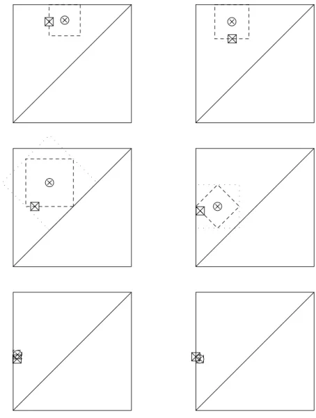
Figure 2 shows some steps of the simulation of our algorithm A (see also Algorithm 2 in Appendix A).
Figure 2: Illustration of the hitting-time simulation algorithm: The circled-cross gives the position of the particle at the beginning of the step. The squared-cross gives the position of the particles at the end of the step. The dashed square is the square given whose exit time and position is simulated, while the dotted square is the square first constructed, but intersecting some fissures and then rejected.
2.2
Exiting from a square
We remark that in the previous algorithm, we need to simulate random vari-ables giving us the first time τ(2) at which a stochastic process √2a−W
exits from a square when it starts at its center, together with the posi-tion√2a−Wτ(2), where W = (W(1), W(2)) is a standard 2d-Brownian Motion.
In fact, cWt/c2 is again a Standard Brownian Motion for any c > 0, and
the distribution of W is invariant under rotation. We may then assume that 2a− = 1 and that the square is [−1, 1]2. Hence, we are interested by the joint distribution of
τ(2) = inf{t > 0 | |Wt(i)| = 1 for i = 1 or i = 2} and Wτ(2).
2.2.1 Simulation of the exit time from the square
We have first to simulate the exit time from the square
C ={(x(1), x(2))∈ Rd| |x(i)| 6 1 for i = 1, 2}.
IfP2 is the distribution function of τ(2), then [MT99, Lemma 4.1, p. 741]
P2(t) =P[τ(2) < t] = 1− (1 − P(t))2 where
P(t) = P[τ(1) < t] with τ(1) = inf{t > 0 ∥ |W(1)
t | = 1}.
Hence, if U is a uniform random variable on [0, 1],P−1(1−√U ) is distributed
as τ(2).
The following formulas are borrowed from [MT99, Lemma 3.1, p. 737] and will be used to compute the distribution function P numerically:
P(t) = 1 − 4 π +∞ ∑ k=0 (−1)k 2k + 1exp ( −1 8π 2(2k + 1)2t ) , t > 0, (6a) P(t) = 2+∑∞ k=0 (−1)kerfc2k + 1√ 2t , t > 0 (6b) where erfc is the complementary of the error function:
erfc(x) = √2
π
∫ +∞
x
exp(−y2) dy. This distribution function P has density equal to
P′(t) = π 2 +∑∞ k=0 (−1)k(2k + 1) exp ( −1 8π 2(2k + 1)2t ) , t > 0, (7a) P′(t) = √2 2πt3 +∑∞ k=0 (−1)k(2k + 1) exp ( −1 2t(2k + 1) 2 ) , t > 0. (7b)
Formulae (6a) and (7a) are suitable for calculations under large t, when (6b) and (7b) are suitable under small t.
2.2.2 Exit position from the square
If one of the component of the 2-dimensional Brownian Motion is the first to hit a boundary of C at time τ , then the other remains in the interval [−1, 1] during [0, τ(2)]. Hence, to know Wτ(2), we compute the conditional probability
Q(β, t) = P[Wt< β| |Ws| < 1, 0 < s < t]. Using the computations in [MT99],
Q(β, t) = 1 1− P(t) 2 π +∑∞ k=0 1 2k + 1 ( (−1)k+ sinπ(2k + 1)β 2 ) × exp(−1 8π 2(2k + 1)2t ) , (8a) Q(β, t) = 1 1− P(t) ×+∑∞ k=0 (−1)k 2 erfc2k√− 1 2t − erfc 2k + β √ 2t − erfc2k + 2√ − β 2t + erfc 2k + 3 √ 2t . (8b)
As for P, (8a) is better for large t, when (8b) is suitable for small t. Of course, Q admits a smooth density, which is also expressible as series.
2.3
Simulation of exit time and position
We have now all the element to provide the algorithm to simulate (τ(2), W τ(2)),
when C is the square [−1, 1]2 [MT99, Theorem 4.1, p. 743].
We assume that ideally, the random variables generated by the function uniform are independent.
If C is the square with edges A1, A2, A3 and A4 whose edge length is 2d, then the time and position is given by the following algorithm:
Algorithm 1 Exit time and Position from a Square U ←uniform[0, 1] V ←uniform[0, 1] τ ← P−1(1−√U ) ξ ← Qτ−1(V ) (rem : ∈ [−1, 1]) k ←uniform{1, 2, 3, 4} return (2ad2 −τ, Ak+ ξ+1 2 −−−−−→ AkAk+1)
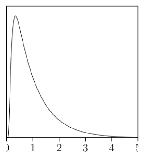
Figures 3 and 4 represent the distribution functionP and its density P′, while Figures 5 and 6 show the curve of the distribution function of Q(·, t) with its density Q′(·, t) for some values of t.
0 1 2 3 4 5
0 0.5 1
Figure 3: Distribution function P
0 1 2 3 4 5
0 0.5 1
Figure 4: DensityP′ of the distri-bution function P
t = 0.5 t = 0.1 t = 0.06 −1 −0.5 0 0.5 1 0 0.5 1
Figure 5: Distribution functionQ
t = 0.5 t = 0.1 t = 0.06 −1 −0.5 0 0.5 1 0 2 4
Figure 6: Density Q′ of the distri-bution function Q
3
Numerical results
L L periodic fissureFigure 7: Layered media
L L fissures
Figure 8: Sugar box
3.1
The layered media
The media is infinite in each direction, and is crossed by some horizontal fractures. The distance between a fracture and a fissure is equal to L (See Figure 7). The exchange coefficient is known in this simple case [QW96b], and is equal to
α = 12a− L2 .
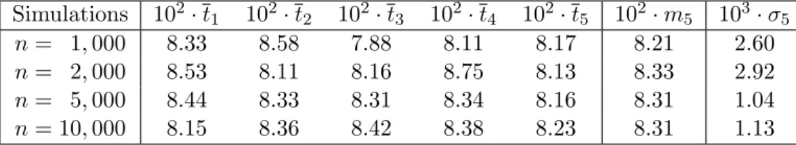
In the case of L is equal to 1 and a− = 1, the theoretical value ⟨t⟩ = 0.0833. The experiments in Table 1 shows that the methods provides some quite good results.
Simulations 102· t1 102· t2 102· t3 102· t4 102· t5 102· m5 103· σ5
n = 1, 000 8.33 8.58 7.88 8.11 8.17 8.21 2.60
n = 2, 000 8.53 8.11 8.16 8.75 8.13 8.33 2.92
n = 5, 000 8.44 8.33 8.31 8.34 8.16 8.31 1.04
n = 10, 000 8.15 8.36 8.42 8.38 8.23 8.31 1.13
Table 1: Mean of n experiments for the layered media with L = 1 and a− = 1. We set m5 = (t1+· · · + t5)/5 and σ5 = sd(t1, . . . , t5).
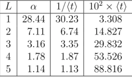
In Table 2, the dependence of L is studied. In fact, our algorithm is scale-independent, and the results behave as expected when L increases.
L α 1/⟨t⟩ 102× ⟨t⟩ 1 12.00 12.14 8.234 2 3.00 2.89 34.570 3 1.33 1.33 75.125 4 0.75 0.74 135.389 5 0.48 0.50 198.496
Table 2: Five experiments for 1, 000 simulations in the layered media in function of L
3.2
The sugar box
In this case, the media is composed of porous square box surrounded by some fractures. We have just to study the mean of the exit time for some particles launched with uniform distribution on a square of size L× L. The value of α computed by Warren and Root [WR63] is α = 28.44/L2. When L = 1, the theoretical value of the exit time is
⟨t⟩ = 0.0351.
Experiments in Table 3 show that this algorithm also provides some good results. Furthermore, the average number of steps is close to 4, as we might expect.
Simulations 102· t1 102· t2 102· t3 102· t4 102· t5 102· m5 103· σ5
n = 1, 000 3.36 3.51 3.63 3.45 3.48 3.49 1.00
n = 2, 000 3.39 3.61 3.35 3.54 3.45 3.47 1.08
n = 5, 000 3.53 3.59 3.52 3.53 3.51 3.54 0.29
n = 10, 000 3.49 3.56 3.56 3.41 3.49 3.50 0.63
Table 3: Mean of n experiments for the sugar box with L = 1 and a− = 1. We set m5 = (t1+· · · + t5)/5 and σ5 = sd(t1, . . . , t5).
Table 4 shows that the dependence in the size L of the sugar box is kept.
L α 1/⟨t⟩ 102× ⟨t⟩ 1 28.44 30.23 3.308 2 7.11 6.74 14.827 3 3.16 3.35 29.832 4 1.78 1.87 53.526 5 1.14 1.13 88.816
Table 4: Five experiments for 1, 000 simulations in the sugar box in function of L
3.3
Non trivial case
In this case, the fissures net is more complex: see Figure 9.
Figure 9: A non-trivial fissures net
In [CFL+00], the exchange coefficient is computed using a finite-volume method, and when L = 1 and a− = 1, its value is
We have to note that the model proposed in [CFL+00] is more complex than our, since the width of the fissure is not assume to be equal to 0, and the diffusion coefficient a+ in the fissure is not assumed to be infinite.
Using the random walk method proposed in [NE00, NEQ01, NEL01], the same authors have found a value
αr.w. = 34.18
for this geometry [NE98]. Here again, the width of the fissures is not ne-glected.
With 20,000 experiments with the conditions L = 1 and a− = 1, we found a value of
t = 0.028 and α = 1
t = 35.70. (9)
The average number of steps is 7.4, with a standard deviation of 6.9. Our value of α is close to the value of the exchange coefficients given by the other methods.
A
The algorithm in pseudo-language
The following functions are used in Algorithm 2:
Square(P, H): returns a square whose center is P and for which the the middle point of some edge is H.
Square diag(P, H): returns a square whose center is P and for which the point H is one of its corner.
ExitFromSquare(C): returns the exit time at which the Brownian particle at a given speed starting from the center of C goes out from the square C. It also returns the corresponding position.
References
[CFL+00] Y. Caillabet, P. Fabrie, P. Landereau, B. Nœtinger and M. Quintard. Implementation of a finite-volume method for the determination of effective parameters in fissured porous me-dia. Numer. Methods Partial Differential Equations, vol. 16, no2, pp. 237–263, 2000.
Algorithm 2 Simulation of the hitting time and position of the fissures
S1 particle (t, P ) in the matrix for (i∈ F ) do Hi ← orthogonal projection of P on (AiBi) δi ← d(P, [Ai, Bi]) end for j ← Arg min{δi; i∈ F } C ← square(P, Hj) if (a side of C ⊂ [Aj, Bj]) then exit_possible ← true for (i∈ F ; δi < √ 2δj) do if (C∩ [Ai, Bi]) then C ← square_diag(P, Hj) exit_possible ← false end if end for else if C ← square_diag(P, Hj) exit_possible ← false end if (τ, P′)← exit_from_square(C)
if [ (exit_possible) and (P′ ∈ [Aj, Bj]) ] then return (t + τ, P′)
else if
(t, P )← (t + τ, P′) goto S1
end if
[CLR00] F. Campillo, A. Lejay and E. Remy. A Monte-Carlo Method without Grid to Compute the Exchange Coefficient in the Double Porosity Model. Part II: In the Fissures. Preliminary Version, 2000.
[FOT94] M. Fukushima, Y. Oshima and M. Takeda. Dirichlet Forms
and Symmetric Markov Process. De Gruyter, 1994.
[GOO87] B. Gaveau, M. Okada and T. Okada. Second order differen-tial operators and Dirichlet integrals with singular coefficients. I: Functional calculus of one-dimensional operators. Tˆohoku Math. J.(2), vol. 39, no4, pp. 465–504, 1987.
[Lej00] A. Lejay. M´ethodes probabilistes pour l’homog´en´eisation des op´erateurs sous forme-divergence : cas lin´eaires et semi-lin´eaires.
PhD thesis, Universit´e de Provence, 2000. [url: www.iecn. u-nancy.fr/~lejay/].
[McC90] J.F. McCarthy. Effective permeability of sandstone–shale reser-voirs by random walk method. J. Phys. A: Math. Gen., vol. 23, pp. L445–L451, 1990.
[McC91] J.F. McCarthy. Analytical models of the effective permeability of sand–shale reservoirs. Geophys. J. Int., vol. 105, pp. 513–527, 1991.
[McC93a] J.F. McCarthy. Continuous–time random walks on random me-dia. J. Phys. A: Math. Gen., vol. 26, pp. 2495–2503, 1993. [McC93b] J.F. McCarthy. Reservoir characterization : Efficient random–
walk methods for upscaling and image selection. In Proceedings of
the SPE Asia Pacific Oil & Gas Conference & Exhibition. Singa-pore, 8–10 February, pp. 159–171, 1993.
[MD92] M. Mastrangelo and D. Dehen. Op´erateurs diff´erentiels paraboliques `a coefficients continus par morceaux et admettant un drift g´en´eralis´e. Bull. Sci. Math., vol. 116, pp. 67–93, 1992. 2`eme s´erie.
[MR91] Z. Ma and M. R¨ockner. Introduction to the Theory of
(Non-Symmetric) Dirichlet Forms. Universitext. Springer-Verlag, 1991.
[MT90] M. Mastrangelo and M. Talbi. Mouvement brownien
asym´etriques modifi´es en dimension finie et op´erateurs diff´erentiels `
a coefficients discontinus. Probability and Mathematical Statistics, vol. 11, pp. 47–78, 1990. Fasc. 1.
[MT99] G.N. Milstein and M.V. Tretyakov. Simulation of a space-time bounded diffusion. Ann. Appl. Probab., vol. 9, no3, pp. 732– 779, 1999.
[NE98] B. Nœtinger and T. Estebenet. Application of random walk methods on unstructured grids to up-scale fractured reservoirs. ECMOR VI Conf, Scotland, 1998.
[NE00] B. Nœtinger and T. Est´ebenet. Up-Scaling of Double Porosity Fractured Media Using Continuous-Time Random Walks Meth-ods. Transport in Porous Media, vol. 39, no3, pp. 315–337, 2000.
[NEL01] B. Nœtinger, T. Estebenet and P. Landereau. A direct determination of the transient exchange term of fractured media using a continuous time random walk method. Transport in Porous
Media, vol. 44, no3, pp. 539–557, 2001.
[NEQ01] B. Nœtinger, T. Estebenet and M. Quintard. Up-scaling flow in fractured media: equivalence between the large scale av-eraging theory and the continuous time random walk method.
Transport in Porous Media, vol. 43, no3, pp. 581–596, 2001. [Por79a] N.I. Portenko. Diffusion processes with a generalized drift
co-efficient. Theory Probab. Appl., vol. 24, no1, pp. 62–78, 1979. [Por79b] N.I. Portenko. Stochastic Differential Equations with
general-ized drift vector. Theory Probab. Appl., vol. 24, no2, pp. 338–353, 1979.
[QW96a] M. Quintard and S. Whitaker. Transport in chemically and mechanically heterogeous porous media. I: Theoritical develop-ment of region-averaged equations for sligthly compressible single-phase flow. Adv. Water Ressources, vol. 19, no1, pp. 29–47, 1996. [QW96b] M. Quintard and S. Whitaker. Transport in chemically and mechanically heterogeous porous media. II: Comparisons with nu-merical experiments for slightly compressible single-phase flow.
Adv. Water Ressources, vol. 19, pp. 49–60, 1996.
[Str88] D.W. Stroock. Diffusion Semigroups Corresponding to Uni-formly Elliptic Divergence Form Operator. In S´eminaire de Prob-abilit´es XXII, vol. 1321 of Lecture Notes in Math., pp. 316–347.
Springer-Verlag, 1988.
[WR63] J.E. Warren and P.J. Root. The Behavior of Naturally Frac-tured Reservoirs. Soc. Petrol. Eng. J., vol. 3, no3, pp. 245–255, 1963.