Model-based covariable decorrelation in linear regression (CorReg). Application to missing data and to steel industry

(1)

HAL Id: tel-01249789

https://hal.archives-ouvertes.fr/tel-01249789

Submitted on 4 Jan 2016

HAL is a multi-disciplinary open access archive for the deposit and dissemination of sci-entific research documents, whether they are pub-lished or not. The documents may come from teaching and research institutions in France or abroad, or from public or private research centers.

L’archive ouverte pluridisciplinaire HAL, est destinée au dépôt et à la diffusion de documents scientifiques de niveau recherche, publiés ou non, émanant des établissements d’enseignement et de recherche français ou étrangers, des laboratoires publics ou privés.

Model-based covariable decorrelation in linear regression

(CorReg). Application to missing data and to steel

industry

Clément Théry

To cite this version:

Clément Théry. Model-based covariable decorrelation in linear regression (CorReg). Application to missing data and to steel industry. Methodology [stat.ME]. Université Lille 1, 2015. English. �tel-01249789�

(2)

Université de Lille 1

ArcelorMittal

École doctorale ED Régionale SPI 72 Unité de recherche Laboratoire Paul Painlevé

Thèse présentée par Clément THÉRY

Soutenue publiquement le 8 juillet 2015

En vue de l’obtention du grade de docteur de l’Université de Lille 1

Discipline Mathématiques appliquées

Spécialité Statistique

Thèse dirigée par : ChristopheBIERNACKI

Composition du Jury

Rapporteurs Christian LAVERGNE Professeur à l’Université de Montpellier 3 François HUSSON Professeur à l’Agrocampus Ouest

Examinateur Cristian PREDA Professeur à l’Université de Lille 1

Invité Gaétan LORIDANT ArcelorMittal

Directeur de thèse Christophe BIERNACKI Professeur à l’Université de Lille 1 Titre de la thèse :

Model-based covariable decorrelation

in linear regression (CorReg).

(3)

(4)

Résumé

Les travaux effectués durant cette thèse ont pour but de pallier le problème des corréla-tions au sein des bases de données, particulièrement fréquentes dans le cadre industriel. Une modélisation explicite des corrélations par un système de sous-régressions entre co-variables permet de pointer les sources des corrélations et d’isoler certaines co-variables redondantes.

Il en découle une pré-sélection de variables nettement moins corrélées sans perte sig-nificative d’information et avec un fort potentiel explicatif (la pré-selection elle-même est expliquée par la structure de sous-régression qui est simple à comprendre car uniquement constituée de modèles linéaires).

Un algorithme de recherche de structure de sous-régressions est proposé, basé sur un modèle génératif complet sur les données et utilisant une chaîne MCMC (Monte-Carlo Markov Chain). Ce prétraitement est utilisé pour la régression linéaire comme une présélection des variables explicatives à des fins illustratives mais ne dépend pas de la variable réponse. Il peut donc être utilisé de manière générale pour toute problématique de corrélations.

Par la suite, un estimateur plug-in pour la régression linéaire est proposé pour ré-injecter l’information résiduelle contenue dans les variables redondantes de manière séquen-tielle. On utilise ainsi toutes les variables sans souffrir des corrélations entre covariables.

Enfin, le modèle génératif complet offre la perspective de pouvoir être utilisé pour gérer d’éventuelles valeurs manquantes dans les données. Cela permet la recherche de structure malgré l’absence de certaines données. Mais un autre débouché est l’imputation multiple des données manquantes, préalable à l’utilisation de méthodes classiques incompatibles avec la présence de valeurs manquantes. De plus, l’imputation multiple des valeurs man-quantes permet d’obtenir un estimateur de la variance des valeurs imputées. Encore une fois, la régression linéaire vient illustrer l’apport de la méthode qui reste cependant générique et pourrait être appliquée à d’autres contextes tels que le clustering.

Tout au long de ces travaux, l’accent est mis principalement sur l’interprétabilité des résultats en raison du caractère industriel de cette thèse.

Le package R intitulé CorReg, disponible sur le cran1 _{sous licence CeCILL}2_,

implé-mente les méthodes développées durant cette thèse.

Mots clés: Prétraitement, Régression, Corrélations, Valeurs manquantes, MCMC,

mod-èle génératif, Critère Bayésien, sélection de variable, méthode séquentielle, graphes.

1_{http://cran.r-project.org} 2_{http://www.cecill.info}

(5)

Abstract

This thesis was motivated by correlation issues in real datasets, in particular industrial datasets. The main idea stands in explicit modeling of the correlations between covariates by a structure of sub-regressions, that simply is a system of linear regressions between the covariates. It points out redundant covariates that can be deleted in a pre-selection step to improve matrix conditioning without significant loss of information and with strong explicative potential because this pre-selection is explained by the structure of sub-regressions, itself easy to interpret.

An algorithm to find the sub-regressions structure inherent to the dataset is provided, based on a full generative model and using Monte-Carlo Markov Chain (MCMC) method. This pre-treatment is then applied on linear regression to show its efficiency but does not depend on a response variable and thus can be used in a more general way with any correlated datasets.

In a second part, a plug-in estimator is defined to get back the redundant covariates sequentially. Then all the covariates are used but the sequential approach acts as a pro-tection against correlations.

Finally, the generative model defined here allows, as a perspective, to manage missing values both during the MCMC and then for imputation (for example multiple imputa-tion). Then we are able to use classical methods that are not compatible with missing datasets. Missing values can be imputed with a confidence interval to show estimation accuracy. Once again, linear regression is used to illustrate the benefits of this method but it remains a pre-treatment that can be used in other contexts, like clustering and so on. The industrial motivation of this work defines interpretation as a stronghold at each step.

The R package CorReg, is on cran3 _{now under CeCILL}4 _{license. It implements the}

methods created during this thesis.

Keywords: Pre-treatment, Regression, Correlations, Missing values, MCMC,

genera-tive model, Bayesian Criterion, variable selection, plug-in method,. . .

3_{http://cran.r-project.org} 4_{http://www.cecill.info}

(6)

Acknowledgements

I want to thank ArcelorMittal for the funding of this thesis, the opportunity to make this thesis with real datasets and the confidence in this work that has led me to be recruited since May.

But this work would not have been possible without the help of Gaétan LORIDANT, my hierarchic superior and friend who has convinced ArcelorMittal to fund this thesis and helped me in this work by a strong moral support and spending a great amount of time with me to find the good direction between academic and industrial needs with some technical help when he could. I would not have made all this work without him.

I also want to thank Christophe BIERNACKI, my academic director who accepted to lead this work even if the subject was not coming from the university. He also has spent a lot of time on this thesis with patience and has trust in the new method enough to share it with others, and it really means a lot to me.

The last year I have worked mostly in the INRIA center with M dal team, especially those from the "bureau 106 " who helped me to put CorReg on cran (in particular Quentin GRIMONPREZ) and those who had already submitted something on cran know that it is not always fun to achieve this goal. They also helped me in this last and tough year just by their presence, giving me the courage to go further.

I finally want to thank my family. My wife who had to support most of the charge of the family on top of her work and to let me work during the holidays, and my three sons, Nathan, Louis and Thibault who have been kind with her even if they rarely saw their father during the week. I love them and am thankful for their comprehension.

(7)

I Model for regression with correlation-free covariates

42

4 Structure of inter-covariates regressions 43 4.1 Introduction . . . 43

4.2 Explicit modeling of the correlations . . . 44

4.3 A by-product model: marginal regression with decorrelated covariates . . . 45

4.4 Strategy of use: pre-treatment before classical estimation/selection methods 46 4.5 Illustration of the trade-off conveyed by the pre-treatment . . . 47

4.6 Connexion with graphs . . . 48

4.7 mse comparison on the running example . . . 50

4.8 Numerical results with a known structure on more complex datasets . . . . 57

4.8.1 The datasets . . . 57

4.8.2 Results when the response depends on all the covariates, true struc-ture known . . . 57

5 Estimation of the structure of sub-regression 65 5.1 Model choice: Brief state of the art . . . 65

5.1.1 Cross validation . . . 65

5.1.2 Bayesian Information Criterion (bic) . . . 66

5.2 Revisiting the Bayesian approach for an over-penalized bic . . . 66

5.2.1 Probability associated to the redundant covariates (responses) . . . 66

5.2.2 Probability associated to the free covariates (predictors) . . . 67

5.2.3 Probability associated to the discrete structure S . . . 67

5.2.4 Penalization of the integrated likelihood by P(S) . . . 68

5.3 Random walk to optimize the new criterion . . . 69

5.3.1 Transition probabilities . . . 69

5.3.2 Deterministic neighbourhood . . . 69

5.3.3 Stochastic neighbourhood . . . 70

5.3.4 Enlarged neighbourhood by constraint relaxation . . . 71

5.3.5 Pruning . . . 74

5.3.6 Initialization of the walk . . . 74

5.3.7 Implementing and visualizing the walk by the CorReg software . . . 77

6 Numerical results on simulated datasets 79 6.1 Simulated datasets . . . 79

6.2 Results about the estimation of the structure of sub-regression . . . 79

6.2.1 Comparison with Selvarclust . . . 80

6.2.2 Computational time . . . 82

6.3 Results on the main regression with specific designs . . . 84

6.3.1 Response variable depends on all the covariates . . . 84

6.3.2 Response variable depends only on free covariates (predictors) . . . 90

6.3.3 Response variable depends only on redundant covariates . . . 96

6.3.4 Robustness with non-linear case . . . 102

(9)

7 Experiments on steel industry 103

7.1 Quality case study . . . 103

7.2 Production case study . . . 105

II Two extensions: Re-injection of correlated covariates and

Dealing with missing data

108

8 Re-injection of correlated covariates to improve prediction 109 8.1 Motivations . . . 109

8.2 A plug-in model to reduce the noise . . . 110

8.3 Model selection consistency of lasso improved . . . 114

8.4 Numerical results with specific designs . . . 115

8.4.1 Response variable depends on all the covariates . . . 115

8.4.2 Response variable depends only on free covariates (predictors) . . . 121

8.4.3 Response variable depends only on redundant covariates . . . 121

9 Using the full generative model to manage missing data 133 9.1 State of the art on missing data . . . 133

9.2 Choice of the model of sub-regressions despite missing values . . . 134

9.2.1 Marginal (observed) likelihood . . . 134

9.2.2 Weighted penalty for bicú . . . 136

9.3 Maximum likelihood estimation of the coefficients of sub-regression . . . . 137

9.3.1 Stochastic EM . . . 137

9.3.2 Stochastic imputation by Gibbs sampling . . . 139

9.3.3 Parameters computation for the Gibbs sampler . . . 140

9.4 Missing values in the main regression . . . 142

9.5 Numerical results on simulated datasets . . . 142

9.5.1 Estimation of the sub-regression coefficients . . . 142

9.5.2 Multiple imputation . . . 143

9.5.3 Results on the main regression . . . 144

9.6 Numerical results on real datasets . . . 145

10 Conclusion and prospects 147 10.1 Conclusion . . . 147

10.2 Prospects . . . 148

10.2.1 Qualitative variables . . . 148

10.2.2 Regression mixture models . . . 148

10.2.3 Using the response variable to estimate the structure of sub-regression148 10.2.4 Pre-treatment for non-linear regression . . . 149

10.2.5 Missing values in classical methods . . . 149

10.2.6 Improved programming and interpretation . . . 150

References 151

(10)

A Identifiability 159

A.1 Definition . . . 159 A.2 Sufficient condition for identifiability . . . 159

(11)

Glossary of notations

This glossary can be used to find the meaning of some notations without having to search within the chapters. Bold characters are used to distinguish multidimensional objects. Many objects are tuples.

• –j is the vector of the coefficients of the jth sub-regression. • – = (–1, . . . , –dr) is the dr≠uple of the –j.

• –ú is the d

f ◊ dr matrix of the sub-regressions coefficients.

• ¯– is the d ◊ d matrix of the sub-regression coefficients with ¯–i,j the coefficients associated to Xi _{in the sub-regression explaining X}j_.

• —f = —Jf is the (d ≠ dr) ◊ 1 vector of the regression coefficients associated to the free covariates in the main regression on Y .

• —r= —Jr is the dr◊1 vector of the regression coefficients associated to the responses covariates.

• d is the number of covariates in the dataset X. • df is the number of free covariates in the dataset.

• dp = (d1p, . . . , ddpr) the dr-vector of the number of predictors in the sub-regressions. • dr is the number of response covariates in the dataset (and consequently the number

of sub-regressions).

• Á is the n ◊ dr matrix of the Áj.

• Jf = {1, . . . , d}\Jr is the set of all non response covariates.

• Jp = (Jp1, . . . , Jpdr) the dr-uple of all the predictors for all the sub-regressions. • Jj

p is the vector of the predictors for the jth sub-regression. • Jr the set of the indices of the dr response variables. • Jr = (Jr1, . . . , Jrdr) the dr-uple of all the response variables. • Jj

r is the index of the jth response variable.

• K is the number of components of the Gaussian mixture followed by X. • Kj is the number of components of the Gaussian mixture followed by Xj.

• µX is the d≠uple of the K ◊ 1 vectors µXj of the means associated to Xj in X. • µXj is the K ◊ 1 vector of the means associated to Xj in X.

(12)

• µj is the Kj ◊ 1 vector of the means of the Gaussian mixture followed by Xj with

j œ Jf.

• µi,Jrj is the Ki,Jrj≠uple of the means of the Gaussian mixture followed by the condi-tional distribution of x_i,Jj

r knowing its observed regressors X Jpj i,O. • µj,k is the kth element of µj.

• µi,Jrj,k is the mean of the k

th component of the Gaussian mixture followed by the conditional distribution of x_i,Jj

r knowing its observed regressors X Jpj i,O.

• fiX is the K ◊ 1 vector of proportions of the Gaussian mixture followed by X. • fij is the Kj ◊ 1 vector of proportions of the Gaussian mixture followed by Xj. • fik is the proportion of the kth component of the Gaussian mixture followed by X. • fii,Jrj is the Ki,Jrj≠uple of the proportions of the Gaussian mixture followed by the

conditional distribution of x_i,Jj

r knowing its observed regressors X Jpj i,O.

• ﬁj,k is the proportion of the kth component of the Gaussian mixture followed by Xj. • ﬁi,Jrj,k is the proportion of the k

th component of the Gaussian mixture followed by the conditional distribution of x_i,Jj

r knowing its observed regressors X Jpj i,O. • ‡j2 is the variance of the residual of the jth sub-regression.

• X is the d≠uple of the K ◊ 1 vectors Xl of the variances associated to Xl in the Gaussian mixture followed by X.

• Xl is the K ◊ 1 vector of the variances associated to Xl in the Gaussian mixture followed by X.

• i,Jrj is the Ki,Jrj≠uple of the variances of the Gaussian mixture followed by the conditional distribution of x_i,Jj

r knowing its observed regressors X Jpj i,O. • Xl_,k is the variance of Xl in the kth component of X.

• i,Jrj,k is the variance of the k

th component of the Gaussian mixture followed by the conditional distribution of x_i,Jj

r knowing its observed regressors X Jpj i,O. • is the set of the parameters associated to the Gaussian mixtures on Xf.

• X is the n ◊ d matrix whose columns are the covariates in the datasets and rows are the individuals.

• Xj is the jth column of X.

• Xr is the matrix of the response covariates. • Xf is the matrix of the predictor covariates.

• XO= (X1,O, . . . , Xn,O) is the n≠uple of the Xi,O. • Xij¯ = (xi,1, . . . , xi,j≠1, xi,j+1, . . . , xi,d).

(13)

• Xi,O is the vector of the observed values for the ith individual of X. • XJf

i,O is the vector of the observed values for the ith individual of Xf. • XJr

i,O is the vector of the observed values for the ith individual of Xr. • Y is the n ◊ 1 response variable in the main regression.

(14)

Chapter 1 Introduction

Abstract: This chapter describes the industrial constraints and the mathematical

con-text that have led to this work. This work takes place in a steel industry concon-text and was funded by ArcelorMittal, the world leading company in steel making.

1.1 Industrial motivation

1.1.1 Steel making process

Steel making starts from raw materials and aims to give highly specific products used in automotive, beverage cans, etc. We first melt down a mix of iron ore and cock to obtain cast iron that is then transformed in steel by addition of pure oxygen to remove carbon. Liquid steel is then refreshed in a mould (continuous casting) to obtain steel slabs (nearly 20 tons each, 23 cm thick).

Cold slabs are then warmed to be pressed in a hot rolling mill to obtain coils (nearly half a millimetre thick or less). This warming phase also allows to adjust mechanical properties of the final product. It is the process that gave its name to the simulated an-nealing algorithm that allows to escape from local extrema thanks to a parameter called "temperature" in allusion to the steel making process.

If the final product requires a thinner strip of steel, coils pass through a cold rolling mill. Figure 1.1 provides some illustrations of the steel making process. Each step of this process involves a whole manufacture and the whole process can take several weeks. The most sensitive products are the thinner ones and sometimes defects are generated by small inclusions in the steel down to the dozen of microns. So even if quality is evaluated at each step of the process, some defects are only found when the whole process is finished even if the origin comes from the first part of this process. So we have hundreds of parameters to analyse.

Steel making is continuously improving and we are now able to produce steel that is both thinner and stronger. Steel is 100% recyclable unlike petroleum so we will continue to use it widely in the future. This quickly evolving industry is associated to a lot of research in metallurgy but also needs adapted statistical tools. That is why this thesis has been made.

(15)

Figure 1.1: Quick overview of the steel making process, from hot liquid metal to coils.

1.1.2 Impact of the industrial context

The main objective is to be able to solve quality crisis when they occur. In such a case, a new type of unknown quality issue is observed and we may have no idea of its origin. Defects, even generated at the beginning of the process, are often detected in its last part. The steel-making process includes several sub-process. Thus we have many covariates and no a priori on the relevant ones. Moreover, the values of each covariate are linked to the characteristics of the final product, and many physical laws and tuning models are implied in the process. Therefore the covariates are highly correlated. We have several constraints:

• Being able to predict the defect and stop the process as early as possible to gain time (and money)

• Being able to find parameters that can be changed and to understand the origin of the defect because the objective is not only to understand but to adapt the problematic part of the process.

• It also must be fast and automatic (without any a priori) to manage totally new phenomenon on new products.

We will see in the state of the art that correlations are a real issue and that the number of variables increases the problem. The stakes are very high because of the high productivity of the steel plants and the extreme competition between steel makers but also because steel making is now well-known and optimized thus new defects only appears on innovative steels with high added value. Any improvement on such crisis can have important impact on market shares and when the customer is impacted, each day won by the automation of the data mining process can lead to substantial savings. So we really need a kind of automatic method, able to manage correlations without any a priori and giving an easily understandable and flexible model.

(16)

1.1.3 Industrial tools

Our goal was also to demonstrate that statistics can provide efficient methods for real datasets, easy to use and understand. This was a battle against correlations but also against scepticism.

Figure 1.2 shows the kind of results proposed by a rule-based software that is sold as a non-statistical tool. It is just a partition of the sample by binary rules (like regres-sion trees in Section 3.1.3). Some blur is added to the plot to help interpretation. The algorithm used here is somewhere between exhaustive research and decision trees. It is extremely slow (research with d > 10 would take years) and is less efficient than regression trees. Morever, it requires to discretize the response variable to obtain “good” and “bad” values. The green rectangle is very far from the true green zone even for this toy example provided by the reseller.

Ergonomy and quality of interpretation are stakes for us to make engineers use efficient methods instead of this kind of stuff.

(a) Without blur (b) With some blur proportional to the density of points

Figure 1.2: Result on a toy example provided by FlashProcess, similar to decision trees but less efficient and extremely slower. Colors are part of the learning set.

1.2 Mathematical motivation

Every engineer, even non-statistician uses frequently linear regression to seek relation-ship between some covariates. It is easy to understand, fast to do, and is used in nearly all the fields where statistics are involved [Montgomery et al., 2012]: Astronomy [Isobe et al., 1990], Sociology [Longford, 2012], and so on. It can be done directly in Mi-crosoft Excel which is well known and often used by engineers to open and analyse most of their datasets. Thus we have chosen to work in this way.

Popularity of regression can be confirmed by the fact that, as of 2014, Google Scholar proposes more than 3.8 millions of papers related to regression and many of them were cited several thousands times (in other papers). Linear regression is an old strategy well known and with many derivatives (as we will see in the following) and can be ex-tended to more general and complex problems using a link function between the response

(17)

Figure 1.3: An example of simple linear regression

variable and the linear model (Generalized Linear Model, see [Kiebel and Holmes, 2003, Wickens, 2004, Nelder and Baker, 1972] and also [McCullagh and Nelder, 1989]). Its sim-plicity facilitates a wide spread usage in industry and other fields of application. It is also a good tool for interpretation with the sign of the coefficients indicating whether the as-sociated covariate has a positive or negative impact on the response variable.

More complex situations can be described by evolved forms of linear regression like the hierarchical linear model [Raudenbush, 2002, Woltman et al., 2012] or multilevel re-gression [Moerbeek et al., 2003, Maas and Hox, 2004, Hox, 1998] that allows to consider effects of the covariates on nested sub-populations in the dataset. It is like using interac-tions but with a proper modeling that improves interpretation. It is not really a linear model because it is not linear in the original covariates but can be seen as a basis ex-pansion using new covariates (the interactions) composed of the product of some of the original covariates.

But linear regression is in trouble when correlations between the covariates are strong, as we will see later (Chapter 3). So we have decided to investigate some ways to over-come correlations issues in linear regression, keeping in mind industrial constraints about variable selection and interpretability.

1.3 Outline of the manuscript

After a substantial abstract in french (Chapter 2), we start with a brief state of the art (Chapter 3) that lists some classical regression methods and explains that they do not respect our industrial needs because of correlation issues or lack of variable selection or interpretability. It leads us to define a new model.

In the first part, we define an explicit structure of sub-regressions (Chapter 4) to ex-plain correlations between the covariates. Then we use this structure to obtain a reduced model (by marginalization) with uncorrelated covariates. It can be seen as a kind of vari-able pre-selection that allows further usage of any estimator (including varivari-able selection tools). The structure itself is used for interpretation by the distinction between redun-dant and irrelevant covariates. An MCMC algorithm is provided (Chapter 5) to find the sub-regressions structure, relying on a Bayesian criterion and a full generative model on the covariates. Numerical results are then provided on both simulated datasets (Chapter

(18)

6) and real datasets (Chapter 7) from steel industry without too much details because of industrial secret. The package CorReg, on CRAN, implements all this work and allows to retrieve the results given here.

In a second part, we use the marginal model and its estimated residuals to obtain a new sequential model by plug-in (Chapter 8) that is asymptotically unbiased (the marginal one could be biased). Another application of the generative model on the dataset and the structure of sub-regressions is that we are able to compute conditional distributions and then to manage missing values (Chapter 9).

Conclusion: Industrial context necessitates easily understandable models and the stakes

are frequently very high in terms of financial impact. These two points give strong con-straints because used methods has to be accessible for non-statisticians in a minimum amount of time and results obtained have to be clearly interpretable (no black-box). So a powerful tool without interpretation becomes kind of useless in such a context.

Then we need a tool that is both easy to use and to understand, giving priority to inter-pretation more than prediction. The tool will have to work without a priori and to be able to select relevant covariates.

(19)

Chapter 2 Résumé substantiel en français

2.1 Position du problème

La régression linéaire est l’outil de modélisation le plus classique et se résume à une équation bien connue

Y = X— + ÁY

où Y est la variable réponse de taille n◊1 que l’on souhaite décrire à l’aide de d variables explicatives1 _{observées sur n individus et dont les valeurs sont stockées dans la matrice}

X de taille n ◊ d. Le vecteur — est le vecteur des coefficients de régression qui permet de

décrire le lien linéaire entre Y et X. Le vecteur ÁY est un bruit blanc gaussien N (0, ‡2YIn) qui représente l’inexactitude du modèle de régression.

On connaît l’estimateur sans biais de variance minimale (ESBVM) de — qui est obtenu par Moindres Carrés Ordinaires (MCO) selon la formule :

ˆ— = (XÕ_X₎≠1_XÕ_{Y .}

Le calcul de cet estimateur nécessite l’inversion de la matrice (XÕ_X_{) qui est mal}

condi-tionnée si les variables explicatives sont corrélées entre elles. Ce mauvais conditionnement nuit à la qualité de l’estimation et vient impacter la variance de l’estimateur comme le montre la formule :

VarX(ˆ—) = ‡2Y(XÕX)≠1

C’est cette situation problèmatique que nous nous proposons d’améliorer.

2.2 Modélisation explicite des corrélations

Le mauvais conditionnement de la matrice provient de la quasi-singularité (parfois singu-larité numérique) de celle-ci quand les colonnes de X sont presque linéairement dépen-dantes. Cette quasi dépendance linéaire peut être elle aussi modélisée par régression lineaire. On se propose donc de considérer notre problématique comme l’existence d’un modèle de sous-régressions au sein des variables explicatives avec certaines des variables expliquées par d’autres, formant ainsi une partition des d variables en 2 blocs : les variables réponses (expliquées) et les variables prédictives. Notre modèle repose sur 2 hypothèses fondamentales :

1_{En général on ajoute une constante parmi les régresseurs. Par exemple X}1_{= (1, . . . , 1)}Õ_{. Le coefficient}

(20)

Hypothèse 1 Les corrélations entre covariables viennent uniquement de ce que certaines

d’entre elles dépendent linéairement d’autres covariables. Plus précisément, il y a dr Ø 0

“sous-regressions”, chaque sous-regression j = 1, . . . , dr ayant la variable XJ j

r comme

variable réponse (Jj

r œ {1, . . . , d} et Jrj ”= Jj

Õ

r pour j ”= jÕ) et ayant les djp > 0 variables

XJpj comme variables predictives (Jj

p µ {1, . . . , d}\Jrj et djp = |Jpj| le cardinal de Jpj) : XJrj = XJpj_– j+ Áj, (2.1) où –j œ Rd j r (–h j ”= 0 pour tout j = 1, . . . , dr et h = 1, . . . , djp) et Áj ≥ Nn(0, ‡2jI).

Hypothèse 2 Nous supposons également que les variables réponses et les variables

pré-dictives forment deux blocs disjoints dans X : pour toute sous-régression j = 1, . . . , dr,

Jj

p µ Jf où Jr = {Jr1, . . . , Jrdr} est l’ensemble de toutes les variables réponses avec

Jf = {1, . . . , d}\Jr l’ensemble des variables non expliquées de cardinal df = d ≠ dr = |Jf|.

Cette seconde hypothèse garantit l’obtention d’un système de sous-régression très simple et sans imbrications ni surtout aucun cycle. Cette hypothèse n’est pas trop restrictive dans la mesure où tout système sans cycle peut (par substitutions) être reformulé sous cette forme simplifiée (avec une variance accrue).

Notations Par la suite nous noterons Jr = (Jr1, . . . , Jrdr) le dr-uplet des variables réponses (à ne pas confondre avec Jr défini plus haut), Jp = (Jp1, . . . , Jpdr) le dr-uplet des prédicteurs de toutes les sous-régressions, dp = (d1p, . . . , ddpr) les nombres correspon-dants de predicteurs et S = (Jr, Jp) le model global (structure de sous-régressions). Pour alléger les notations, on définit alors Xr = XJr la matrice des variables réponses et

Xf = XJf la matrice de toutes les autres variables, ainsi considérées comme libres (free en anglais). Les valeurs des paramètres sont également concaténées : – = (–1, . . . , –dr) est le dr≠uplet des vecteurs des coefficients de sous-régression et ‡2 = (‡12, . . . , ‡d2r) le vecteur des variances associées :

Xr = Xf–ú+ Á (regression multiple multivariée)

où la matrice Á œ Rn◊dr est la matrice des bruits des sous-régressions composée des colonnes Áj ≥ N (0, ‡j2In) que nous supposons indépendantes entre elles et –ú œ Rdf◊dr est la matrice des coefficients des sous-régressions avec (–ú

j)Jpj = –j et (–

ú

j)Jf\Jpj = 0. Ces notations sont illustrées dans l’exemple ci-après.

Données d’exemple : d = 5 variables dont 4 gaussiennes centrées réduites i.i.d.

Xf = (X1, X2, X4, X5) et une variable redondante Xr = X3 = X1 + X2 + Á1 avec

Á1 ≥ N (0, ‡12In). Deux régressions principales en Y sont testées avec — = (1, 1, 1, 1, 1)Õ et ‡Y œ {10, 20}. Le conditionnement de (XÕX) se déteriore donc quand ‡1 diminue. Ici

Jf = {1, 2, 4, 5}, Jr = {3}, Jr = (3), dp = 2, Jp = ({1, 2}), – = (–1) = ((1, 1)Õ), XJ

1

p = (X1_{, X}2_{), S = ((3), ({1, 2})). On note R}2 _{est le coefficient de détermination :}

R2 = 1 ≠ Var(Á1)

Var(X3₎ (2.2)

La figure 3.5 page 29 illustre la détérioration de l’estimation quand les sous-régressions deviennent trop fortes (R2 _{proche de 1) pour différentes valeurs de n sur nos données}

(21)

Remarques

• Les sous-régressions définies en (2.1) sont très simples à comprendre pour l’utilisateur et permettent donc d’avoir un aperçu net des corrélations présentes dans les données étudiées.

• S ne dépend pas de Y et peut donc être estimé séparément.

2.3 Modèle marginal

Le fait de modéliser explicitement les corrélations entre les covariables nous permet de réécrire le modèle de régression principal. On peut en effet substituer les variables redon-dantes par leur sous-régression, ce qui revient à intégrer la régression sur Xr sachant la structure de sous-régressions S. On fait alors une hypothèse supplémentaire :

Hypothèse 3 On suppose l’indépendance 2 à 2 entre les erreurs de régression ÁY et

les Áj, avec j œ {1, . . . , dr}. En particulier on a l’indépendance conditionnelle entre les

variables réponses : {XJrj_|XJpj_{, S}; –

j, ‡j2} définies par l’équation (2.1). On a donc P(Xr|Xf, S; –, ‡2) = dr Ÿ j=1 P(XJrj_|XJpj_{, S}; – j, ‡j2) P(Y |Xf, S; —, –, ‡2Y, ‡2) = ⁄ RdrP(Y |Xr, Xf, S; —, ‡ 2 Y)P(Xr|Xf, S; –, ‡2)dXr, ce qui donne Y = Xf—f + Xr—r+ ÁY Y = Xf(—f + dr ÿ j=1 —_Jj r– ú j) + dr ÿ j=1 —_Jj rÁj + ÁY (2.3) = Xf—úf + ÁúY où —r = —Jr, —f = —Jf.

On se retrouve donc avec un modèle marginal plus parsimonieux, sans biais sur Y (vrai modèle) mais avec une variance potentiellement accrue. Cet accroissement de la variance est proportionnel à Á qui est la matrice des résidus des sous-régressions. Plus les sous-régressions sont fortes et plus cette variance est faible. Tout le principe du modèle marginal repose sur le compromis entre l’amélioration du conditionnement de (XÕ_X_{) par suppression des variables redondantes et aussi la réduction de la dimension}

(le modèle marginal ne nécessite que l’inversion de (XÕ

fXf)) face au léger accroissement de la variance issu de la marginalisation. On va donc comparer

ˆ— = (XÕ_X₎≠1_XÕ_Y _{au modèle marginal}

ˆ—ú

f = (XÕfXf)≠1XÕfY

Les deux modèles sont de dimension différente, on compare donc leurs erreurs moyennes quadratiques respectives (mse en anglais pour Mean Squared Error):

mse(ˆ—|X) = ‡2 Y Tr(XÕX)≠1 mse(ˆ—ú|X) = Î dr ÿ j=1 —_Jj r– ú j Î22 + Î —rÎ22 +(‡Y2 + dr ÿ j=1 ‡_j2—_J2j r) Tr(X Õ fXf)≠1

(22)

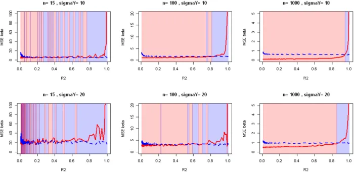
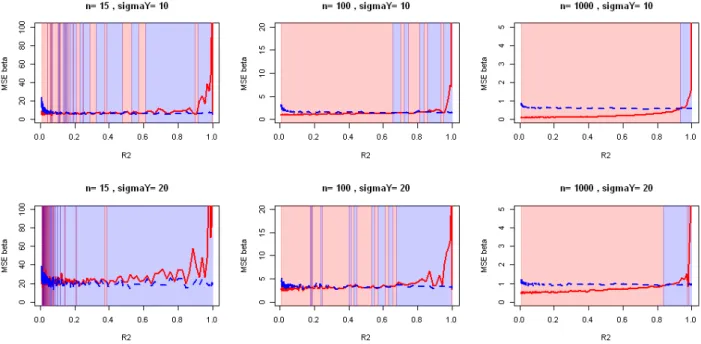
Ces deux équations illustrent bien le compromis biais-variance du modèle marginal. La figure 4.2 page 51 compare les erreurs d’estimation obtenues pour différentes valeurs des paramètres, montrant la nette amélioration rendue possible par la marginalisation. Quand

n tend vers l’infini les traces tendent vers 0 et donc le modèle complet devient meilleur

(car sans biais). Mais pour n fixé, quand les ‡2

j tendent vers 0 la trace dans le MSE du modèle complet explose (les sous-régressions tendent à devenir exactes) et la variance du modèle marginal diminue donc l’explosion du mse du modèle complet finit par dépasser le biais du modèle marginal et le mse du modèle marginal devient le plus faible. On remarque enfin que quand —r est nul, le modèle marginal est le vrai modèle et devient donc meilleur que le modèle complet (qui estime en vain —r, même s’il est sans biais).

Remarque Les hypothèses 1 à 3, impliquent que les variables dans Xf ne sont pas

corrélées (covariance nulle : voir Lemme en section A.2).

2.4 Notion de prétraitement

Le modèle marginal peut être vu comme un pari: on décide (pour s’affranchir des prob-lèmes liés aux corrélations) de ne retenir que Xf pour la prédiction. Il s’agit d’un prétraitement par sélection de variables puisqu’on se ramène à un modèle de régres-sion linéaire classique pour lequel n’importe quel estimateur peut être utilisé. Cela fait de ce modèle un outil générique. La préselection permet de cibler des variables qui n’interviendront pas dans le modèle final sans pour autant être indépendantes de Y . Le modèle final est donc parsimonieux mais ne fausse pas l’interprétation. L’estimation de —ú _{peut ensuite se faire en utilisant une quelconque méthode de sélection de variables}

pour éliminer les variables qui, elles, ne sont pas pertinentes pour expliquer Y .

On obtient donc deux types de 0 : ceux de la marginalisation qui pointent les vari-ables redondantes et ceux de sélection qui viennent dans un second temps et pointent les variables indépendantes. L’interprétation est donc enrichie par rapport à une méthode de sélection classique qui fournirait le même modèle final. Or, le contexte industriel de ces travaux rend indispensable d’avoir une bonne qualité d’interprétation. L’objectif est donc atteint pour ce point précis. Notre modèle marginal est un outil de décorrélation de variables par préselection.

2.5 Estimation de la structure

La raison d’être de notre modèle marginal est la fragilité des méthodes de régression face à des covariables fortement corrélées. Il serait donc vain d’essayer les sous-régression en estimant les modèles de régression de chaque variable en fonction de toutes les autres car les corrélations nuisent à l’efficacité de ces modèles. Pour cette raison, nous avons établi un algorithme MCMC pour trouver le meilleur modèle de sous-régressions. L’idée consiste à voir la structure de sous-régression comme un paramètre binaire, une matrice binaire creuse pour être plus précis. Cette matrice G de taille d ◊ d correspond à une matrice d’adjacence qui indique les liaisons entre covariables de la manière suivante : Gi,j = 1 si, et seulement si Xj _{est expliqué par X}i_.

Chaque étape (q + 1) de l’algorithme propose de garder la structure G(q) _{en cours ou}

bien de bouger vers une structure candidate qui diffère de G(q)_{en un unique point. Ainsi,}

selon les cas, les candidats vont allonger ou réduire des sous-régressions, les supprimer ou les créer.

(23)

Pour pouvoir trancher entre plusieurs candidats, nous avons besoin d’une fonction coût qui soit capable de comparer des modèles avec des nombres distincts de sous-régressions. Nous définissons alors un modèle génératif complet sur X qui complète le modèle de sous-régressions en établissant des modèles de mélanges gaussiens indépendants pour les variables de Xf. Une fois ce modèle génératif établi, nous pouvons utiliser le critère bic pour comparer les différents modèles et conduire chaque étape de la chaîne MCMC par un tirage aléatoire pondéré par les écarts entre les bic des différents modèles proposés (dont le modèle en cours). L’algorithme continue ainsi sa marche et fournit à l’utilisateur le modèle rencontré (qu’il ait été choisi ou non) qui a le meilleur bic.

La chaîne MCMC est conditionnée par le critère de partitionnement : les variables expliquées ne doivent en expliquer aucune autre (hypothèse 2). Chaque modèle réal-isable peut être entièrement construit ou déconstruit pendant la marche aléatoire donc l’algorithme suit une chaîne de Markov régulière [Grinstead and Snell, 1997]. Ainsi il est certain que, asymptotiquement (en nombre d’étapes), l’algorithme trouve le modèle ayant le meilleur bic.

2.6 Relaxation des contraintes et nouveau critère

Pour améliorer la mélangeance de l’algorithme et donc sa vitesse de convergence, on peut jouer avec la contrainte de partitionnement par une méthode de relaxation semblable à un recuit simulé. Quand une structure candidate n’est pas réalisable (ne produit pas de partition), on peut la modifier en d’autres endroits pour la rendre réalisable. Il suffit de suivre les formules suivantes pour une modification en (i, j) de la matrice G :

1. Modification (suppression/création) de l’arc (i, j) :

G(q+1)i,j = 1 ≠ G

(q)

i,j

2. Si la variable Xi _{devient un prédicteur elle ne peut plus être une variable réponse :}

G(q+1)_.,i = G(q)_i,jG(q)_.,i

3. Si la variable Xj devient une variable réponse elle ne peut plus être un prédicteur :

G(q+1)_j,. = G(q)_i,jG(q)_j,.

où G(q+1)i,j est la valeur de la matrice G(q+1) ligne i et colonne j, G

(q+1)

.,i est la iième colonne de G(q+1) _{et G}(q+1)

j,. la jième ligne de G(q+1). Cette méthode de relaxation permet de sortir rapidement des extrema locaux et améliore donc significativement l’efficacité de l’algorithme (Figure 5.10 page 77). La méthode est illustrée sur un exemple par les fig-ures 5.1 à 5.6 (pages 72 à 73).

Mais il reste un problème. Le nombre de modèles envisageables est considérable et le critère bic ne tient pas compte de cette quantité, menant à des modèles trop complexes. On lui ajoute donc une pénalité qui tient compte du nombre de modèles réalisables pour pénaliser plus lourdement les modèles complexes. De manière générale quand on estime la vraisemblance d’une structure S dans une base de données X, bic est utilisé comme approximation pour P(S|X) Ã P(X|S)P(S) car P(S) est consid-éré comme suivant une loi uniforme. Ici on s’appuie sur une loi uniforme hiérarchique

(24)

PH(S) = PU(Jp|dp, Jr, dr)PU(dp|Jr, dr)PU(Jr|dr)PU(dr) pour ajouter une pénalité sup-plémentaire aux structures complexes (même probabilité globale pour un plus grand nombre de structures donc chaque structure devient moins probable). On note bicH ce nouveau critère. Ce critère pénalise plus lourdement les modèles ayant de nombreux paramètres mais conserve les propriétés asymptotiques de bic.

Ces deux outils viennent améliorer l’efficacité de l’algorithme sans paramètre utilisa-teur à optimiser par ailleurs. Tout reste naturel et intuitif pour une meilleure automati-sation.

2.7 Résultats

La méthode a été testée sur données simulées puis réelles, montrant l’efficacité du modèle marginal s’appuyant sur la vraie structure de sous-régressions (section 4.7), l’efficacité de l’algorithme de recherche de structure (section 6.2), et l’efficacité du modèle marginal s’appuyant sur la structure estimée (section 6.3 et chapitre 7). Le bilan est très positif comme le montrent les graphiques de ces différentes sections.

2.8 Modèle plug-in sur les résidus du modèle marginal

Une méthode séquentielle par plug-in a été développée pour tenter d’améliorer le modèle marginal. Il s’agit de mettre à profit la formulation exacte du modèle marginal pour estimer —r et ainsi réduire le bruit de la régression marginale puis d’utiliser ce nouvel estimateur pour identifier —f et ainsi obtenir un nouveau modèle complet s’appuyant sur

X entier mais protégé des corrélations par l’estimation séquentielle.

Après estimation du modèle marginal on s’applique à essayer d’améliorer l’estimation de —: • Estimation de Áú Y à partir de ˆ— ú f : ˆÁú Y = Y ≠ Xfˆ— ú f. • Estimation de Á à partir de ˆ–ú : ˆÁ = Xr≠ Xfˆ–ú. (2.4)

Ces deux estimateurs permettent alors d’obtenir un estimateur de —rautre que le marginal ˆ—ú

r = 0.

• Estimation de —r basée sur la définition de ÁúY = Á—r+ ÁY (équation (2.3)) : ˆ—Á

r= (ˆÁÕˆÁ)≠1ˆÁÕ(Y ≠ Xf—ˆúf).

Cet estimateur nous permet de réduire le bruit du modèle marginal, afin d’essayer d’estimer

Y plus précisément ˆ Yplug≠in= Xfˆ— ú f + ˆÁˆ— Á r.

On peut ensuite dans une phase d’identification obtenir un estimateur de —_f. On a —ú

(25)

• Estimateur de —f par identification : ˆ—Á f = ˆ— ú f ≠ ˆ–úˆ— Á r.

La figure 8.1 (page 113) montre l’efficacité du modèle plug-in et son champ d’application recommandé : les cas avec assez de correlations pour que les méthodes classiques ap-pliquées à X soient handicapées mais pas assez de corrélations pour que le retrait des variables redondantes (modèle marginal) se fasse sans perte siginificative d’information.

2.9 Valeurs manquantes

Un coproduit du modèle de sous-régression concerne les valeurs manquantes. Le fait de disposer d’un modèle génératif complet sur X avec modélisation explicite des dépendances permet en effet de composer avec les valeurs manquantes en utilisant les lois condition-nelles. Tout d’abord, l’estimation de – peut se faire sur les données observées en intégrant sur les données manquantes. On peut alors utiliser un algorithme de type EM (Expecta-tion Maximiza(Expecta-tion) pour estimer ˆ–.

En pratique, on fait appel à une variante de EM : l’algorithme Stochastic EM qui remplace l’étape E par une étape stochastique d’imputation des valeurs manquantes, par exemple en utilisant un échantillonneur de Gibbs. Cet algorithme de Gibbs peut alors être utilisé pour faire de l’imputation multiple sur les valeurs manquantes en s’appuyant sur le ˆ– issu du Stochastic EM. Comme cette imputation tient compte des corrélations entre les variables, elle est plus précise qu’une simple imputation par la moyenne. Un avantage de l’imputation multiple est que l’on peut avoir une idée de la robustesse des imputations en regardant simplement la variance des valeurs imputées. Encore une fois, on y gagne en qualité d’interprétation. Autrement dit, le modèle génératif sur X donne la loi conditionnelle des valeurs manquantes sachant les valeurs observées, ce qui permet d’imputer les valeurs manquantes en connaissant la variance associée à ces imputations.

(26)

Chapter 3 State of the art in linear regression

Abstract: Here is a focused state of the art to have an overview of regression

meth-ods.Most of the tools described here are explained with more details in the book from Hastie, Tibshirani et Friedman: “The Elements of Statistical Learning: Data Mining,

Inference, and Prediction" accessible on web1 _{for free. The main goal of this chapter is}

to to justify why a new method was needed in our industrial context.

Notations: In the following we respectively note classical ( L2, L1, LŒ) norms: Î — Î22=

qd

i=1(—i)2, Î — Î1= qid=1|—i| and Î — ÎŒ= max(|—1|, . . . , |—d|). Vectors, matrices and tuples are in bold characters.

3.1 Regression

3.1.1 General purpose

Regression methods are the statistical methods that aim to estimate relationships between response variables and some predictor covariates. This relationship can have many shapes, from linear relationship to any non-linear relationship. The term "Regression" comes from a study of Francis GALTON in the 19th century about the heights of several successive generations of citizens that tends to "regress" towards the mean.

3.1.2 Linear models

Linear regression is a statistical method modeling the relationship between a response variable and some covariates by a linear function of these covariates.

Y = X— + Á (3.1)

where X is the n ◊ d matrix of the explicative variables, Y the n ◊ 1 response vector and

Á some n ◊ 1 noise vector (because the model is only a model and reality is not linear)

and — is the d ◊ 1 vector of the coefficients of regression. This is an explicit modeling of the relationship between the response variable and its predictors, easy to understand even for non-statisticians. Several linear models and parameter estimation methods will be detailed in this chapter, starting from the best known Ordinary Least Squares (ols) in Section 3.2.1.

(27)

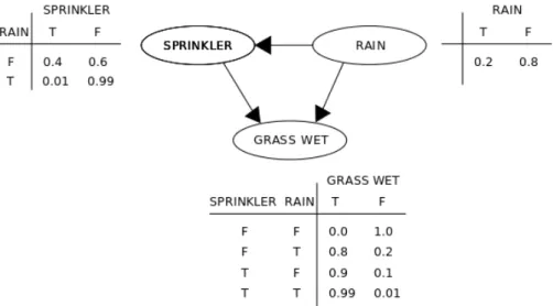
Figure 3.1: Simple Bayesian network and its probability tables. Public domain image.

3.1.3 Non-linear models

Some non-linear models are known to be easy to interpret and have a good reputation in industry.

Bayesian networks

Bayesian networks [Heckerman et al., 1995, Jensen and Nielsen, 2007, Friedman et al., 2000] model the covariates and their conditional dependencies via a Directed Acyclic Graph (DAG). Such an orientation is very user-friendly because it is similar to the way we imag-ine causality. But it is only about conditional dependencies. The usual example is the case of wet grass in a garden. You do not remember if the sprinkler was on or off and you do not know if it has rain.Then you look at the grass in your neighbour’s garden and it is not wet . . .

You will deduce that your sprinkler was on. Such conditionals dependencies are used in chapter 9 when confronted to missing values.

Figure 3.1.3 illustrates a simpler case with dependency between the sprinkler acti-vation and rain. It also shows probability tables associated to the Bayesian network. Bayesian networks are quite good in terms of interpretation because of that graphical and oriented representation of conditional probabilities. But they suffer from great dimension (combinatory issue) and require to transform the dataset arbitrary (discretisation), that imply a loss of information and usage of a priori (that is explicitly not suitable in our industrial context). The choice of the way to discretise the dataset has a great impact on the results and nothing can help if you have no a priori on the result you want to obtain. Computation relies on a table that describes all possible combinations for each covariate. Hence it is extremely combinatory if the graph has too much edges or is not sparse enough. Moreover, you need to define the graph before computing the bayesian network and without a priori it can be challenging and time consuming.

The concept of representing dependencies with directed acyclic graph is good an we keep it in our model. Thus we will keep the ease of interpretation.

(28)

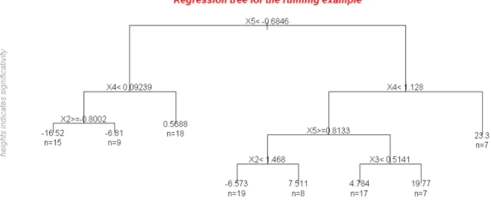
Figure 3.2: Regression tree obtain with the package CorReg (graphical layer on top of the rpart package) on the running example.

Classification and Regression Trees (cart)

Classification And Regression Trees (cart) [Breiman, 1984] are extremely simple to use and interpret, can work simultaneously with quantitative and qualitative covariates and are very fast to compute. They consist in recursive partitioning of the sample according to binary rules on the covariate (only one at a time) to obtain a hierarchy defined by simple rules and containing pure leaves (same value). It is followed by a pruning method to obtain leaves that are quite homogeneous and described with simple rules.

cart are implemented in the package rpart for R, on cran ([Therneau et al., 2014]). Our CorReg package offers a function to compute and plot the tree in one command with a subtitle to explain how to read the tree and global statistics on the dataset. But it is not convenient for linear regression problems as we see in figure 3.3 because a same variable will be used several times and the tree will fail to give a simple interpretation as “Y and

X1 are proportional”. Trivial case: Y = X1+ ÁY where ÁY ≥ N (0, ‡2YIn) with ‡2Y = 0.5. So cart will be used as a complementary tool for datasets with both quantitative and qualitative covariates or when the dependence between Y and X is not linear. We will focus our research on linear models with only quantitative variables.

Apart from linear models, the main issues are the lack of smoothness (prediction function with jumps) and especially instability because of the hierarchical partitioning. Modifying only one value in the dataset can impact a split and then change the range of possible splits in the resulting sub-samples so if a top split is modified the tree can be widely changed. Random Forests are a way to solve this problem and can be seen as a cross-validation method for regression trees. More details in the book from Hastie [Hastie et al., 2009].

(29)

(a) Tree found for the trivial case (b) True linear regression and splits obtained by the tree.

Figure 3.3: Predictive model associated to the tree (red) and true model (black)

3.2 Parameter estimation

3.2.1 Maximum likelihood and Ordinary Least Squares (ols)

We note the linear regression model:

Y = X— + ÁY (3.2)

where X is the n ◊ d matrix of the explicative variables, Y the n ◊ 1 response vector and ÁY ≥ N (0, ‡Y2In) the noise of the regression, with In the n-sized identity matrix and ‡Y > 0. The d ◊ 1 vector — is the vector of the coefficients of the regression. Thus we suppose that Y linearly depends on X and that the residuals are Gaussian and i.i.d. We also suppose that X has full column rank d. — can be estimated by ˆ— with Ordinary Least Squares (ols), that is the unbiased maximum likelihood estimator [Saporta, 2006, Dodge and Rousson, 2004]:

ˆ

—_OLS = (XÕX)≠1XÕY (3.3)

with variance matrix

Var(ˆ—OLS) = ‡2Y (XÕX)≠1. (3.4) In fact it is the Best Linear Unbiased Estimator (BLUE). The theoretical mse is given by

mse(ˆ—OLS) = ‡Y2 Tr((XÕX)≠1).

Equation (3.2) has no intercept but usually a constant is included as one of the regressors. For example we can take X1 _{= (1, . . . , 1)}_Õ_{. The corresponding element of — is then the}

intercept —1. In the following we do not consider the intercept to simplify notations. In

practice, an intercept is added by default.

Estimation of Y by ols can be viewed as a projection onto the linear space spanned by the regressors X that minimizes the distance with each individual (Xi, Yi) as shown in figure 3.4. It can be written

ˆ

(30)

Figure 3.4: Multiple linear regression with Ordinary Least Squares seen as a projection on the d≠dimensional hyperplane spanned by the regressors X. Public domain image.

Estimation of — requires the inversion of XÕ_X _{which will be ill-conditioned or even}

singular if some covariates depend linearly from each other. For a given number n of individuals, conditioning of XÕ_X _{get worse based on two aspects:}

• The dimension d (number of covariates) of the model (the more covariates you have the greater variance you get)

• The correlations within the covariates: strongly correlated covariates give bad-conditioning and increase variance of the estimators .

When correlations between covariates are strong, the matrix (XÕ_X₎≠1 is ill-conditioned

and the variance of ˆ—OLS increases (equation (3.4)), giving unstable and unusable es-timator [Hoerl and Kennard, 1970]. Another problem is that matrix inversion requires to have more individuals than covariates (n Ø d). When matrices are not invertible, classical packages like the function lm of R base package [R Core Team, 2014] use the Moore-Penrose pseudoinverse [Penrose, 1955] to generalize ols.

Last but not least, Ordinary Least Squares is unbiased but if some —i are null (irrele-vant covariates) the corresponding ˆ—i will only asymptotically tend to 0 so the number of covariates in the estimated model remains d. This is a major issue because we are search-ing for a statistical tool able to work without a priori on a big dataset containsearch-ing many irrelevant covariates. Pointing out some relevant covariates and how they really impact the response is the main goal here. We will need a variable selection method one moment or another. It could be as a pre-treatment (to run a first tool to select relevant covariates and then estimate the values of the non-zero coefficients) , during coefficient estimation (some estimators can lead to exact zeros in ˆ—) or by post-treatment (by thresholding with tests of hypothesis, etc.).

(31)

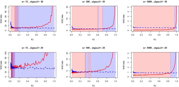
Figure 3.5: Evolution of observed Mean Squared error on ˆ—OLS with the strength of the correlations for various sample sizes and strength of regression. d = 5 covariates (running example).

Running example: We look at a simple case with d = 5 variables defined by four

independent scaled Gaussian N (0, 1) named X1_{, X}2_{, X}4_{, X}5 _{and X}3 _{= X}1 _{+ X}2 _{+ Á} 1

where Á1 ≥ N (0, ‡12In). We also define two scenarii for Y with — = (1, 1, 1, 1, 1)Õ and

‡Y œ {10, 20}. So there is no intercept (can be seen as a null intercept). It is clear that

XÕX will become more ill-conditioned as ‡1 gets smaller. In the following, the R2 stands

for the coefficient of determination which is here:

R2 = 1 ≠ Var(Á1)

Var(X3₎ (3.5)

Many other estimation methods were created to obtain better estimations by playing on the bias/variance trade-off or by making additional hypotheses. To have an easier comparison, we look at the empiric mse obtained on ˆ—.

Results shown in Figure 3.5 were obtained with usage of QR decomposition to inverse matrices, that is less impacted by ill-conditioned matrices [Bulirsch and Stoer, 2002] and used in the lm function from R to compute ols. But the correlations issue remains. Our package CorReg also uses this decomposition. We show the mean obtained after 100 ex-periences computed on our running example with validation sample of 1 000 individuals. The mse does explode with growing values of R2_{. The results confirm that the situation}

gets better for large values of n but strong correlations can still make the mse exploding. The variance of ˆ— is proportional to ‡2

Y so the mse are bigger when the main regression is weak (as in the real life).

3.2.2 Ridge regression: a penalized estimator

We have seen that ols is the Best linear Unbiased Estimator for ˆ—, meaning that it has the minimum variance. But it remains possible to play with the bias/variance trade-off

(32)

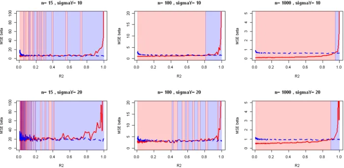
Figure 3.6: Evolution of observed Mean Squared error on ˆ—ridge with the strength of the correlations for various sample sizes and strength of regression. d = 5 covariates.

to reduce the variance by adding some bias. The underlying idea is that a small bias and a small variance could be preferred to a huge variance without bias. Many methods do this by a penalization on ˆ—.

Ridge regression [Hoerl and Kennard, 1970, Marquardt and Snee, 1975] proposes a possibly biased estimator for — that can be written in terms of a parametric L2 penalty:

ˆ

—= argmin_—Ó_{Î Y ≠ X— Î}2₂Ô subject to Î — Î2₂_{Æ ÷ with ÷ > 0} (3.6)

But this penalty is not guided by correlations. It introduces an additional parameter ÷ to choose for the whole dataset whereas correlations may concern only some of the covariates with several intensities.

The solution of the ridge regression is given by ˆ— = (XÕ_X_{+ ⁄I}

n)≠1XÕY (3.7)

and we see in this equation that a global modification of XÕ_X _{(on its diagonal) is done}

for a given ⁄ > 0 to improve its conditioning. Methods do exist to automatically choose a good value for ⁄ [Cule and De Iorio, 2013, Er et al., 2013] and a R package called ridge is on cran [Cule, 2014]. We have computed the same experiment as in previous figure but with the ridge package instead of ols. It is clear that the ridge regression is effi-cient in variance reduction (it is what it is built for). Moreover, ridge allows to have n < d. Like ols, coefficients tend to 0 but do not reach 0 so it gives difficult interpretations for large values of d. Ridge regression is efficient to improve conditioning of the estimator but gives no clue to the origin of ill-conditioning and keep irrelevant covariates. It remains a good candidate for prediction-only studies. Our industrial context makes necessary to have a variable selection method so we look further.