HAL Id: hal-00265346
https://hal.archives-ouvertes.fr/hal-00265346
Submitted on 19 Mar 2008
HAL is a multi-disciplinary open access
archive for the deposit and dissemination of
sci-entific research documents, whether they are
pub-lished or not. The documents may come from
teaching and research institutions in France or
abroad, or from public or private research centers.
L’archive ouverte pluridisciplinaire HAL, est
destinée au dépôt et à la diffusion de documents
scientifiques de niveau recherche, publiés ou non,
émanant des établissements d’enseignement et de
recherche français ou étrangers, des laboratoires
publics ou privés.
Athermal dynamics of strongly coupled stochastic
three-state oscillators
Bastien Fernandez, Lev Tsimring
To cite this version:
Bastien Fernandez, Lev Tsimring. Athermal dynamics of strongly coupled stochastic three-state
oscil-lators. Physical Review Letters, American Physical Society, 2008, 100 (16), pp.165705. �hal-00265346�
Athermal dynamics of strongly coupled stochastic three-state oscillators
Bastien Fernandez1 and Lev S. Tsimring2
1
Centre de Physique Th´eorique CNRS, Universit´es de Marseille I et II et de Toulon-Var,
Luminy Case 907, 13288 Marseille CEDEX 09, France
2 Institute for Nonlinear Science, University of California, San Diego, La Jolla, CA 92093-0402
We study the collective behavior of a globally coupled ensemble of cyclic stochastic three-state systems with transition rates from state i − 1 to state i proportional to the number of systems already in state i. While the mean field theory predicts only decaying oscillations in this system, direct numerical simulations indicate that the mean field exhibits stochastic oscillations even in the limit of large number of oscillators. We characterize the regularity of oscillations by the coherence parameter which has a well-defined maximum at the coupling constant of order 1. In contrast, the order parameter characterizing the level of synchrony among oscillators, increases monotonously with the coupling strength. We derive the exact solution of the full master equation for the stationary probability distribution and find the analytical expression for the order parameter.
PACS numbers:
Interacting stochastic systems emerge in a variety of physical and biological contexts, from arrays of Joseph-son junctions [1] and laser arrays [2] to neural networks [3, 4] and gene regulatory networks [5, 6]. While the dynamics of individual elements can be rather compli-cated and non-generic, the dynamics of a large ensem-ble of coupled units often exhibits universal behavior. Therefore, studies of canonical models with simple indi-vidual dynamics and interaction rules have proven very useful for understanding the behavior of specific systems. Well-known examples of such canonical systems are the Desai-Zwanzig model [7] of coupled bistable systems and the Kuramoto model [8] of coupled phase oscillators. The Kuramoto model and its many variations and generaliza-tions (see [9]) have been very successful in describing the transition to coherent oscillations in ensembles of coupled phase oscillators. Stochastic dynamics of individual ele-ments in such models are described by coupled nonlinear Langevin equations. In the thermodynamic limit, they can be reduced to low-dimensional deterministic equa-tions for the mean field or the order parameter charac-terizing global behavior of large systems.
A simpler way of describing interacting stochastic sys-tems incorporates stochastic elements with a discrete set of states with certain transition rates. It is most often done for bistable systems which are replaced by two-state stochastic systems with suitably chosen transition rates. For example, array-enhanced stochastic resonance has been studied in a system of globally coupled two-state systems [10]. A transition to regular oscillations in an ensemble of two-state systems coupled through a delayed mean field was studied in [11].
Recently, Prager et al. [12] introduced a globally
coupled three-state stochastic “oscillators” with uni-directional (1 → 2 → 3 → 1) transitions as a para-digmatic model of noise-driven excitable systems. This model is simple enough to make analytical and large-scale numerical studies of large systems feasible [12, 13]. An
important property is their behavior in the thermody-namic limit, when the number of units approaches infin-ity. Prager et al. [12] considered Markovian systems with transition rates depending on the suitably defined mean field and found no Hopf bifurcation in the thermody-namic limit. Instead, they found oscillations in this limit if the transitions between states are characterized by exponential waiting time distributions which imply non-Markovian dynamics. Later, Wood et al. [13] studied the dynamics of both globally and locally coupled Markovian three-state systems in the thermodynamic limit and did find a supercritical Hopf bifurcation to coherent periodic oscillations for strong enough coupling. While the indi-vidual systems considered in [12] and [13] were essentially identical, the difference between the models was in the way the coupling between the systems was introduced.
In this Letter we focus on the seemingly “less interest-ing” situation when the Markovian dynamics of a globally coupled ensemble of three-state systems does not exhibit a Hopf bifurcation. However, we find that in any finite-size system, quasi-regular oscillations of the mean field are present. We introduce the coherence parameter which characterizes regularity of mean field oscillations, and the order parameter which characterizes the degree of syn-chrony among the oscillators. We show that while the order parameter increases monotonously with the cou-pling strength, the coherence parameter has a maximum at a certain intermediate coupling strength. The simplic-ity and a high degree of symmetry in the system under study allow us to find the statistical properties of the finite ensemble analytically.
A single stochastic three-state unit with unidirectional transitions is schematically shown in the inset to Fig. 1b. We assume that in an isolated unit all three transitions from state i (i = 1, 2, 3) to state i + 1(mod3) are Markov-ian with identical rate a [14]. Without loss of generality we take a = 1. Statistical properties of this system have been investigated in Ref. [12]. The cyclic behavior of a
2 single oscillator is characterized by the mean time T of
an oscillator to return to the initial state after an excur-sion through the other two states. Since the mean time
of switching from state i to state i + 1 is Ts = 1, we
get T = 3Ts= 3. The probability for a system to be in
state i = 1, 2, 3 at time t is given by the continuous-time master equation
˙
Pi= −Pi+ Pi−1, i = 1, 2, 3 (1)
This master equation has a fixed point Ps
1 = P2s =
Ps
3 = 1/3 corresponding to equipartition among the
three states, and three eigenvalues λk = −1 + e2iπk/3,
k = 0, 1, 2. The first eigenvalue (k = 0) corresponds to the conservation of the total probability, and the other two describe equilibration of the probability distribution among the three states. Imaginary part of these eigenval-ues implies that there are decaying periodic oscillations of deviations from equipartition with the mean frequency
ω =√3/2.
Globally coupled three-state oscillators. Now let us
consider an ensemble of N identical three-state oscilla-tors. The specific mechanism of coupling is the
follow-ing. We assume that the probability πi,i+1 of
switch-ing of an oscillator from a state i to state i + 1 at time t is linearly proportional to the number of oscillators
ni+1(t) already at state i + 1 at time t, with the
propor-tionality constant b (which we call coupling coefficient), πi,i+1(t) = 1+b ni+1(t). This type of coupling is
reminis-cent of the auto-catalytic transitions in gene regulatory circuits when multiple copies of a single gene are present in the cell.
Since this model is Markovian, it can be efficiently
sim-ulated using Gillespie algorithm [15]. Figure 1 shows
sample stochastic trajectories for the occupation number of oscillators in states 1,2, and 3 as a function of time for different values of coupling parameter b for N = 1000.
The initial condition for all cases is n1(0) = N, n2,3(0) =
0. For b = 0, the population slowly drifts toward an
equi-librium state with n1 = n2 = n3 = N/3 with O(N1/2)
stochastic fluctuations. For even very small non-zero
b 1, noisy oscillations around the mean become visible. As b grows, the period becomes shorter, and the ampli-tude of oscillations grows until for b ∼ 1 it approaches N , i.e. almost all oscillators are simultaneously in the same
state. At large b 1, the system exhibits switching
behavior resembling the dynamics of a single oscillator. It is easy to understand: at very large b, once a single oscillator makes a transition from state i to state i + 1 (which occurs with rate N ), all other oscillators quickly follow. So indeed in the limit b 1 the dynamics of the ensemble becomes equivalent to the dynamics of a sin-gle oscillator with a rescaled transition rate N , a result confirmed by analytical calculations [20].
We computed the power spectrum of the time series of the occupation numbers and determined the central fre-quency ω and the half-width ∆ω of the spectral peak. We
0 50 100 150 200 250 300 0 200 400 600 800 1000 100 150 200 250 300 0 200 400 600 800 1000 100 125 150 0 200 400 600 800 1000 0 1 2 3 4 5 0 200 400 600 800 1000 a b c d (0,1,0) a a (0,0,1) (1,0,0) a
FIG. 1: Time series of the instantaneous occupation numbers oscillators n1, n2, n3in states 1, 2, 3 respectively for N = 1000,
and different values of the coupling parameter: (a) b = 0, (b) b = 0.1 (Inset: Transition diagram in a single unit); (c) b = 1, (d) b = 10.
call the ratio CP=ω/∆ω the coherence parameter. Fig-ure 2a shows ω, ∆ω, and CP as functions of the coupling parameter b. Both ω and ∆ω increase with b, however the coherence parameter has a distinct maximum at b ≈ 1, see Fig. 2a. This value appears to be independent of N for large enough N . Thus, we observe a manifestation of the coherence resonance [16], however the difference is that the maximum appears not at a certain noise strength but a certain value of the coupling.
This coherence resonance should not be confused with synchronization among the oscillators. The degree of syn-chronization can be characterized by the order parameter
R = * N−1 N X j=1 eiφj 2 + (2)
with discrete phases of oscillators φj= 2πk/3, k = 1, 2, 3.
This order parameter was introduced by [13] by anal-ogy with coupled continuum phase oscillators in the Ku-ramoto model [8]. The order parameter is zero when all oscillators are equally distributed among the three states
(n1 = n2 = n3 = N/3), and it approaches unity if all
oscillators are perfectly synchronized, so all of them are simultaneously in the same state. As expected, the order parameter increases monotonously with b, see Fig. 2b. As Figure 2b shows, the order parameter for a given b is independent of the number of oscillators in population N .
Mean-field approximation. In the thermodynamic limit N → ∞ of globally coupled oscillators, the mean-field equations for the deterministic “concentrations” of
oscil-lators xi= ni/N are given by
˙
xi= xi−1(1 + bN xi) − xi(1 + bN xi+1), i = 1, 2, 3(mod3)
(3) From the symmetry of the underlying dynamics it im-mediately follows that the fixed point of this system is
x1= x2= x3= 1/3. The associated two complex
eigen-values (the first eigenvalue is 0 as before because of the
conservation law) λ2,3= −32± i
√
0.01 0.1 1 10 100 b 0 0.2 0.4 0.6 0.8 1 ω, ∆ω , CP ω ∆ω CP/10 0.1 1 10 100 b 0 0.2 0.4 0.6 0.8 1 R N=102 N=103 N=104
FIG. 2: Gillespie simulations of coupled stochastic oscilla-tors: (a) mean frequency ω (blue squares), bandwidth ∆ω (black diamonds), and the coherence parameter CP (red cir-cles) vs. b for N = 100. (b) Order parameter R vs. b for N = 102, 103, 104. Solid line corresponds to formula (8).
negative real part, which indicates the absence of Hopf bifurcation at any coupling b. This is in contrast with the model by Wood et al. [13], in which a different form of coupling was proposed (the transition rate from i to i + 1 was an exponential function of the linear combination of
ni±1, ni), for which the mean field had a Hopf bifurcation
at large enough coupling strength [17].
Stochastic description. The full description of the sto-chastic properties of the system is given by the master
equation for the probability p(n1, n2, n3) that at time t
there are n1 oscillators at state 1, n2 at state 2, and n3
at state 3 (obviously, n1+ n2+ n3= N ), ˙ p(n1, n2, n3) = (n1+ 1)[1 + b(n2− 1)]p(n1+ 1, n2− 1, n3) +(n2+ 1)[1 + b(n3− 1)]p(n1, n2+ 1, n3− 1) +(n3+ 1)[1 + b(n1− 1)]p(n1− 1, n2, n3+ 1) −[N + b(n1n2+ n2n3+ n3n1)]p(n1, n2, n3)(4)
The total number of states (n1, n2, n3) in this system is
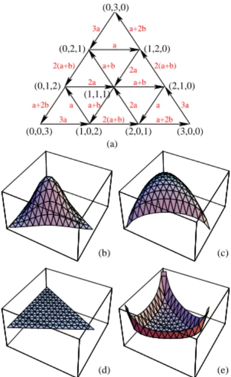
(N + 2)(N + 1)/2. It is convenient to depict the state space as a triangular grid, see Figure 3a.
According to the Frobenius-Perron Theorem, the mas-ter equation has a unique stationary solution. We were able to find the exact solution in a closed form,
ps(n1, n2, n3) = Cb G(b, n1)G(b, n2)G(b, n3) n1!n2!n3! (5) where G(x, n) = n−1 Y k=0
(1 + kx) and Cb is the
normaliza-tion constant, which can be verified by direct substitu-tion. Expression (5) shows that the stationary solution is not only invariant with respect to cyclic permutations but also with respect to any permutation of coordinates
(n1, n2, n3). This property is remarkable because the
equation itself does not possess this symmetry.
It is easy to check by direct substitution that (5) sat-isfies the relation
(n3+ 1)[1 + b(n1− 1)]ps(n1− 1, n2, n3+ 1) = n1(1 + bn3)ps(n1, n2, n3) (6) a+b (0,3,0) (0,2,1) (0,1,2) (0,0,3) (1,0,2) (2,0,1) (3,0,0) (2,1,0) (1,2,0) (1,1,1) (a) a+b 2(a+b) a 2a a+2b 3a 3a 2(a+b) 2(a+b) a+2b a+2b 3a a a 2a 2a a+b (e) (b) (d) (c)
FIG. 3: (a)State space of the three-oscillator system N = 3; correspond to distinct states (n1, n2, n3) of the system, and
arrows indicate transitions among the states. Expressions at the arrows show the corresponding transition rates. (b-e) Sta-tionary probability distributions for N = 14 and b = 0.2 (b), b = 0.8 (c), b = 1 (d) , b = 2 (e).
and two other relations obtained from (6) by cyclic per-mutations (adding these 3 relations and using the ro-tation symmetry gives the sro-tationary master equation equation (4) without l.h.s.).
It is straightforward to obtain convexity properties of
the stationary solution (5). Indeed, according to (6),
we have ps(n1 − 1, n2, n3 + 1) < ps(n1, n2, n3) iff 0 <
(n3+ 1 − n1)(1 − b). If b < 1 (resp. b > 1) the probability
increases (resp. decreases) when one moves one step to the right in the left part of the triangular lattice and vice versa [18]. Combining it with the rotation symmetry, we conclude that the distribution is convex with a maximum in the center when b < 1 and concave with a maximum in the corners for b > 1; for b = 1 the distribution is flat. For zero coupling (b = 0), the stationary distribution is trinomial
ps(n1, n2, n3) =
N ! 3Nn
1!n2!n3!
which of course could be deduced directly since oscillators are independent and in the long term limit they become uniformly distributed among the three states. The most
probable state is in the middle of the triangle (n1= n2=
n3= N/3) and the least probable states are in the corners
(N, 0, 0), (0, N, 0), (0, 0, N ).
For large b, the stationary distribution is highly local-ized at the corners. However there is a small (O(1/b)) probability flux in and out of the corners. In the first
4 order of 1/b, the stationary probability distribution is
ps(n, 0, N − n) = N 3bn(N − n)+ O(1/b 2), n = 1, N − 1 ps(0, 0, N ) = 1 3 − 2 3b N −1 X k=1 1 k+ O(1/b 2)
(the remaining state probabilities follow from cyclic per-mutation) and ps(n1, n2, n3) = O(1/b2) for n1n2n36= 0.
Thus the probability distribution has a deep minimum at the center of the triangle, and sharp peaks in the
corners (Fig. 3e). The dynamics close to equilibrium
can be approximated by the probability flow around the edges of the triangle, ignoring the influence of the inner nodes. This simplification allows us to compute the non-zero eigenvalues of the full system in the first order in 1/b [20]. As expected, for large b these eigenvalues are
λkN + O(1/b2), k = 1, 2, where λk are the eigenvalues
of the single oscillator. It is interesting to note that the
equilibration rate Re(−λ1,2N ) is independent of b.
For large n1, n2and n3one can use Stirling formula to
find an asymptotic expression for the distribution (5), ps(n1, n2, n3) = Cb
bN
Γ3(1/b)(n1n2n3)
1/b−1 (7)
with Cb = b−NΓ(3/b)Γ−2(1/b)N1−2/b. We can use this
expression, replace summation by integration and com-pute the order parameter for large N explicitly [19]. This straightforward calculation results in a surprisingly sim-ple formula
R = b
b + 3 (8)
This formula agrees very well with direct Gillespie sim-ulations (Fig. 2b). Note that the order parameter is independent of N (at least for large N ). For arbitrary N , the order parameter can be computed from the sta-tionary distributions at zero coupling and large coupling respectively. For zero coupling, we get R = 1/N and for
large coupling, we have R = 1 −3b(1 −N1) + O(1/b2).
Discussion. Our analysis indicates that in the system of globally coupled three-state units there are significant stochastic oscillations, and while the frequency of these oscillators scales as N , their temporal coherence reaches maximum at a finite b ∼ 1 independent of the number of oscillators. This result is counterintuitive, since the mean-field theory predicts no sustained oscillations in the thermodynamic limit N → ∞. The origin of this apparent contradiction is that for sufficiently large cou-pling strength, the implicit assumption of decorrelated dynamics of individual noisy units is violated. For b ∼ 1, the transition rate of the “last” oscillators remaining in state i when most of them are already in state i + 1, is large, O(N ), and so the transitions of these “last” oscil-lators are strongly correlated. For large b, all osciloscil-lators are strongly correlated: as soon as the first one makes a transition, the rest very quickly follows. This leads to
the correlated and thus athermal behavior of the globally coupled system at large b. Of course, in any real system the transition rate should saturate as N → ∞. Then eventually the thermal behavior of the system would be recovered, however in the intermediate scaling regime of finite N the dynamics described here can be observed. Note that our results are easily generalizable to the case of arbitrary p-state oscillators with any p > 2. The
or-der parameter for p-oscillators is simply Rp= b/(b + p),
and the coherence parameter reaches maximum at b ∼ 1. However, the behavior of boolean systems (p = 2) is dif-ferent: while the order parameter still exhibits the same
behavior (R2 = b/(b + 2)), the quasi-regular oscillations
are completely absent, and the coherence parameter re-mains small O(1) throughout the full range of b.
Authors are indebted to K. Lindenberg for an illumi-nating discussion, and to the anonymous referee for a suggestion to consider arbitrary p-state oscillators. LT is grateful to CNRS and to University of Aix-Marseille I for hospitality and support. This work was partially sup-ported by ACI IMPBio (BF) and MURI and NIH (LT)
[1] P. Hadley, M. Beasley, and K. Wiesenfeld, Phys. Rev. B 38, 8712 (1988).
[2] H. Bruesselbach, D. Jones, M. Mangir, M. Minden, and J. Rogers, Opt. Lett. 30, 1339 (2005).
[3] M. Abeles, Corticonics: Neural Circuits of the Cerebral Cortex (Cambridge University Press, 1991).
[4] M. Tsodyks, K. Pawelzik, H. Makram, Neural Comp. 10, 821 (1998).
[5] J. Hasty, J. Pradines, M. Dolnik, and J. Collins, PNAS 97, 2075 (2000).
[6] J. Paulsson, Nature 427, 415 (2004).
[7] R. Desai and R. Zwanzig, J. Stat. Phys. 19, 1 (1978). [8] Y. Kuramoto, Chemical oscillations, waves, and
turbu-lence (Springer-Verlag, 1984).
[9] J. Acebr´on, L. Bonilla, C. P´erez Vicente, F. Ritort, and R. Spigler, Reviews of Modern Physics 77, 137 (2005). [10] J. Lindner, M. Bennett, and K. Wiesenfeld, Phys. Rev.
E 73, 031107 (2006).
[11] D. Huber and L. Tsimring, Phys. Rev. Lett. 91, 260601 (2003).
[12] T. Prager, B. Naundorf, and L. Schimansky-Geier, Phys-ica A 325, 176 (2003).
[13] K. Wood, C. Van den Broeck, R. Kawai, and K. Linden-berg, Phys. Rev. Lett. 96, 145701 (2006); Phys. Rev. E 74, 031113 (2006); 75, 041107 (2007); Physical Review E 76, 041132 (2007).
[14] This assumption is made merely for analytical tractabil-ity, the behavior remains qualitatively the same for non-equal transition rates.
[15] D. Gillespie, J. Phys. Chem. 81, 2340 (1977).
[16] A. Pikovsky and J. Kurths, Phys. Rev. Lett. 78, 775 (1997).
[17] For a general nonlinear transition probability πi,i+1 =
Π(xi+1), the real part of the eigenvalues is given by
[Π0(1/3) − 3Π(1/3)]/2, so the Hopf bifurcation
Π0(1/3)/Π(1/3) can exceed 3.
[18] The left part of the lattice corresponds to points for which N1≤ N3− 1.
[19] When N is large, the states (n1, n2, n3) close to the edges,
where the expression (7) is not valid, give a little
contri-bution to the order parameter.
[20] See EPAPS Document No. [XX] for details of first order in 1/b eigenvalues computation.