HAL Id: hal-01457892
https://hal.archives-ouvertes.fr/hal-01457892
Submitted on 6 Feb 2017
HAL is a multi-disciplinary open access
archive for the deposit and dissemination of
sci-entific research documents, whether they are
pub-lished or not. The documents may come from
teaching and research institutions in France or
L’archive ouverte pluridisciplinaire HAL, est
destinée au dépôt et à la diffusion de documents
scientifiques de niveau recherche, publiés ou non,
émanant des établissements d’enseignement et de
recherche français ou étrangers, des laboratoires
On planar right groups
Kolja Knauer, Ulrich Knauer
To cite this version:
Kolja Knauer, Ulrich Knauer. On planar right groups. Semigroup Forum, Springer Verlag, 2016, 92,
pp.142 - 157. �10.1007/s00233-015-9688-2�. �hal-01457892�
On planar right groups
Kolja Knauer
Ulrich Knauer
January 7, 2015
Abstract
In 1896 Heinrich Maschke characterized planar finite groups, that is groups which admit a generating system such that the resulting Cayley graph is planar. In our study we consider the question, which finite semi-groupshave a planar Cayley graph. Right groups are a class of semigroups relatively close to groups. We present a complete characterization of pla-nar right groups.
1
Introduction
Cayley graphs of groups and semigroups enjoy a rich research history and are a classic point of interaction of Graph Theory and Algebra. While on the one hand knowledge about the group or semigroup gives information about the Cayley graph, on the other hand properties of the Cayley graph can be translated back to the algebraic objects and their attributes. A particular use of Cayley graphs is simply to visualize a given group or semigroup by drawing the graph. It is therefore interesting to find Cayley graphs that can be drawn respecting certain aesthetic, geometric or topological criteria and then characterizing which groups or semigroups have Cayley graphs that can be drawn in such a way. Here we will focus on topological criteria, more precisely, on embeddability of the graph into orientable surfaces. The theoretic appeal of such type of question is that they now lie in the intersection of Graph Theory, Algebra, and Topology.
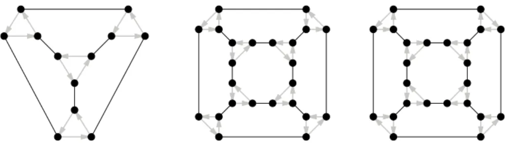
A group is called planar if it admits a generating system such that the resulting Cayley graph is planar, that is, it admits a plane drawing. See Figure 1 for examples. Finite planar groups were characterized by Maschke [13], see Table 1. There has been considerable work towards a characterization of infinite planar groups, see e.g. [5, 6].
With an analogous definition one might ask for planar semigroups. Zhang studied planar Clifford semigroups [17]. Solomatin characterized planar prod-ucts of cyclic semigroups [15] and described finite free commutative semigroups and some other types, which are outerplanar [16]. For this he uses his own planarity results, which are not easily accessible. We looked at toroidal right groups [11] but still no characterization is known. In the present paper we char-acterize planar right groups. Some of the results have already been announced in [12].
Figure 1: From left to right: the plane Cayley graphs Cay(A4, {(12)(34),(123)}),
Cay(S4, {(123), (34)}), and Cay(Z2× A4, {(0, (123)), (1, (12)(34))}).
In Section 2 we introduce first notions of Cayley graphs of semigroups. In Section 3 we review Maschke’s characterization of finite planar groups. In Sec-tion 4 we construct planar embeddings of those right groups which in the end will turn out to be exactly the planar ones. Section 5 we study how Cayley graphs of the group are reflected in the Cayley graph of a right group. In par-ticular, we reduce the set of right groups that have to be checked for planarity. In Section 6 we prove that all candidates for planar right groups not shown to be planar before are not planar and therefore conclude the characterization. We close the paper with stating the characterization Theorem 7.1 and a set of open problems in Section 7.
2
Preliminaries
Given a semigroup S and a set C ⊆ S we call the directed multigraph Cay(S, C) = (V, A) with vertex set V = S and directed arcs (s, sc) for all s ∈ S and c ∈ C the directed right Cayley graph or just the Cayley graph of S with connection set C. In drawings of Cayley graphs we will generally use different shades of gray for arcs corresponding to different elements of C. If a pair of vertices is connected by an arc in both directions we simply draw an undirected edge between them. See Figure 1 for an example.
The genus γ(M ) of an orientable surface M is its number of handles. The genus γ(Γ) of a (directed) graph Γ is the minimum genus over all surfaces it can be embedded in. The genus γ(S) of a semigroup S is the minimum genus over all Cayley graphs Cay(S, C) where C is a generating system of S. We say that S is planar if γ(S) = 0, i.e., there exists a generating set C of S such that Cay(S, C) has a crossing-free drawing in the plane.
Clearly, when considering genus we may ignore edge-directions, multiple edges and loops. We call the resulting simple undirected graph the underlying graph and denote it by Cay(S, C).
Given an undirected graph Γ and a subset E of the edges E(Γ) of Γ, the deletion of E in Γ, denoted by Γ \ E, is simply the graph obtained from Γ by suppressing all edges in E. Further, we denote by Γ/E the contraction of E in Γ. This is, the graph that arises from Γ by identifying vertices that are adjacent via an edge in E and deleting loops afterwards. A graph Γ′ is a minor of Γ if
Γ′ can be obtained by a sequence of deletions and contractions from Γ. If Γ′ is obtained only using deletions or only contractions, we say that Γ′ is a deletion-minor and contraction-deletion-minor, respectively. Similarly, one defines the notions of deletion, contraction, and minors in directed graphs.
Given a graph Γ we denote by Aut(Γ) its group of automorphisms and by End(Γ) its monoid of endomorphisms.
The contraction lemma due to Babai [1, 2] is the following:
Lemma 2.1. Let Γ be a connected graph and G < Aut(Γ). If the left action of G on Γ is fixpoint-free, then there exists E ⊂ E(Γ) and a generating set C of G such that Cay(G, C) ∼= Γ/E.
A directed graph is called strongly connected if for each pair u, v there is a directed path from u to v. Since for a minor Γ′ of Γ one generally has γ(Γ′) ≤
γ(Γ), we can apply Lemma 2.1 in order to obtain the following useful lemma: Lemma 2.2. Let S be a semigroup and C ⊆ S such that Cay(S, C) is strongly connected. Then for every subgroup G of S we have γ(G) ≤ γ(Cay(S, C)). Proof. For any g ∈ G and (s, sc) ∈ E(Cay(S, C)) by definition we have (gs, gsc) ∈ E(Cay(S, C)). Hence, g ∈ End(Cay(S, C)). Clearly, g−1is the inverse mapping
of g. Thus, g ∈ Aut(Cay(S, C)). To see that G acts fixpoint-free, suppose gs = s for some s ∈ S. Now for every out-neighbor sc of s we have gsc = sc, i.e., sc is also a fixpoint of g. Choose a directed path P from s to some h ∈ G. We obtain gh = h, which implies g = e. Hence the left action of G on Cay(S, C) is fixpoint-free. This implies that the same holds with respect to Cay(S, C). Thus, we may apply Lemma 2.1 and obtain some generating system, C′ of G
such that Cay(G, C′) is a contraction-minor of Cay(S, C). Since contraction
cannot increase the genus of a graph the claim follows.
The above works also for the infinite case. Nevertheless, we are only inter-ested in the finite case. So, Lemma 2.2 justifies to review the characterization of finite planar groups due to Maschke [13], which we will do in the next section.
3
Maschke’s Theorem – a closer look
Before stating the theorem let us introduce some standard group notation: Zn = {0, . . . , n − 1}. Note that Zm× Zn ∼= Zmn if gcd(m, n) = 1. In particular, Z2× Z2∼= D2.
Dn the dihedral group. The elements of Dn are the symmetries of the n-gon
with the vertices 1, . . . , n, that is |Dn| = 2n. By h13i we denote the reflection
around the axis through 2, by h12i the reflection around the axis through the middle line between 1 and 2. The rotation by 1 is denoted by (1 . . . n). Note that Z2× Dn∼= D2n, if n is odd.
An, Sn the alternating group and the symmetric group, respectively, on the
n points 1, . . . , n, n ≤ 5. For their elements we use the cycle notation.
The identity element is denoted by e for all groups G except for Zn, where
we rather use 0.
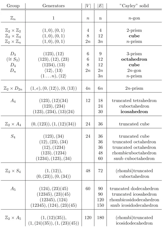
Theorem 3.1 (Maschke’s Theorem). The groups and minimal generating sys-tems in Table 1 are exactly those pairs having a planar Cayley graph.
Group Generators |V | |E| ”Cayley” solid Zn 1 n n n-gon Z2× Z2 (1, 0), (0, 1) 4 4 2-prism Z2× Z4 (1, 0), (0, 1) 8 12 cube Z2× Zn (1, 0), (0, 1) 2n 3n n-prism D3 (123), (12) 6 9 3-prism (∼= S3) (123), (12), (23) 6 12 octahedron D4 (1234), (13) 8 12 cube
Dn h12i, h13i 2n 2n 2n-gon
(1 . . . n), h12i 3n n-prism
Z2× D2n (1, e), (0, h12i), (0, h13i) 4n 6n 2n-prism
A4 (123), (12)(34) 12 18 truncated tetrahedron (123), (234) 24 cuboctahedron (123), (234), (13)(24) 30 icosahedron Z2× A4 (0, (123)), (1, (12)(34)) 24 36 truncated cube S4 (123), (34) 24 36 truncated cube (12), (23), (34) 36 truncated octahedron (12), (1234) 36 truncated octahedron (123), (1234) 48 rhombicuboctahedron (1234), (123), (34) 60 snub cuboctahedron Z2× S4 (1, (12)), 48 72 (rhombi)truncated (0, (23)), (0, (34)) cuboctahedron A5 (124), (23)(45) 60 90 truncated dodecahedron (12345), (23)(45) 90 truncated icosahedron (12345), (124) 120 rhombicosidodecahedron (12345), (124), (23)(45) 150 snub icosidodecahedron Z2× A5 (1, (12)(35)), 120 180 (rhombi)truncated (1, (24)(35)), (1, (23)(45)) icosidodecahedron Table 1: The planar groups, their minimal generating systems giving planar Cayley graphs, and the three-dimensional solids these graphs are the graphs of.
Figure 2: The two plane Cayley graphs Cay(A5, {(124), (23)(45)}) and
Cay(Z2× A5, {(1, (12)(35)),(1, (24)(35)),(1, (23)(45))}).
4
Planar right groups
The right zero band on k elements is the semigroup Rk on the set {r1, . . . , rk}
such that rirj := rj for all i, j ∈ [k], where through the entire paper we will
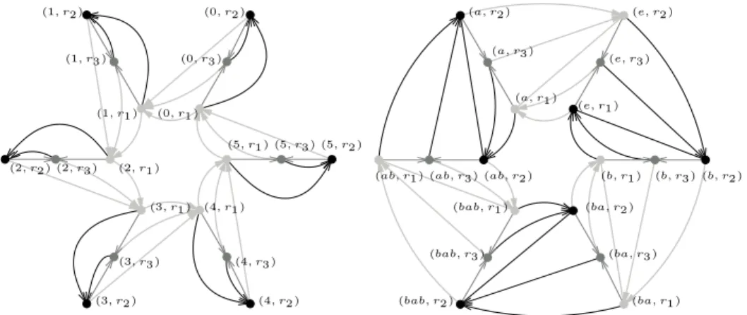
denote [k] := {1, . . . , k}. A semigroup S is called a right group if it is isomorphic to the product G × Rk of a group and a right zero band. See Figure 3 for
examples.
On the way to characterize planar right groups we start with positive results in this section. (0, r1) (1, r1) (2, r1) (3, r1) (4, r1) (5, r1) (0, r2) (1, r2) (2, r2) (3, r2) (4, r2) (5, r2) (0, r3) (1, r3) (2, r3) (3, r3) (4, r3) (5, r3) (e, r1) (b, r1) (a, r1) (ab, r1) (bab, r1) (ba, r1) (e, r2) (b, r2) (a, r2) (ab, r2) (bab, r2) (ba, r2) (e, r3) (b, r3) (a, r3) (ab, r3) (bab, r3) (ba, r3)
Figure 3: Plane Cayley graphs Cay(Z6 × R3, {(1, r1), (0, r2),(0, r3)}) and
Cay(D3 × R3, {(a, r1), (b, r2),(e, r3)})}. Vertex colors stand for G × {r1},
G × {r2}, andG × {r3}, respectively.
Remark 4.1. Analogously one considers a left zero band Lk = {l1, . . . , lk} on k
whose generating systems always have the form Lk× C where C is a generating
system of G. The right Cayley graph Cay(Lk× G, Lk× C) consists of k copies
of Cay(G, C). Consequently, a left group Lk × G is planar if and only if the
group G is planar, for arbitrary k ∈ N.
Lemma 4.2. If G ∈ {Zn, Dn} then G × R2 and G × R3 are planar.
Proof. If G = Zn with generator b then Cay(Zn, {b}) is a cycle. Now D :=
{(b, r1), (e, r2), (e, r3)} is a generating system of Zn× R3. A plane drawing of
Cay(Zn× R3, D) is on the left of Figure 3 for the case n = 6.
If G = Dn with two degree two generators a, b then again Cay(Dn, {a, b})
is a cycle and D := {(a, r1), (b, r2), (e, r3)} is a generating system of Dn× R3.
A plane drawing of Cay(Dn× R3, D) is shown on the right of Figure 3 for the
case n = 3.
Now, for G ∈ {Zn, Dn} and S′ := G × R2 note that D′ := D\{(e, r3)} is a
generating system of S′ and Cay(S′, D′) is a subgraph of Cay(S, D). Thus, it
is also planar.
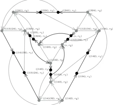
Lemma 4.3. Let G be a group with generating system C = {a, b} with a2 = e
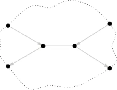
and b26= e. If Cay(G, C) has an embedding on a surface M such that for each
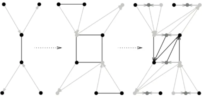
a-edge the b-arcs incident with it alternate in direction when ordered by the local rotation systems, see the left of Figure 4, then γ(G × R2), γ(G × R3) ≤ γ(M ).
Figure 4: Left: Local configuration of b-arcs (gray) around an a-edge (black). Middle: Topologically relevant part of the transformation. Right: Completion to graph of right group. Arc and vertex colors stand for elements of G × {r1}, G × {r2}, andG × {r3}, respectively.
Proof. We first show the statement for S := G × R3. As a generating system we
use D := {(a, r1), (b, r2), (e, r3)}. The property of our embedding of Cay(G, C)
on M makes it possible to blow up a-edges to rectangles such that incoming b-arcs are attached to one pair of opposite vertices and outgoing b-arcs to an entire side of the rectangle each, see the middle of Figure 4. This blown up graph can be completed to the wanted embedding of Cay(S, D). This is shown on the right of Figure 4.
For S′ := G × R
2 note that D′ := D\{(e, r3)} is a generating system of
S′ and Cay(S′, D′) is a subgraph of Cay(S, D). Thus, Cay(S′, D′) embeds in
M . An example for this construction in the case S′ := G × R
2 and G = A4 is
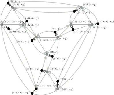
However, similarly one can see that choosing D′′ = {(e, r1), (a, r2), (b, r2)},
also yields a graph Cay(S′, D′′′) which can be embedded into M . This construc-tions for the case S′:= G × R2is exemplified with G = A4in Figure 6.
(e, r1) ((123), r1) ((132), r1) ((134), r1) ((142), r1) ((143), r1) ((241), r1) ((324), r1) ((324), r1) ((12)(34), r1) ((13)(24), r1) ((14)(32), r1) (e, r2) ((123), r2) ((132), r2) ((134), r2) ((142), r2) ((143), r2) ((241), r2) ((324), r2) ((324), r2) ((12)(34), r2) ((13)(24), r2) ((14)(32), r2)
Figure 5: The plane Cayley graph Cay(A4× R2, {((12)(34), r1),(123), r2))}).
This exemplifies the principal construction in Lemma 4.3 and generalizes to A4×R3. Vertex colors stand for elements of G×{r1} andG × {r2}, respectively.
Theorem 4.4. If G ∈ {{e}, Zn, Dn, S4, A4, A5} then G × Rk and {e} × Rk′ are
planar for k ≤ 3 and k′ ≤ 4.
Proof. For Zn and Dn this was proved in Lemma 4.2. For the remaining groups
this follows by their plane drawings provided in Figure 1 and Figure 2 and ap-plying Lemma 4.3. Moreover, Cay({e} × Rk′, Rk′) is isomorphic to the complete
graph on k′ vertices K
k′. Together this yields the claim.
It remains to show that the list of planar right groups in Theorem 4.4 is complete.
5
Planar right groups come from planar groups
For C ⊆ G × Rk we denote the projections of C on the respective factors by
πG(C) := {g ∈ G | ∃j ∈ [k] : (g, rj) ∈ C} and πRk(C) := {rj ∈ Rk | ∃g ∈ G :
(g, rj) ∈ C}. We start with the following basic lemma, which does not hold in
(e, r1) ((123), r1) ((132), r1) ((134), r1) ((142), r1) ((143), r1) ((241), r1) ((342), r1) ((324), r1) ((12)(34), r1) ((13)(24), r1) ((14)(32), r1) (e, r2) ((123), r2) ((132), r2) ((134), r2) ((142), r2) ((143), r2) ((241), r2) ((342), r2) ((324), r2) ((12)(34), r2) ((13)(24), r2) ((14)(32), r2)
Figure 6: The graph Cay(A4× R2, {(e, r1),((12)(34), r2),(123), r2))}). This
exemplifies the alternative construction for G × R2 mentioned in the proof of
Lemma 4.3. Vertex colors stand for elements of G × {r1} andG × {r2},
respec-tively.
Lemma 5.1. Let C ⊆ S = G × Rk, then the following are equivalent
(i) C generates S,
(ii) πG(C) generates G and πRk(C) generates Rk,
(iii) Cay(S, C) is strongly connected.
Proof. Clearly, (i) implies (ii). Now, we show (ii)⇒(iii): Take s = (g, ri), t =
(h, rj) ∈ S. Multiply s from the right by a sequence of elements of C in order
to obtain (h, rℓ) for some ℓ ∈ [n]. Now, take some (f, rj) ∈ C and multiply it
order of f many times to (h, rℓ) from the right. We obtain a directed path from
s to t. This yields that Cay(S, C) is strongly connected.
To see, (iii)⇒(i), let s ∈ S. Any directed path in Cay(S, C) from a vertex c ∈ C to s corresponds to a word of elements of C generating s. By strong connectivity, such a path exists.
Lemma 2.2 and Lemma 5.1 together yield that in our characterization we only need to consider planar groups as factors. Unfortunately, Lemma 2.2 does not preserve the generating system of the right group we start out from. Special-izing to right groups we can obtain a stronger statement under certain circum-stances. For this we introduce the notation πG(C)j := {g ∈ G | (g, rj) ∈ C}.
Lemma 5.2. Let S = G × Rk and C a generating set such that there exists
(g, rj) ∈ C with g−1hg = h±1 for all h ∈ πG(C)j or for all h ∈ πG(C)\πG(C)j.
Proof. Let (g, rj) ∈ C be the element claimed in the statement of the lemma.
Delete all arcs of the form (g′, ri), (g′f, rℓ) with f 6= g and i 6= ℓ. Contract
all arcs of the form ((g′, ri), (g′g, rj)) for i 6= j. Since every vertex (g′, ri)
with i 6= j has an arc of that form, we can view the new set of vertices as G × {rj}. In the contracted graph there is an arc ((g′, rj), (f, rj)) if it was
there before, i.e., there is (h, rj) ∈ C with g′h = f , or if it arose from the
contraction. In this case for some i 6= j there are ((g′g−1, r
i), (f g−1, ri)) and
(h, ri) ∈ C with g′g−1h = f g−1. This is, the new graph is isomorphic to
Cay(G, πG(C)j∪ g−1(Si6=jπG(C)i)g). We remove some further edges to obtain
Cay(G, πG(C)j∪ g−1(πG(C)\πG(C)j)g).
Now we use the assumption on (g, rj). If we have g−1hg = h±1 for all h ∈
πG(C)j, then Cay(G, πG(C)j∪g−1(πG(C)\πG(C)j)g) = Cay(G, (g−1πG(C)g)±1).
But since g′h = f ⇔ g−1g′gg−1hg = g−1f g we have that the contracted graph
Cay(G, (g−1π
G(C)g)±1) is isomorphic to Cay(G, πG(C)±1). This means that
Cay(G, πG(C)) is a minor of Cay(S, C).
If we have g−1hg = h±1 for all h ∈ π
G(C)\πG(C)j, then Cay(G, πG(C)j∪
g−1(π
G(C)\πG(C)j)g) = Cay(G, πG(C)±1). Hence, Cay(G, πG(C)) is a minor
of Cay(S, C).
Many right groups satisfy the preconditions for Lemma 5.2. Note for instance that if the group generated by some πG(C)jis Abelian, then the preconditions of
Lemma 5.2 are trivially satisfied. A Coxeter system is a group G with generating system C, such that all generators are of order 2 and all relations are of the form (cicj)mij = e. The Coxeter-Dynkin diagram of a Coxeter system is an (edge
labeled) graph, on the vertex set C, with an edge connecting ci and cj if and
only if mij ≥ 3. A consequence of the classification of finite Coxeter groups,
due to Coxeter [4] is that the Coxeter-Dynkin diagram of a Coxeter system is a tree.
Proposition 5.3. Let S = G × Rk and C a generating set. If (G, πG(C)) forms
a Coxeter system, then Cay(G, πG(C)) is a minor of Cay(S, C).
Proof. Let g ∈ πG(C)j be a leaf of the corresponding Coxeter-Dynkin diagram,
and h its neighbor. If the only i ∈ [k] with h ∈ πG(C)i is i = j, then (gf )2= e
for all f ∈ πG(C) \ πG(C)j and Lemma 5.2 gives the result. Otherwise we can
consider C′ := C \ {(h, r
j)}, which satisfies Lemma 5.1(ii) and therefore is still
generating. Moreover, Cay(G, πG(C′)) is a deletion minor of Cay(G, πG(C)).
We have that (gf )2= e for all f ∈ π
G(C′)j and Lemma 5.2 gives the result.
We believe, that a stronger form of Lemma 5.2 should hold.
Conjecture. Let S = G × Rk and C a generating set. Then Cay(G, πG(C)) is
a minor of Cay(S, C).
Note that for products G × S of group G and semigroup S not being a right zero band the natural generalization of the conjecture is false. Indeed, even if S = Z2 it is false: Consider the planar representation of A5× Z2 with three
generators of order two, see Figure 2. Since there is no planar representation of A5 with three generators of order two, no Cayley graph of A5 arising by
projecting the generating system of A5× Z2 to A5 is a minor of the planar
We will prove a weakening of this conjecture for the planar case in Theo-rem 5.6. Essentially we will prove, that in order to not satisfy the preconditions of Lemma 5.2 the Cayley graph must have too many edges to be planar. There-fore, we need the classic result of Euler:
Lemma 5.4 (Euler’s Formula). Every simple connected plane graph G with vertex set V , edge set E and face set F fulfills |V | − |E| + |F | = 2. In particular, G has at most 3|V | − 6 edges and at most 2|V | − 4 edges if the embedding has no triangular faces.
As a second ingredient we need a formula for the number of edges of the underlying undirected Cayley graph of a right group. For C ⊆ G × Rk and
a ∈ G we set ca:= |{j ∈ [k] | (a, rj) ∈ C}|. Furthermore set m := |G|.
Lemma 5.5. Let S = G × Rk with generating system C. Then Cay(S, C) has
km vertices and its number of edges is:
m(( X a∈πG(C) cak − ca−1 2 ) − ce 2) ≥ m 2 ((2k − 1) X a∈πG(C) ca− ce). (1)
Proof. The number of vertices is trivial.
We start by proving the equality for the number of edges. Every element (a, ri) ∈ C contributes an outgoing arc at every element of S. But if (a−1, rj) ∈
C all arcs of the form ((g, rj), (ga, ri)) are counted twice and there are m of
them. Note that this occurs in particular if a2 = e and also if i = j. So,
this yields mkca− ca−1
2 m edges labeled a. In the particular case that a = e
additionally at each vertex (g, ri) a loop can be deleted, i.e., instead of counting
half an edge at each such vertex we count none. This yields the −mce
2 in the
formula.
Together we obtain the claimed equality.
Observe now that for fixed ce the left-hand-side of the formula is minimized
if a2= e for every a ∈ π
G(C), i.e., ca= ca−1. This yields the lower bound.
Theorem 5.6. Let S = G × Rk and C a generating system such that Cay(S, C)
is planar. Then Cay(G, πG(C)) is a minor of Cay(S, C), i.e., in particular
planar.
Proof. The statement is trivial for k = 1 so assume k ≥ 2. If we cannot apply Lemma 5.2 we know in particular that |πG(C)j| > 1 for all j ∈ [k] and in
particularPa∈πG(C)ca ≥ 2k. Moreover, we have e /∈ πG(C). Thus ce= 0.
We can now use Lemma 5.5 to estimate the number of edges of Cay(S, C). Indeed, since ce= 0 we get the following lower bound from (1):
m
2(2k − 1) X
a∈πG(C)
ca≥ (2k − 1)mk > 3mk − 6, for k ≥ 2,
whereas the smallest value in this chain is the upper bound for the number of edges of a planar graph given by Lemma 5.4 – a contradiction.
6
Non-planar right groups from planar groups
In this section we show that the right groups Z2 × H × Rk with H any ofZ2(n+1), D2n, A4, S4, A5 where n ≥ 1 and k ≥ 2 are not planar. Moreover, {e} × Rk is not planar for k ≥ 5. Since Z2× Z2 ∼= D4, Z2× Z2n+1 ∼= Z4n+2
and Z2× D2n+1 ∼= D4n+2 for all n ≥ 1 this is exactly the set of right groups we
have to prove to be non-planar in order to show that the list from Theorem 4.4 is complete.
Euler’s Formula already allows us to restrict the size of the right zero band in the product of a planar right group:
Proposition 6.1. If G is nontrivial and G × Rk is planar, then k ≤ 3.
More-over, G × Rk is non-planar for any G and k ≥ 5.
Proof. Let k ≥ 4 and G × Rk with G non-trivial, i.e., there is a ∈ G such that
ca > 0. The lower bound in (1) is minimized if k = 4 and there is exactly one
such a ∈ G and ca = 1. In this case (1) gives m((3k −32) + (k − 12) − 32) =
12.5m > 12m − 6 – a contradiction to Euler’s Formula (Lemma 5.4).
Since Cay({e} × Rk, Rk) ∼= Kk and Kk is non-planar for all k ≥ 5 we obtain
the second part of the statement.
With some further edge counting we obtain:
Proposition 6.2. The right groups Z2× H × Rk with H any of D2n, S4, A5,
where n ≥ 1 and k = 2, 3, are not planar.
Proof. Let S = G × Rk be one of the right groups from the statement and
suppose that C is a generating system of S such that Cay(S, C) is planar. By Theorem 5.6 we know that there is a generating system C′ ⊆ π
G(C) of G
such that Cay(G, C′) is planar. Comparing with Table 1 we see that all planar
generating systems for our choice of G consist of three generators all having order two, say a1, a2, a3.
If (up to relabeling of Rk) we have C′′:= {(a1, r1), (a2, r2), (a3, r3)} ⊆ C (in
particular k = 3) then we consider the subgraph Cay(S, C′′) of Cay(S, C). By
Lemma 5.5 we know that Cay(S, C′′) has 7.5m edges, where m = |G|. Since
πG(C′′) contains only order 2 elements and πG(C′′) is a minimal generating
system of G we get that Cay(S, C′′) is triangle-free. Hence it has at most
2(mk − 2) = 6m − 4 edges by Lemma 5.4 – a contradiction.
If (up to relabeling of Rk) we have C′′ := {(a1, r1), (a2, r2), (a3, r2)} ⊆ C
then we consider the subgraph Cay(G × R2, C′′) of Cay(S, C). By Lemma 5.5
we know that Cay(G × R2, C′′) has 4.5m edges, where m = |G|. As in the
previous case Cay(G × R2, C′′) is triangle-free and has most 2(mk − 2) = 4m − 4
edges by Lemma 5.4 – a contradiction.
If (up to relabeling of Rk) C′′ := {(a1, r1), (a2, r1), (a3, r1), (x, r2)} ⊆ C
again we consider the subgraph Cay(G × R2, C′′) of Cay(S, C). But now we
have to distinguish two subcases:
If x 6= e then by the lower bound in (1) we know that Cay(G × R2, C′′)
has at least 6m edges, where m = |G|. On the other hand Lemma 5.4 gives an upper bound of 6m − 6 – a contradiction.
If x = e, then Cay(G × R2, C′′) has 5.5m edges and we have to come up with
a stronger upper bound than Lemma 5.4 for this particular case. Note that in Cay(G × R2, C′′) every edge may appear in two triangles except for edges of
the form {(g, r2), (gai, r1)} for i = 1, 2, 3. The latter edges appear only in the
triangle {(g, r2), (gai, r1), (g, r1)} and there are 3m of them. We therefore have
that the number of triangular faces |F3| is bounded from above by 2|E|−3m3 and
there are at least 3m4 larger faces. Plugging this into Euler’s Formula yields |E| ≤ 214m − 6, which is less than 5.5m – a contradiction.
We now turn to the remaining cases. Here, edge counting does not suffice for proving non-planarity. Instead we will use Wagner’s Theorem, i.e., we will find K5 and K3,3 minors to prove non-planarity. (Here, Km,ndenotes the complete
bipartite graph with partition sets of size m and n, respectively.) First we prove a lemma somewhat complementary to Lemma 4.3.
Lemma 6.3. Let G be a group with generating system C′ = {a, b} where a is
of order two and b of larger order such that the neighborhood of some a-edge in Cay(G, C′) looks as depicted in Figure 7. Then Cay(G × R
k, C) is non-planar
if C′ ⊆ π
G(C) and k ≥ 2.
Figure 7: The black edge is the a-edge, the gray arcs are b-arcs, the dotted curves correspond to paths, vertex-disjoint from all other elements of the figure.
Proof. We distinguish two cases of what C looks like:
If (up to relabeling of Rk) we have C′′ = {(a, r1), (b, r1)} ⊆ C consider
Cay(G×R2, C′′). This graph contains Cay(G×R1, C′′) ∼= Cay(G, C′). Consider
the a-edge from Figure 7, say that it connects vertices (e, r1) (left) and (a, r1)
(right). Add vertices (e, r2) and (a, r2) to the picture. The first has an edge to
(a, r1) and the bottom-left vertex (b, r1). The second has an edge to (e, r1) and
the bottom-right vertex (ab, r1). Contracting these two 2-paths to a single edge
each, as well as the left, bottom and right dotted path to single edges and the top dotted path to a single vertex we obtain K5, see Figure 8.
If (up to relabeling of Rk) we have C′′= {(a, r1), (b, r2)} ⊆ C again consider
Cay(G × R2, C′′). Denote by H ⊆ G the elements corresponding to the vertices
of Figure 7 without the two vertical dotted paths. Take the b-arcs in Cay(H × {r2}, C′′) and all a-edges Cay(H × R2, C′′). As in the first case we assume
without loss of generality that the central a-edge connects from left to right elements e and a in Cay(G, C′′). This edge will now be represented by a 3-path (e, r2), (a, r1), (e, r1), (a, r2). Also in the dotted paths we need to replace a-edges
by some new paths. We do this in the same way as with the central edge. The paths resulting this way from the dotted paths will again be pairwise disjoint and we draw them dotted in Figure 9.
(a, r1) (a, r2) (e, r1) (e, r2) (b, r1) (ab, r1) (b−1, r 1) (b −1a, r 1) Figure 8: Finding K5.
To obtain a K3,3-minor focus on the 3-path (e, r2), (a, r1), (e, r1), (a, r2)
rep-resenting the central a-edge in our argument. We include the b-arcs ((e, r1), (b, r2))
and ((a, r1), (ab, r2)) starting from the inner vertices of this 3-path.
(a, r1) (a, r2) (e, r1) (e, r2) (b, r1) (ab, r1) (b−1, r 1) (b−1a, r1) Figure 9: Finding K3,3.
Contract the dotted path between (b, r2) and (ab, r2) and the one between
(b−1, r
2) and (ab−1, r2) to a single edge, respectively. Last, we contract the two
arcs ((b−1, r
2), (e, r2)) and ((ab−1, r2), (a, r2)). The resulting graph is K3,3.
The lemma yields:
Proposition 6.4. The right groups Z2× H × Rk with H any of Z2n, A4 where
n ≥ 2 and k = 2, 3 are not planar.
Proof. Let S = G × Rk be one of the right groups from the statement and
suppose that C is a generating system of S such that Cay(S, C) is planar. By Theorem 5.6 we know that there is a generating system C′ ⊆ π
G(C) of
G such that Cay(G, C′) is planar. Comparing with Table 1 we see that for
G ∈ {Z2× Z2n, Z2× A4} there is exactly one planar generating system. The
preconditions of Lemma 6.3 are satisfied for G = Z2× Z2n, which is easy to
check directly and for G = Z2× A4 we refer to Figure 1. Thus, the respective
Cayley graphs cannot be planar. Now we have proved:
Theorem 6.5. The right groups Z2×H×Rkwith H ∈ {Z2(n+1), D2n, A4, S4, A5},
7
Conclusions
From the previous results (Theorem 4.4 and Theorem 6.5) we get our main theorem:
Theorem 7.1. The planar right groups G × Rk with k ≥ 2 are exactly of the
form G ∈ {{e}, Zn, Dn, S4, A4, A5} and k ≤ 3 and {e} × R4. Here {e} denotes
the one-element group.
Remark 7.2. The non-planarity proof for the right groups in Section 6 is slightly longer and more involved than an alternative proof entirely using minors. We hope that the present proof is generalizable to higher and maybe even non-orientable genus.
Before going into further questions let us repeat the conjecture made in this paper. Recall that for C ⊆ S = G × Rk we denote by πG(C) := {g ∈ G |
(g, ri) ∈ C for some i ∈ [k]}.
Conjecture. Let S = G × Rk and C a generating set. Then Cay(G, πG(C)) is
a minor of Cay(S, C).
Answering this conjecture in the affirmative would be particularly interesting for relating the genus of right groups to the genus of groups, as done in the present paper for the planar case.
We conclude with a list of problems, starting pretty close to this paper’s results but then going further into the exciting area of Cayley graphs of semi-groups and their topology.
Problem 1. We think the genus of the non-planar right groups from Theorem 6.5 is rather large. Which genus do they have?
Problem 2. It is easy to see, that the right groups Zn× R2 and R2, R3 are
exactly the outerplanar (non-group) right groups. Can we characterize out-erplanar semigroups? Solomatin has obtained first results in [16]. His paper in fact contains and relies on many results on planar finite free commutative semigroups, which have been proved in other not easily accessible places. Problem 3. The planar groups are exactly the discrete subgroups of isometries of the sphere O(3). The planar Cayley graphs of such a group G arise in the following way: Chose a region whose translates with respect to G tessellate the sphere. The Cayley graph is the dual graph of the resulting tessellation. Is there an analogue construction for planar semigroups?
Problem 4. The graphs of all Archimedean and Platonic solids are Cayley graphs of a group with minimal generating system with three exceptions: the Dodecahedron, the Icosidodecahedron, and the antiprisms (in particular the tetrahedron). The antiprism is the Cayley graph of a group with non-minimal generating system though, e.g., Cay(Z2n, {1, 2}). The other two are not even
such. Are they underlying graphs of directed Cayley graphs of semigroups (with minimal generating system)? It has been shown in [7] that the Dodecahedron graph is an induced subgraph of a Brandt semigroup Cayley graph.
Problem 5. As above, a natural questions arising in this type of study is, whether a given graph is the graph of a semigroup. Find Sabidussi’s Theo-rem [14] for semigroups, i.e., an abstract characterization of Cayley graphs of semigroups. It is clear that the Cayley graph of a semigroup S has a homomor-phic image S′ of S as a subsemigroup of its endomorphism monoid. What else
has to be asked for to make this a sufficient condition? There has been some work into that direction ([8, 10, 9, 16] and Chapter 11.3 of [12]).
Problem 6. Another pretty different but also natural notion of planarity for a (semi)group is to require that the Hasse diagram of its lattice of sub(semi)groups be planar. Groups that are planar in this sense have been completely classified recently [3]. How about semigroups?
Acknowledgements.
The exposition of the paper greatly benefited from the valuable comments of an anonymous referee.
References
[1] L´aszl´o Babai, Groups of graphs on given surfaces, Acta Math. Acad. Sci. Hungar. 24 (1973), 215–221.
[2] , Some applications of graph contractions, J. Graph Theory 1 (1977), no. 2, 125–130, Special issue dedicated to Paul Tur´an.
[3] Joseph P. Bohanon and Les Reid, Finite groups with planar subgroup lat-tices., J. Algebr. Comb. 23 (2006), no. 3, 207–223.
[4] Harold S. M. Coxeter, The complete enumeration of finite groups of the form R2
i = (RiRj)kij = 1, Journal of the London Mathematical Society 1
(1935), no. 1, 21–25.
[5] Carl Droms, Infinite-ended groups with planar Cayley graphs, J. Group Theory 9 (2006), no. 4, 487–496.
[6] Agelos Georgakopoulos, The planar cubic Cayley graphs, ArXiv e-prints (2011).
[7] Yifei Hao, Xing Gao, and Yanfeng Luo, On the Cayley graphs of Brandt semigroups, Communications in Algebra 39 (2011), no. 8, 2874–2883. [8] Andrei V. Kelarev, On undirected Cayley graphs, Australas. J. Combin. 25
(2002), 73–78.
[9] , On Cayley graphs of inverse semigroups, Semigroup Forum 72 (2006), no. 3, 411–418.
[10] Andrei V. Kelarev and Cheryl E. Praeger, On transitive Cayley graphs of groups and semigroups, European J. Combin. 24 (2003), no. 1, 59–72. [11] Kolja Knauer and Ulrich Knauer, Toroidal embeddings of right groups, Thai
[12] Ulrich Knauer, Algebraic Graph Theory. Morphisms, monoids and matri-ces, de Gruyter Studies in Mathematics, vol. 41, Walter de Gruyter & Co., Berlin and Boston, 2011.
[13] Heinrich Maschke, The Representation of Finite Groups, Especially of the Rotation Groups of the Regular Bodies of Three-and Four-Dimensional Space, by Cayley’s Color Diagrams, Amer. J. Math. 18 (1896), no. 2, 156– 194.
[14] Gert Sabidussi, On a class of fixed-point-free graphs, Proceedings of the American Mathematical Society 9 (1958), no. 5, 800–804.
[15] Denis V. Solomatin, Direct products of cyclic semigroups admitting a planar Cayley graph., Sibirskie Ehlektronnye Matematicheskie Izvestiya [Siberian Electronic Mathematical Reports] 3 (2006), 238–252 (in Russian).
[16] , Semigroups with outerplanar Cayley graphs, Sibirskie `Elektronnye Matematicheskie Izvestiya [Siberian Electronic Mathematical Reports] 8 (2011), 191–212 (in Russian).
[17] Xia Zhang, Clifford semigroups with genus zero, Semigroups, Acts and Cat-egories with Applications to Graphs, Proceedings, Tartu 2007, Mathemat-ics Studies, vol. 3, Estonian Mathematical Society, Tartu, 2008, pp. 151– 160.