Secular Stagnation? The Effect of Aging on Economic Growth in the Age of Automation

(1)

Secular Stagnation? The Effect of Aging on Economic Growth in

the Age of Automation

Daron Acemoglu Pascual Restrepo∗

January 12, 2017

Abstract

Several recent theories emphasize the negative effects of an aging population on economic growth, either because of the lower labor force participation and productivity of older workers or because aging will create an excess of savings over desired investment, leading to secular stagnation. We show that there is no such negative relationship in the data. If anything, coun-tries experiencing more rapid aging have grown more in recent decades. We suggest that this counterintuitive finding might reflect the more rapid adoption of automation technologies in countries undergoing more pronounced demographic changes, and provide evidence and theo-retical underpinnings for this argument.

Keywords: aging, automation, demographic change, directed technological change, economic growth, robots, secular stagnation.

JEL classification: E30, J11, J24, O33, O47, O57.

∗_{Acemoglu: MIT, daron@mit.edu Restrepo: BU and Yale, pascual.restrepo@yale.edu. We are grateful to David}

Autor, Ricardo Caballero, Emmanuel Farhi, Alp Simsek, and participants in the 2017 AEA Annual Conference for comments and suggestions.

(2)

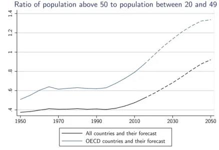
The rapid aging of the population of both developed economies and much of the rest of the world, depicted in Figure 1, is seen as one of the most dangerous economic ills of the next several decades. An increasingly popular thesis, building on Alvin Hansen’s famous 1938 presidential address to the AEA, views developed economies as being afflicted by “secular stagnation,” partly because an aging population creates an excess of savings relative to investments (Alvin Hansen, 1939, Lawrence Summers, 2013, and the essays in Coen Teulings and Richard Baldwin, 2014). A different but related challenge is emphasized by Robert Gordon (2016), who identifies demographic change as the first “headwind” slowing down economic growth in the developed world, for an older population will reduce labor force participation and productivity (workers’ earnings, and presumably productivity, peak in their 40s, e.g., Kevin M. Murphy and Finis Welch, 1990).

.4 .6 .8 1 1.2 1.4 1950 1970 1990 2010 2030 2050

All countries and their forecast OECD countries and their forecast

Ratio of population above 50 to population between 20 and 49

Figure 1: Aging from 1950 to 2015 and projections until 2050 (from the UN data). Aging is measured by the ratio of the population above 50 years old to the population between 20 and 49.

Though both perspectives imply that countries undergoing faster aging should be suffering more from these economic problems,1 _{we show that since the early 1990s or 2000s, the periods commonly}

viewed as the beginning of the adverse effects of aging in much of the advanced world, there is no negative association between aging and lower GDP per capita.2 Figure 2 provides a glimpse of the 1_{Three qualifications to this conclusion should be noted. First, there are non-demographic factors, such as increased}

levels of inequality and slower technological progress, that have also been suggested as potential causes of demand-side secular stagnation. Second, this type of secular stagnation could be partially offset by monetary policy. Third, with international capital flows, aging in one country might affect GDP per capita in others as well.

2_{Thomas Lindh and Bo Malmberg (1999) and James Feyrer (2007) investigate the relationship between}

demo-graphics and aggregate productivity or growth, focusing on pre-1990 data. Both papers find some evidence supporting the notion that the fraction of the population above 50 contributes negatively to GDP per capita. Their findings motivate our baseline choice of demographic variable as the ratio of the population above 50 to those between the ages of 20 and 49.

(3)

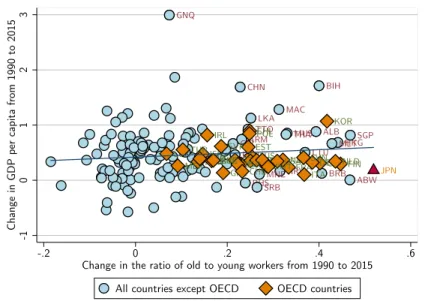
relevant pattern by depicting the raw correlation between the change in GDP per capita between 1990 and 2015 and the change in the ratio of the population above 50 to the population between the ages of 20 and 49. In the next section, we show that even when we control for initial GDP per capita, initial demographic composition and differential trends by region, there is no evidence of a negative relationship between aging and GDP per capita; on the contrary, the relationship is significantly positive in many specifications.

ALB ARM ABW BHS BRB BIH BGR CHN CRI HRV GNQ HKG LTU MAC MLT MUS MNE SRB SGP LKA MKD THA TTO AUS AUT BEL CAN CHL CZE DNK EST FIN FRA DEU GRC HUN ISL IRL ISR ITA LVA LUX

MEXNOR USANZL NLD POL PRT KOR SVK SVN ESP SWE CHE TUR GBR JPN -1 0 1 2 3

Change in GDP per capita from 1990 to 2015

-.2 0 .2 .4 .6

Change in the ratio of old to young workers from 1990 to 2015

All countries except OECD OECD countries

Figure 2: Correlation between aging and growth in GDP per capita (in constant dollars). Aging is defined as the change in the ratio of the population above 50 years old to the population between 20 and 49. GDP per capita data from the Penn World Tables.

The lack of a strong negative association between changes in age structure and changes in GDP per capita is surprising. So what explains it?

The post-1990 era coincides with the arrival of a range of labor-replacing technologies, most recently robotics and artificial intelligence, which provide a wide variety of options for firms to automate the production process. In Section II, we show that countries undergoing more rapid demographic change are more likely to adopt robots (see also Acemoglu and Restrepo, 2017).3 In Section III, we show that when capital is sufficiently abundant, a shortage of younger and middle-aged workers can trigger so much more adoption of new automation technologies that the negative effects of labor scarcity could be completely neutralized or even reversed.

3_{The recent working paper by Nicole Maestas, Kathleen J. Mullen and David Powell (2016) shows a negative}

association between aging and economic growth across US states. To the extent that US states have more similar technologies and more coordinated adoption decisions than countries, the countervailing effects of technology adoption we emphasize would be absent or much muted in this sample.

(4)

I. Aging and GDP Per Capita: The Cross-Country Evidence

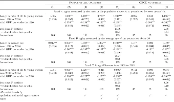
In this section, we start by showing that the relationship depicted in Figure 2 is robust. We use data on GDP per capita from the Penn World Tables and population by age from the United Nations. Our main results are shown in Table 1, which presents regressions of the change in (log) GDP per capita from 1990 to 2015 on our baseline measure of population aging, the change in the ratio of the population above 50 to those between the ages of 20 and 49. Our baseline sample includes 169 countries for which we have data. Panel A reports OLS regressions in changes (long differences) with robust standard errors. Column 1 shows the raw correlation, already depicted in Figure 2. We see a positive but insignificant relationship. The rest of the table investigates the robustness of this relationship.

Table 1: Estimates of the impact of aging on GDP per capita from 1990 to 2015 and from 2000 to 2015.

Sample of all countries OECD countries

(1) (2) (3) (4) (5) (6) (7) (8)

Panel A. aging measured by the ratio of the population above 50 to population between 20 and 49.

Change in ratio of old to young workers 0.335 1.036∗∗∗ _1.162∗∗∗ _0.773∗∗ _1.703∗∗∗ _-0.262 _0.042 _1.186∗∗∗

(from 1990 to 2015) (0.210) (0.257) (0.276) (0.322) (0.411) (0.352) (0.346) (0.458)

Initial GDP per worker in 1990 -0.153∗∗∗ _-0.138∗∗∗ _-0.156∗∗∗ _-0.190∗∗∗ _-0.205∗∗∗ _-0.260∗∗∗

(0.039) (0.042) (0.046) (0.045) (0.072) (0.092)

First-stage F statistic 19.36 7.38

Overidentification test p-value 0.51 0.44

Observations 169 169 169 169 169 35 35 35

Panel B. aging measured by the average age of the population above 20.

Change in average age 0.042∗∗∗

0.090∗∗∗ 0.092∗∗∗ 0.065∗∗∗ 0.103∗∗∗ 0.017 0.001 0.059∗ (from 1990 to 2015) (0.015) (0.017) (0.018) (0.024) (0.023) (0.046) (0.034) (0.035)

Initial GDP per worker in 1990 -0.167∗∗∗ _-0.157∗∗∗ _-0.167∗∗∗ _-0.188∗∗∗ _-0.193∗∗ _-0.187∗∗

(0.038) (0.045) (0.048) (0.046) (0.079) (0.089)

Observations 169 169 169 169 169 35 35 35

Panel C. Long differences from 2000 to 2015

Change in ratio of old to young workers 0.051 0.950∗∗∗ _1.028∗∗∗ _0.215 _0.809∗ _-0.151 _0.009 _0.373

(from 2000 to 2015) (0.210) (0.238) (0.282) (0.259) (0.453) (0.294) (0.285) (0.463)

Initial GDP per worker in 2000 -0.136∗∗∗ _-0.127∗∗∗ _-0.077∗∗ _-0.095∗∗ _-0.259∗∗∗ _-0.256∗∗∗

(0.022) (0.024) (0.031) (0.037) (0.057) (0.054)

Observations 169 169 169 169 169 35 35 35

Differential trends by:

Population and initial age structure X X X X X

Region X X

Notes:The table presents long-difference estimates of the impact of aging on GDP per capita in constant dollars from the Penn World Tables for all countries (columns 1 to 5) and OECD countries (columns 6 to 8). Panels A and C define aging as the change in the ratio of the population above 50 to the population between 20 and 49. Panel B defines aging as the change in the average age of the population above 20. Panels A and B present results for the long differences between 1990 and 2015; while panel C presents results for the long differences between 2000 and 2015. Columns 5 and 8 present IV estimates in which we instrument aging using the birthrate in 1960, 1965, . . . , 1980. The bottom rows indicate additional controls included in the models but not reported. The population and age structure controls include the log of the population and the initial value of our aging measure. We report standard errors robust to heteroskedasticity in parentheses.

Column 2 includes initial log GDP per capita on the right-hand side, while column 3 also adds the initial demographic composition (the ratio of the population above 50 to those between 20

(5)

and 49 and log population in 1990). Column 4 in addition includes a set of dummies for World Bank “regions” (which are Latin America, East Asia, South Asia, Africa, North Africa and Middle East, Eastern Europe and Central Asia, and Developed Countries), thus allowing for differential regional trends. With these controls, the relationship between aging and GDP per capita becomes less positive but remains statistically significant at 5 percent. For example, in column 4, the coefficient estimate is 0.773 (standard error = 0.322).4 Column 5 estimates the same relationship using birthrates for the 1960, 1965, 1970, 1975 and 1980 cohorts as instruments for our demographic change variable, thus purging it from variation due to migration or changing mortality, which could be endogenous to changes in GDP per capita. In this case, the coefficient of interest becomes even more positive and significant, 1.703 (standard error = 0.411).

Columns 6-8 report the same regressions for 35 OECD countries. In this case the OLS estimates are imprecise, though the IV estimates are once again positive and similar to those in the whole sample—1.186 (standard error = 0.458).

Panel B shows similar patterns with a different measure of aging—change in the average age of the population above 20. Panel C shows that the broad picture is also similar when we focus on the post-2000 sample (2000-2015), where concerns about secular stagnation have become more prominent.

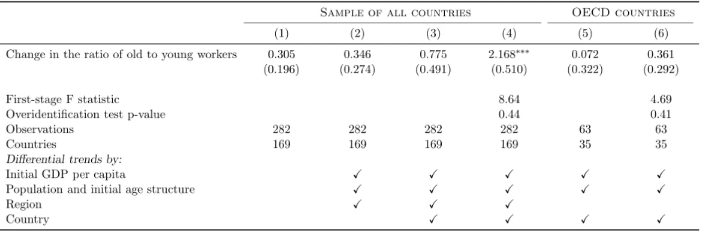
Table 2 extends the sample to 1965 and reports regressions with two differences of 25 years for each country stacked together. Columns 1 and 2 mimic columns 1 and 3 from Table 1 and present very similar results. In addition, columns 3-6 include country dummies, which are equivalent to country-specific linear trends in levels, and report OLS and IV estimates of this more demanding specification. The estimates again point to a positive and statistically significant relationship be-tween population aging and economic growth in the full sample (and a less positive and insignificant one in the OECD).

II. Aging and Robots

Why is there not a strong negative relationship between aging and GDP per capita as predicted by a range of theories, including recent ones on secular stagnation? One possible answer is that technology adjusts so as to undo this potential negative effect. We argue that this answer is 4_{Figure 2 shows that Equatorial Guinea is an outlier, but leaving it out has essentially no impact on the regressions}

reported here. For example, in the equivalent specification to column 4 without Equatorial Guinea, the coefficient estimate is 0.615 (standard error = 0.290). Equatorial Guinea is an oil producer, and we also confirmed that this has no effect on our results by including the share of oil revenues in GDP in 1990 (from the World Bank) as an additional control.

(6)

Table 2: Estimates of the impact of aging on GDP per capita from 1965 to 1990 and 1990 to 2015.

Sample of all countries OECD countries

(1) (2) (3) (4) (5) (6)

Change in the ratio of old to young workers 0.305 0.346 0.775 2.168∗∗∗ _0.072 _0.361

(0.196) (0.274) (0.491) (0.510) (0.322) (0.292)

Observations 282 282 282 282 63 63

Countries 169 169 169 169 35 35

Differential trends by:

Initial GDP per capita X X X X X

Population and initial age structure X X X X X

Region X X X

Country X X X X

Notes:The table presents stacked-difference estimates of the impact of aging on GDP per capita in constant dollars from the Penn World Tables for all countries (columns 1 to 4) and OECD countries (columns 5 to 6). We define aging as the change in the ratio of the population above 50 to the population between 20 and 49. We report estimates for the periods from 1965 to 1990 and 1990 to 2015. Columns 4 and 6 present IV estimates in which we instrument aging using the birthrate in 1960, 1965, . . . , 1980. The bottom rows indicate additional controls included in the models but not reported. The population and age structure controls include the log of the population and the initial value of our aging measure. We report standard errors robust to heteroskedasticity and serial correlation within countries in parentheses.

plausible in two steps. First, in this section, we draw on Acemoglu and Restrepo (2017) to show that countries experiencing more rapid aging are the ones that have been at the forefront of the adoption of one important type of automation technology: industrial robots.

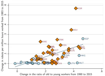
The relationship between aging and adoption of robotics technology is established in Acemoglu and Restrepo (2017) using data from the International Federation of Robotics (IFR), which provides information on industrial robots across a range of industries for 49 countries. We use the same data in the next figure to show the basic cross-country pattern, which reveals a strong correlation between the same measure of demographic change used in our analysis so far—the change in the ratio of the population above 50 to those between 20 and 49, and the change in the number of robots (per million of labor hours) between the early 1990s and 2015.5

Acemoglu and Restrepo (2017) document that this cross-country pattern is robust; it holds if we exclude Korea (a clear outlier) and it holds within the OECD countries. Crucially, as would be expected from a simple model of directed technological change, we also show that it is more pro-nounced in industries that employ younger workers and those in which there are more opportunities for automation.

5_{This figure excludes Japan, since the IRF notes that Japanese data are not comparable over time because of a}

(7)

ARG BRA_BGR COL

HKG

IDNIND LTU MLT

MYS PER PHL PAK ROM SGP THA VEN VNM AUT AUS BEL CHE CZE DEU DNK EST ESP FIN FRA GRC HUN ISL IRL ISR ITA KOR LVA USA NLD NOR NZL POL PRT CHL SWE SVK SVN TUR GBR 0 .1 .2 .3 .4 .5 .6

Change in robots per million hours worked from 1993 to 2015 ₀ _.2 _.4 _.6

Change in the ratio of old to young workers from 1990 to 2015

Figure 3: Correlation between change in the ratio of old to young workers between 1990 and 2015 and change in robots per million hours worked between 1993 and 2014 (from the International Robotics Federation).

III. Can Labor Scarcity Lead to Higher GDP Per Capita?

In this section, we undertake the second, theoretical step in our argument. Drawing on Acemoglu (2010) and Acemoglu and Restrepo (2016), we demonstrate that the scarcity of younger and middle-age labor can trigger sufficient adoption of robots (and other automation technologies) so as to actually increase aggregate output, despite the reduced labor input.

For illustration purposes, we use a static model. Suppose that the aggregate production tech-nology is given by the following Cobb-Douglas aggregate over the services of a range of tasks,

ln Y = Z 1

0

ln y(i)di. (1)

Each task i can be produced with capital or labor combined with their specialized intermediates, q(i). In particular, as in Acemoglu and Restrepo (2016), we assume that tasks i ≤ θ are automated and can be produced using capital or labor, with the production function

y(i) = q(i)η(k(i) + l(i))1−η. (2)

Tasks i > θ can only be produced using labor, and their production function takes the form

y(i) = q(i)ηl(i)1−η, (3)

where η ∈ (0, 1). Intermediates, the q(i)’s, can be produced at the marginal cost of one unit of the final good, and are supplied by a monopolist which charges a constant markup of χ ∈ (0, 1).

(8)

The monopolist also chooses θ ∈ [0, 1] at cost C(θ)Y , which is interpreted as a (domestic) tech-nology choice to adapt robotics or other automation techniques to the conditions of the country in question. We assume that C is twice differentiable, strictly increasing (reflecting the fact that au-tomating more tasks is costly for the monopolist), strictly convex (with a positive second derivative everywhere), and satisfies the Inada condition limθ→1C′(θ) = ∞.

We assume that capital and labor are inelastically supplied, with supplies given, respectively, as K and L, and

K > L. (4)

This implies that capital is abundant and cheap relative to labor, which is plausible given the very low interest rates around the world at the moment. This assumption ensures that automating tasks will be profitable and increase aggregate output. In mapping the model to data, we think of L as the supply of younger and middle-aged workers, so that population aging will correspond to a reduction in L—a phenomenon to which we also refer to as an increase in labor scarcity.

Following the same steps as in Acemoglu and Restrepo (2016), equilibrium aggregate output can be expressed as Y = KθL1−θ. Then the profit maximization problem of the monopolist is

max

θ∈[0,1]K

θ_L1−θ_Γ(θ),

where Γ(θ) = ηχ − C(θ) is strictly decreasing, has a negative second derivative everywhere, and satisfies limθ→1Γ′(θ) = 0. The presence of the term ηχ reflects the profits of the monopolist from

the markup on the intermediates.

The profit maximization of the monopolist, combined with the Inada condition on C, implies

ln K − ln L + Γ′

(θ) = 0.

Differentiating this relationship yields

dθ d ln L =

1

Γ′′_(θ) < 0,

since Γ has a negative second derivative. This establishes that labor scarcity—i.e., a lower L— encourages further automation as in Acemoglu (2010) and Acemoglu and Restrepo (2016).

What is the effect of labor scarcity on aggregate output? To answer this question, let us totally differentiate the expression for ln Y , taking into account the indirect effect of ln L working through

(9)

additional automation: d ln Y d ln L = 1 − θ + ∂ ln Y ∂θ dθ d ln L (5) = 1 − θ + ln K − ln L Γ′′_(θ) = 1 − θ − θ εΓ ,

where εΓ= Γ′′(θ)θ/Γ′(θ) > 0 is the elasticity of the derivative of the Γ function.

In view of condition (4), the second term is negative. Thus a lower L creates a direct effect which is to decrease GDP because of the reduction in the labor input, but also a positive effect through additional automation. If the second term, which is negative, is sufficiently large, then the scarcity of labor caused by an aging population can increase GDP. This will be the case if the gap between K and L is sufficiently large (from the second line of (5)), making capital much cheaper than labor, or if the elasticity εΓ is small (from the third line). Hence, the aging of the labor force,

which reduces the available supply of workers to perform productive tasks in the economy, need not reduce GDP per capita, and may in fact increase it, once we take the response of technology into account.

IV. Conclusion

This paper establishes that, contrary to a range of theories including recent ones on demographics-based secular stagnation, there is no negative relationship between between population aging and slower growth of GDP per capita. This is a major puzzle for several theories that have become very popular over the last several years.

One possible explanation for this pattern is the endogenous response of technology—in partic-ular, the adoption of technologies performing tasks previously undertaken by labor. We document that countries undergoing more rapid population aging have adopted more robots, although we do recognize that this evidence is neither causal nor does it establish that the adoption of robots is the mechanism that neutralizes the potential negative effects of population aging on economic growth. We also demonstrate that models of directed technological change can account for the lack of such a negative relationship, and could generate a positive relationship, between population aging and economic growth.

There is a clear need for future work that systematically investigates the relationship between demographic change and GDP growth as well as the channels via which this relationship works.

(10)

References

Acemoglu, Daron and Pascual Restrepo (2016) “The Race between Machine and Man: Implications of Technology for Growth, Factor Shares and Employment” NBER Working Paper No. 22252.

Acemoglu, Daron and Pascual Restrepo (2017) “Demographics and Robots: Theory and Evi-dence” work in progress.

Feyrer, James (2007) “Demographics and Productivity” Review of Economics and Statistics, 89(1), 100-109.

Gordon, Robert (2016) The Rise and Fall of American Growth, Princeton University Press, Princeton New Jersey.

Hansen, Alvin (1938) “Economic Progress and the Declining Population Growth” American

Economic Review, 29(1), 1-15.

Lindh, Thomas and Bo Malmberg (1999) “Age Structure Effects and Growth in the OECD, 1950-1990” Journal of Population Economics, 12(3), 431-449.

Maestas, Nicole, Kathleen J. Mullen and David Powell (2016) “The Effect of Population Aging on Economic Growth, the Labor Force and Productivity” NBER Working Paper No. 22452.

Murphy, Kevin M. and Finis Welch (1990) “Empirical Age-Earnings Profiles” Journal of Labor

Economics, H(2), 202-229.

Summers, Lawrence (2013) “Why Stagnation Might Prove to Be the New Normal” The

Finan-cial Times.

Teulings, Coen and Richard Baldwin (2014) Secular Stagnation: Facts, Causes and Cures, CEPR Press.