Dissolution of Cavities and Porous Media: a Multi-Scale View

Granada (Spain), April 22-25, 2013

Dissolution of Cavities and Porous Media: a

Multi-Scale View

Michel Quintard1,2

1_{Universit´e de Toulouse ; INPT, UPS ; IMFT (Institut de M´ecanique des} Fluides de Toulouse) ;

All´ee Camille Soula, F-31400 Toulouse, France quintard@imft.fr

2_{CNRS ; IMFT ;} F-31400 Toulouse, France

Keywords:Dissolution, Cavity, Porous Media, Non-Equilibrium Models, Wormhol-ing, Effective Surface.

Abstract. Dissolution of underground cavities or porous media involves many

different scales that must be taken into account in modeling attempts. This paper presents a review of some of these problems. The paper starts with an introduction to non-equilibrium models, which play an important role in understanding dissolution physics for such media. In particular, their funda-mental importance in catching dissolution instability diagrams is emphasized. A second multi-scale aspect is the introduction of the concept of effective sur-face for dealing with heterogeneous and/or rough sursur-faces. All these concepts may be used to develop efficient large-scale simulations. Examples are given for simple situations which emphasize the strong coupling between dissolution and buoyancy plumes generated within the dissolution boundary layer.

1 Introduction

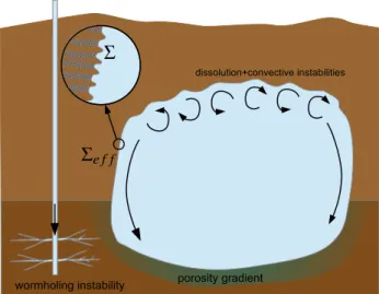
Dissolution of underground cavities are found in many fields such as min-ing of saline formations, karst formation, etc [7, 26]. While dissolution mecha-nisms are not restricted to natural media, the multiple-scale aspects associated with dissolution are inherent to any geological application. This multiple-scale feature is illustrated in Figure 1 which, in a very schematic manner, presents several aspects associated to the injection of a dissolving fluid in a geologi-cal formation (acid injection in petroleum engineering, solution mining, ...) or dissolution through natural water circulation. Typically, one may have the dis-solution of a porous medium, which under certain circumstances may lead to a dissolved region with a porosity gradient before a true fluid cavity, or an imper-vious rock formation with a more direct route to a fluid cavity. Various types of heterogeneity will make the multi-scale feature more complicated. Pore-scale modeling is inaccessible to direct modeling at the cavity Pore-scale, and some sort of macro-scale modeling is necessary. Macro-scale models are not neces-sarily unique, as will be discussed in the next section (discussion about local equilibrium or local non-equilibrium models). Similarly, in the case of a solid rock formation with a sharp dissolving interface, it is often difficult to take into account in a direct manner at the cavity-scale small-scale heterogeneities and/or roughness over the interface. The macro-scale model takes often the form of an effective surface theory, and this point will be discussed later in this paper. Finally, additional intermediate scale features are process dependent, especially the structures induced by dissolution instabilities (wormholing) or coupling between dissolution and hydrodynamic instabilities (notably natural convection and salt fingering). These latter aspects will be discussed in the last section.

2 Porous Media Models

In this section, we discuss the introduction of macro-scale models in a sim-ple case to illustrate the discussion. Suppose the liquid phase, denoted β, is a binary mixture containing species A and B and the solid phase σ contains only species A. The balance equations may be written

∂ρβ

∂t +∇ · (ρβvβ) = 0 (1)

∂ (ρβωAβ)

Figure 1: Cavity dissolution: an illustration of various multi-scale problems

where ωAβ represents the mass fraction of species A and a similar equation

hold for species B. The mass balance equation for the σ-phase is written as

∂ρσ

∂t +∇ · (ρσvσ) = 0 (3)

Of course, the problem must be completed by momentum and energy balances. It is often assumed a quasi-steady coupling between the dissolution problem and the other transport problems (i.e., velocity is assumed to be a known field and temperature is nearly uniform over the averaging volume). At the β− σ interface (denoted by Aβσ in the following text), the chemical potentials for

each species should be equal between the different phases and this results in a classical equilibrium condition

ωAβ= ωAeq at Aβσ (4)

The mass balance for species A at the β− σ interface gives

ρβωAβ(vAβ− w) · nβσ = ρσωAσ(vAσ− w) · nβσ at Aβσ (5)

where

ρβωAβvAβ= ρβωAβvβ− ρβDAβ∇ωAβ (6)

The total mass balance at the β− σ interface gives

where w represents the velocity of the interface. As ωBσ = 0 in the solid

phase, we may write

ρβωAβ(vAβ− w) · nβσ= ρβ(vβ− w) · nβσ at Aβσ (8)

We have now all in hands to discuss the development of macro-scale models. Pore-scale modeling of dissolution processes [3] shows how complex is the interaction between the various transport processes. In particular, the interface evolution may be very complex and process dependent [19]. One is not sur-prised that the development of macro-scale models is therefore very difficult. Indeed, one may consider that this is still an open problem, if one considers the historical aspects and complex interactions previously mentioned. Even if one consider a quasi-steady coupling, the problem of active dispersion (disper-sion with mass exchange at the interface) is known to lead to various models. In particular, we may develop two classes of model if one looks at the dif-ference between the equilibrium concentration and the average concentration. If this difference is very small, the situation is called local equilibrium, and our simple case leads to a very straightforward macro-scale equation for the concentration

ΩAβ= ωAeq (9)

where ΩAβ is the intrinsic average mass fraction. The non-equilibrium case

may lead to various models, since the exchange may feature non-local in space and time mechanisms. At first order, one may follow the works of [21, 22, 14, 6, 23] to derive a general dissolution equation under the form of

∂εβρβΩAβ ∂t +∇·(εβρβΩAβUβ+ ...) =∇· ( εβρβD∗Aβ· ∇ΩAβ ) +Kβσ (10)

where εβ is the fluid volume fraction, Uβ the interstitial velocity, D∗Aβ the

active effective dispersion tensor, and Kβσthe mass exchange term. It is often

approximated as

Kβσ=−α (ΩAβ− ωAeq) + ... (11)

The dots in these equations account for additional terms that may be gen-erally written under the form of additional convective terms, thus potentially affecting the front velocity. It is important to acknowledge that, if these terms cannot be neglected, the traditional expression Kβσ=−α (ΩAβ− ωAeq) does

not account for all the exchange flux! This has been recognized in some cases, as illustrated in [13]. Another feature that is often ignored by “common” knowledge is that the active dispersion tensor, D∗_Aβ, is not necessarily equal to the passive one (i.e., the one with no-flux at Aβσ, see for instance illustration

How does the various models affect the macro-scale behavior? One ex-ample is illustrated in Figure 2. This figure represents the dissolution patterns obtained by injection of a dissolving fluid into a homogeneous porous medium. The pictures represent the porosity field (blue=initial porosity, red=dissolved area, i.e., pure fluid) for various injection flow-rates. The curve is the ratio of the injected volume at breakthrough versus the pore volume. The first picture represents a case of local equilibrium dissolution (characterized by a thin dis-solution front). The process is stable at low velocity. Increasing the velocity leads to the development of well known unstable dissolution fronts [15, 8, 9, 14]. Increasing the velocity also triggers the appearance of non-equilibrium dissolution regimes, starting with the ramified wormholing regime. These regimes are characterized by thick dissolution fronts over which porosity varies continuously. It is very interesting to find that the dissolution front may be sta-ble again at very high velocity, because of the non-equilibrium mechanisms.

The dominant wormhole regime is used in petroleum engineering to bypass low permeability areas near well-bores. How to find the optimal conditions? It was shown in [14] that the optimal condition is found at the junction between the dominant wormhole, local equilibrium dissolution pattern and the ramified wormhole, local equilibrium pattern. This illustrates the interest of non-equilibrium models for describing dissolution processes. Another interest of non-equilibrium dissolution models is the fact that their represent a diffuse in-terface model for dissolution and can be used to model fluid/solid cavity disso-lution problems as illustrated and discussed in [18], without explicit treatment of the interface.

3 Effective Surface modeling

Another interesting multi-scale aspect associated to dissolution problem is the fact that, often, the dissolving surface is heterogeneous as it is illustrated in Figure 3.

The top drawings in this figure represent the dissolution history of the ac-tual surface of a stratified medium, subjected to a chemical reaction with a first order reaction rate which depends on the material. Generally, depend-ing on the Damkh¨oler numbers, the receddepend-ing surface velocity variations create roughnesses. For some boundary conditions for the large-scale problems, the surface roughness becomes quasi-steady and the receding velocity becomes a constant. This receding velocity depends on the roughnesses and the flow con-ditions [25]. One understands that catching this local behavior requires solving the transport equations at this scale, which is in general orders of magnitude lower than the process scale (cavity, well, ...). Therefore, it is interesting to

Figure 2: Diagram of dissolution patterns for injection of a dissolving fluid in a porous medium (after [5] work)

͢

t ∞

t>0

t=0

Figure 3: Real surface dissolution history and the illustration of the concept of effec-tive surface.

W

W

W

...

...

x

y

S

L

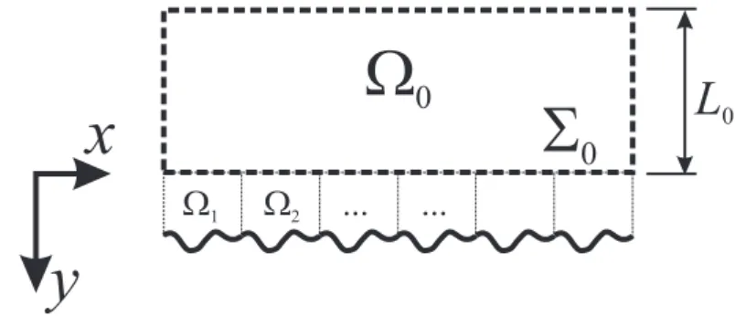
Figure 4: The domain decomposition method

investigate the possibility of replacing this heterogeneous, rough surface by a smooth, homogenous effective surface. The equivalence criterion is essentially the obtainment of the same receding velocity. Given the transient nature of the dissolution of such heterogeneous, rough surfaces, several questions must be solved:

• where to put the surface,

• which effective boundary condition to apply at the effective surface?

The case without dissolution has received a lot of attention especially for the case of Navier-Stokes equations over the rough surface [1, 2, 20, 24, 17]. The technique to derive effective surface and boundary conditions is generally based on a decomposition method, as illustrated in Fig. 4, with a bulk volume where the original equations are solved and unit-cell small regions over the surface where the solution of the transport equations is sought under the form of a deviation to a n-th order continuation of the bulk solution. In the case of Navier-Stokes equations, for an arbitrary position of the effective surface, the effective surface boundary condition has the form of a Navier condition. Using Taylor’s expansion one can change easily the position of the effective surface, which will also change the effective surface boundary condition. For the Navier-Stokes equations, it is possible to determine the position at which the Navier condition reverts to the no-slip condition.

Figure 5 illustrates the concept of effective surface. The top drawing rep-resents the actual problem, here the development of a boundary layer over a rough surface. The bottom figure represents the effective surface treatment, with the effective surface positioned at the place which gives the no-slip con-dition.

For a reactive surface, without dissolution, it was found that, for a given po-sition of the effective surface, the effective boundary condition is a first order

Figure 5: Illustration of the concept of effective surface

reaction rate condition, but with an effective reaction rate that depends on the actual reaction rates, the roughnesses and flow conditions, as well as the ef-fective surface position. An example of calculation is plotted Figure 6, which represents the ratio of the effective reaction rate over the surface average of the point reaction rate, versus the mean value of the surface Damkh¨oler number, for various unit cell geometry. For small Damkh¨oler numbers, the effective reaction rate is equal to the surface average, kavdefined by the surface integral

of k over the surface divided by the projected surface. This can be explained by the fact that, in this case, the concentration near the surface is almost con-stant, thus giving a flux proportional to the point reaction rate. This ratio tends to decrease with increasing Damkh¨oler numbers. For very large Damkh¨oler numbers, the concentration is almost zero along the surface. Kef f becomes a

constant, which is equal to the surface harmonic average in the case of a flat surface, denoted kh.

The picture becomes a little bit more complicated if one takes into account the surface evolution with dissolution [25]. If we start with a flat surface:

• the initial effective reaction rate will be the surface arithmetic average, • after a transient evolution, the surface recession velocity becomes a

con-stant with an effective reaction rate equal to the maximum point reaction rate. In fact, the surface roughness adapts to the heterogeneity with a re-cession velocity determined by the weakest (i.e., the highest reaction rate) material. The ratio of the reaction rates will determine the rough-ness itself, but not the recession velocity!

Figure 6: Effective reaction rate as a function of the Damkh¨oler number (from[24])

flat and the effective reaction rate is equal to kh. For intermediate cases, the

roughness evolution and the associated effective reaction rate is complex and, so far, must be determined experimentally or numerically.

4 Dissolution Structures

At this point, length-scales have been determined initially by the material and domain properties. When studying the concept of effective surface, we already have seen that the surface roughness, while staying of the same order as the original heterogeneity, becomes process dependent. This is such that no a priori effective surface theory may be used without computing the surface geometry evolution. The introduction of process dependent scales in the anal-ysis is often required when considering the existence of instabilities. In this section, we will consider two types of instabilities:

• Dissolution instabilities: the dissolution process is at the core of the

instability onset,

• Coupling between classical hydrodynamic instabilities such as

convec-tive patterns and dissolution.

The impact of dissolution instabilities has been the object of discussion in Sec. 2. Figure 2 shows that small scales can be created through the development of dissolution instabilities, and this is still an open problem to develop effi-cient numerical methods to obtain the wormholing dynamic for domains of

Figure 7: Dissolution of a tube for various P´eclet and Rayleigh numbers (from [18])

industrial scales. Attempts have been made to develop averaged models incor-porating the wormhole dynamics, or other instability patterns, and we refer the reader to some literature on the subject to understand the different estimates and possibilities that have been explored [11, 12, 4].

Coupling with hydrodynamic instabilities is another complex, and still open, problem. While coupling with inertial flow vortices is also a very important question, a typical hydrodynamic instability that often plays a very important role is natural convection arising from density variations with concentration. This is quite inevitable and typical for salt cavities [10]. Figure 7 shows the dissolution of a tube for various P´eclet and Rayleigh numbers, as obtained numerically by [18].

The interpretation is the following:

• for small Rayleigh and P´eclet numbers, the concentration gradients are

relatively small within the tube and the concentration field is symmetric. As a consequence, the dissolution is symmetric and the tube wall slope small,

convec-Figure 8: Corium-Concrete interaction, close-up near the surface showing the forma-tion of cup-shaped structures (work of [16])

tive boundary layers tend to develop, the flow remains symmetric but the slope wall become large,

• for small P´eclet numbers, if we increase the Rayleigh number,

natu-ral convection starts to play a role, with convective “rolls” of smaller length-scales as the Rayleigh number increases. The flow becomes non-symmetric, hence the dissolving surface, with, for this particular situa-tion, a relatively flat surface at the bottom and a more rough surface at the top where the “salt fingers” are initiated.

• for large Rayleigh numbers, if we increase the P´eclet number, the

insta-bilities are flushed away, with a tendency to decrease the roughness of the dissolved wall.

Depending on the geometry of the system, the interaction between the hydro-dynamic instabilities and the dissolution process may produce different sur-face patterns. If the sursur-face is initially flat and horizontal, a typical cup-shaped structure is generated, as illustrated in Figure 8, which is taken from the work of [16] who explored the interaction between concrete walls and Corium, in the framework of nuclear reactor severe accident studies.

5 Conclusion

In this paper, the emphasis has been put on the various models that can be developed at the different scales characteristic of dissolution problems, pore-scale to Darcy-pore-scale models, the concept of effective surface, and the con-sequences of these models especially in terms of dissolution instabilities or coupling between dissolution and hydrodynamic instabilities. These latter ef-fects create additional intermediate scales which contribute to the complexity of dissolution problems.

The emphasis has been put here on theoretical aspects. Of course, many other aspects are equally important and have received significant contributions in the past decades: experimental characterization of transport properties or large-scale dissolution patterns, pore-scale tomographic observations, dissolu-tion morphology, etc...

Acknowledgements

This review incorporates the contribution of many PhD students and col-laborators, as well as many supporting institutions or companies. This infor-mation can be collected from the various references cited in this paper.

REFERENCES

[1] Y. Achdou, P. Le Tallec, F. Valentin, and O. Pironneau. Constructing wall laws with domain decomposition or asymptotic expansion tech-niques. Computer Methods in Applied Mechanics and Engineering,

151(1-2):215–232, 1998.

[2] Y. Achdou, O. Pironneau, and F. Valentin. Effective boundary conditions for laminar flows over periodic rough boundaries. Journal of

Computa-tional Physics, 147(1):187–218, 1998.

[3] S. Bekri, J. F. Thovert, and P. M. Adler. Dissolution of porous media.

Chem. Engng Sci., 50:2765–2791, 1995.

[4] C. E. Cohen, D. Ding, M. Quintard, and B. Bazin. A large scale dual-porosity approach to model acid stimulation in carbonated reservoir. In

10th European Conference on the Mathematics of Oil Recovery, ECMOR X, volume paper B038, pages 1–9, Amsterdam, 2006.

[5] C. E. Cohen, D. Ding, M. Quintard, and B. Bazin. From pore scale to wellbore scale: Impact of geometry on wormhole growth in carbonate acidization. Chemical Engineering Science, 63(12):3088–3099, 2008.

[6] F. A. Coutelieris, M. E. Kainourgiakis, A. K. Stubos, E. S. Kikkinides, and Y. C. Yortsos. Multiphase mass transport with partitioning and inter-phase transport in porous media. Chemical Engineering Science, 61(14):4650–4661, 2006.

[7] D.C. Ford and P. Williams. Karst Hydrogeology and Geomorphology. Wiley, 2007.

[8] C. N. Fredd and H. S. Fogler. Influence of transport and reaction on wormhole formation in porous media. AIChE Journal, 44(9):1933–1949, 1998.

[9] C. N. Fredd and H. S. Fogler. Optimum conditions for wormhole forma-tion in carbonate porous media: Influence of transport and reacforma-tion. SPE

Journal, 4(3):196–205, 1999.

[10] D. Gechter, P. Huggenberger, P. Ackerer, and H. N. Waber. Genesis and shape of natural solution cavities within salt deposits. Water Resources

Research, 44(11):1–18, 2008.

[11] F. Golfier, B. Bazin, R. Lenormand, and M. Quintard. Core-scale descrip-tion of porous media dissoludescrip-tion during acid injecdescrip-tion - part i: Theoretical development. Computational and Applied Mathematics, 23(2-3):173– 194, 2004.

[12] F. Golfier, M. Quintard, B. Bazin, and R. Lenormand. Core-scale descrip-tion of porous media dissoludescrip-tion during acid injecdescrip-tion - part ii: Calcula-tion of the effective properties. ComputaCalcula-tional and Applied Mathematics, 25(1):55–78, 2006.

[13] F. Golfier, M. Quintard, and S. Whitaker. Heat and mass transfer in tubes: An analysis using the method of volume averaging. J. Porous Media, 5:169–185, 2002.

[14] F. Golfier, C. Zarcone, B. Bazin, R. Lenormand, D. Lasseux, and M. Quintard. On the ability of a darcy-scale model to capture worm-hole formation during the dissolution of a porous medium. Journal of

Fluid Mechanics, 457:213–254, 2002.

[15] M.L. Hoefner and H. S. Fogler. Pore evolution and channel formation during flow and reaction in porous media. AIChE Journal, 34(1):45–54, 1988.

[16] C. Intro¨ıni. Interaction entre un fluide `a haute temp´erature et un b´eton :

contribution `a la mod´elisation des ´echanges de masse et de chaleur. PhD

thesis, Universit´e de Toulouse, 2010.

[17] C. Intro¨ıni, M. Quintard, and F. Duval. Effective surface modeling for momentum and heat transfer over rough surfaces: Application to a natu-ral convection problem. Int. J. Heat Mass Transfer, 54:3622–3641, 2011. [18] H. Luo, M. Quintard, G. Debenest, and F. Laouafa. Properties of a diffuse interface model based on a porous medium theory for solid–liquid disso-lution problems. Computational Geosciences, 16(4):913–932, 2012. [19] L. Luquot and P. Gouze. Experimental determination of porosity and

permeability changes induced by injection of co2 into carbonate rocks.

Chemical Geology, 265:148–159, 2009.

[20] A. Mikeli´c and V. Devigne. Ecoulement tangentiel sur une surface rugueuse et loi de Navier. Annales Math´ematiques BLAISE PASCAL, 9:313–327, 2002.

[21] M. Quintard and S. Whitaker. Convection, dispersion, and interfacial transport of contaminants: Homogeneous porous media. Advances in

Water resources, 17:221–239, 1994.

[22] M. Quintard and S. Whitaker. Dissolution of an immobile phase during flow in porous media. I/&EC Research, 38(3):833–844, 1999.

[23] C. Soulaine, G. Debenest, and M. Quintard. Upscaling multi-component two-phase flow in porous media with partitioning coefficient. Chem Eng

Sci, 66:6180–6192, 2011.

[24] S. Veran, Y. Aspa, and M. Quintard. Effective boundary conditions for rough reactive walls in laminar boundary layers. International Journal of

Heat and Mass Transfer, 52:3712–3725, 2009.

[25] G. L. Vignoles, Y. Aspa, and M. Quintard. Modelling of carbon-carbon composite ablation in rocket nozzles. Composites Science and

Technol-ogy, 70:1303–1311, 2010.

[26] Jo De Waele, Lukas Plan, and Philippe Audra. Recent developments in surface and subsurface karst geomorphology: An introduction.