Oxygen Diffusion Modeling in Titanium Alloys: New Elements on the Analysis of Microhardness Profiles

OATAO is an open access repository that collects the work of Toulouse

researchers and makes it freely available over the web where possible

Any correspondence concerning this service should be sent

to the repository administrator:

tech-oatao@listes-diff.inp-toulouse.fr

This is an author’s version published in:

http://oatao.univ-toulouse.fr/25605

To cite this version:

Vaché, Nicolas

and Monceau, Daniel

Oxygen Diffusion Modeling in

Titanium Alloys: New Elements on the Analysis of Microhardness Profiles.

(2020) Oxidation of Metals, 93 (1-2). 215-227. ISSN 0030-770X

https://doi.org/10.1007/s11085-020-09956-9

Oxygen Diffusion Modeling in Titanium Alloys: New

Elements on the Analysis of Microhardness Profiles

Nicolas Vaché1  _{· Daniel Monceau}1

Abstract

This study focuses on the diffusion of oxygen in titanium alloys during high-temper-ature oxidation. In particular, the model used to obtain thermokinetic coefficients from microhardness profiles was investigated. A literature review shows that micro-hardness profiles are modeled by a simple error function in the same way as oxygen concentration profiles obtained by microprobe analysis (EPMA). The analysis of lit-erature shows that the hypothesis of a linear relationship between microhardness and oxygen content is not true over the entire oxygen concentration range and that a par-abolic relationship is empirically more accurate. A new modeling equation taking into account this parabolic law is proposed as well as a simplified and easier to use form. The relative error of the diffusion coefficients obtained using the simplified equation was then determined. This new model was applied to the experimental microhardness profile of a Ti-6242s sample oxidized at 625 °C. The resulting oxy-gen diffusion coefficient is in excellent agreement with the one determined from EPMA profile using the classic error function model. Finally, other data from litera-ture were analyzed with the new model to obtain an Arrhenius diagram of oxygen diffusivity in Ti-64 alloy between 550 and 850 °C. This diagram gives thermokinetic coefficients D0=1.1 × 10

−₅

exp(−191 kJ/mol

RT ) that are close to those reported for pure α-Ti in the temperature range 550–850 °C.

Keywords _{Titanium · Oxidation · Oxygen diffusion coefficient · Microhardness} profile · Modeling

* Nicolas Vaché

nicolas.vache@ensiacet.fr

1 _{CIRIMAT, CNRS, INP-ENSIACET, Université de Toulouse, 4 allée Emile Monso,} 31030 Toulouse, France

Introduction

Oxygen is used as an addition element to increase the mechanical properties of titanium alloys. In their review, Yan et  al. [1] reported that Ti–6Al–4V can be alloyed up to 0.35 wt% oxygen in order to increase its maximum tensile strength and yield strength before its elongation at break decreases. But like zirconium alloys, α, near-α and α–β titanium alloys can dissolve a huge amount of oxygen in their crystal lattice (about 33 at.% in the α-phase) [2]. An uncontrolled increase in oxygen content of titanium alloys can occur at very high temperatures during casting (T > 1000  °C) or during prolonged exposure to high temperatures in an oxidizing atmosphere. In the first case, oxygen enrichment leads to the stabiliza-tion of the α-phase during cooling, forming an external and brittle layer known as the “α-case” [3]. On the other hand, the oxidation of titanium at temperatures above 400 °C leads to the simultaneous formation of an oxide layer (TiO₂) and an oxygen diffusion z one ( ODZ). T he l atter i s n ot a ssociated w ith p referential α-phase formation, so it is preferable not to call it α-case. The magnitude of ODZ increases parabolically with time because limited by diffusion in the volume [4], and exponentially with temperature as the diffusion coefficient of oxygen varies according to an Arrhenius law [5–7]. The formation of ODZ is also associated with an evolution of the mechanical properties of titanium alloy parts and, more precisely, causes a decrease in ductility and fatigue life of alloys [8–11]. For these reasons, it is necessary to determine the thermokinetic parameters of oxygen dif-fusion in titanium alloys in order to predict the evolution of ODZ as a function of time and temperature.

The electronic probe microanalyzer (EPMA) is a tool for direct measurement of element content and allows oxygen in titanium alloys to be dissociated from other potential hardening elements (e.g., N, C and H). The use of this technique is relevant and widespread in the study of oxygen diffusion in titanium alloys [12,

13]. In cross section, it is possible to perform measurements close to the oxide/ metal interface thanks to a near-micrometer spatial resolution. However, two main limitations can be mentioned: a correction must be made on the raw values due to the formation of a TiO₂ native film on the sample surface. This surface pollution also requires using a reference before each measurement, which com-plicates the experimental procedure and can make it difficult to obtain a reliable measure under 1 at. %. This lack of sensitivity may lead to an underestimation of the measurement of the diffusion zone thickness (ODZ) from EPMA profiles.

As oxygen hardens titanium, measuring a microhardness profile is an easy and efficient method to obtain information about the diffusion of oxygen in the metal. It is an indirect measure of the oxygen content in the metal, which can vary depending on the presence of other hardening elements. Unlike EPMA, micro-hardness is sensitive to small variations in oxygen content [8, 14]. However, the spatial resolution of this technique is limited by the size of the imprint of the indenter. This size is a function of the applied load which also modifies the value of the microhardness measure [15]. Knoop microhardness differs f rom Vickers microhardness in that it has a reduced imprint size in one direction which allows

for microhardness profiles to be made with improved spatial resolution. It is also possible to modify the size of the imprint by decreasing the applied load, but the dispersion of the measurements is then increased. Using nanoindentation is a solution to further improve spatial resolution, but it implies other limitations on the hardness values such as crystallographic orientation and microstructural effects [16].

The present work focuses on microhardness profile modeling to determine the diffusion coefficient of oxygen in the matrix. First, the relationship between micro-hardness measurement and oxygen content of titanium alloys was studied based on literature results. This relationship was then implemented into the preexisting model using the simple error function so as to propose a new model providing a more accu-rate value of the diffusion coefficient from microhardness profile analysis. Finally, this model was applied to analyze the diffusion of oxygen in a Ti-6242s alloy oxi-dized at 625 °C for 3000 h as well as to produce an Arrhenius diagram of the diffu-sion of oxygen in Ti-64 alloys by analyzing literature results.

Experimental Procedure

Experiments were performed on a commercially available Ti–6Al–2Sn–4Zr–2Mo–Si forging alloy (chemical composition is given in Table 1). Information concerning chemical analyses as well as sample preparation and experimental conditions of oxidation tests can be found in Dupressoire et al. [17] and Vande Put et al. [18]. Microhardness imprints were carried out with a 50-g diamond indent; this weight was chosen to homogenize the effect of the microstructure, but it is small enough to keep a satisfactory spatial resolution. Electron microprobe analyses (EPMA) were realized with a Cameca sx50 microprobe using a voltage of 15 kV and a current of 20 nA.

Modeling of Microhardness Profiles

Considering that the diffusion of oxygen in titanium alloys follows a parabolic kinet-ics, the diffusion profiles obtained by EPMA can be modeled using Eq. (1) which is a solution of Fick’s second law in semi-infinite material, assuming a constant con-centration at the surface and a constant diffusion coefficient over the studied concen-tration range [19]:

Table 1 Chemical composition of the Ti-6242s (wt% and wt. ppm) in as-received condition

Ti wt% Al wt% Sn wt% Zr wt% Mo wt% Si wt. ppm C wt. ppm O wt. ppm N wt. ppm

where C₀ represents the initial concentration of the species in the metal [C₀= C (x,

t = 0)], C_S is the surface concentration [C_S = C (z = 0, t)], and D is the diffusion coef-ficient. D is then determined by adjusting the model and the experimental values using the least-squares method. In the literature, microhardness profile modeling is often carried out according to the same mathematical model but by replacing oxy-gen concentration with microhardness (Eq. 2). This model proposed by Strafford and Towell [20] is based on the work of Rosa et al. who found a linear relationship between microhardness and oxygen content up to 2 wt% in a β-Ti alloy between 932 and 1142 °C [21] and was generalized to α, near-α and α-β alloys for all tempera-tures [22–24].

However, another relationship between microhardness and oxygen content can be found in the literature. It was empirically determined by Brown, Folkman and Schussler after studying 152 batches of titanium sponges [25] and mentioned by Liu and Welsh in their study on the effect of oxygen on the mechanical properties of α- and β-titanium alloys [14] as well as by Leyens and Peters in their edited volume [26].

For all these authors, the microhardness of titanium alloys is best described as a parabolic function of oxygen content, i.e.,

With HVT, the hardness of the oxygen-free material, b a coefficient to be determined for each studied alloy and Cx the atomic oxygen concentration.

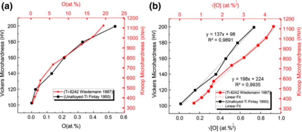
Very few studies dedicated to the relationship between microhardness and oxy-gen content in titanium alloys are available in the literature. To our knowledge, only the studies of Finlay et al. (up to 0.5 at.% of oxygen) [8] and Wiedemann et al. [15] (up to 20  at.% of oxygen) provide experimental microhardness data on unalloyed titanium and Ti-6242 alloy with homogeneous and measured oxygen contents. For each of these data series, microhardness was traced as a function of oxygen con-tent (Fig.  1a) and square root of oxygen content (Fig.  1b). The visualization of these results and the linear regressions in Fig. 1b clearly indicate that the relation-ship between the microhardness of these materials and the oxygen content is bet-ter described using a parabolic law, which is consistent with the empirical law sug-gested by Folkman and the assumption held by Liu & Welsch.

The justification for the parabolic relationship between these two quantities is not immediate and beyond the scope of this work. However, the present study proposes to integrate this law into the model used for microprobe profile analysis (Eq. 1) in order to rewrite the microhardness modeling equation.

(1) C_x−_C 0 C_s−_C 0 =_{1 − erf} � x 2√Dt � (2) �HVx−HV0 � �HV_s−_HV 0 � =1 − erf � x 2√Dt � (3) HVx=HVT+b ∗ √ C_x

According to Eq. 3, the initial hardness HV₀ of an industrial titanium alloy with oxy-gen concentration C₀ is therefore expressed as:

Or,

By combining Eqs. (3) and (4′), the hardness HVx, measured at a distance x from the oxide/metal interface after oxidation, can be expressed as:

The oxygen concentration Cx, measured at a distance x, becomes:

In the same way, the oxygen concentration Cs at the oxide/metal interface, inducing a hardness HVs, can be expressed as:

Equation 1 can therefore be rewritten by replacing Cs and Cx with the two

expres-sions above: (4) HV₀=HV_T+b ∗√C 0 (4′) HVT =HV0−b ∗ √ C₀ (5) HVx=HV0+b ∗ �√ C_x−√_C 0 � (6) C_x= � HV_x−_HV 0 b + √ C₀ �2 (7) C_s= � HV_s−HV 0 b + √ C₀ �2

Fig. 1 Relationship between microhardness and a oxygen atomic percent, b square root of oxygen atomic percent of Ti–cp (data from Finlay 1950) and Ti-6242 (data from Wiedemann et al. [15])

After having developed:

And finally:

Two scenarios are then possible in order to use this equation to model microhard-ness profiles:

Case no. 1: For a given alloy, there exists a former specific study that produced an abacus to convert microhardness measurements into concentration (as in the work of Wiedemann, also used by Shenoy et al. [27] for instance). In this case, hardness values can be converted into concentrations and Eq. 1 can be applied to model the concentration profiles and determine the oxygen diffusion coefficients. This case is the rarest because such a study requires the production of titanium alloys samples with homogeneous oxygen concentration. It is possible to obtain such samples by elaboration or oxidation and homogenization via vacuum treat-ment (as done by Wiedemann). In the absence of a dedicated study, an approxi-mate abacus, for a sample at a given oxidation temperature and time, can be made using microhardness and EPMA profiles. Although a special effort must be made to perform measurements at similar depths, which remains difficult consider-ing the difference between the EPMA interaction pear (1 µm) and the size of the microhardness indent (> 10 µm). But it can be assumed, in view of the influence of oxidation time and temperature on the alloy microstructure that an abacus will have to be made for each [time, temperature] pair.

Case no. 2: The b coefficient is not known, and we wish to estimate the value of the oxygen diffusion coefficient by analyzing hardness profiles. In this case, it is possible to either:

Take an approximate value of b, which, according to the two cases presented here, may vary from 100 to 200 and could also vary depending on the alloys, the type of microhardness measured (Vickers or Knoop) as well as the applied load. Equation 10 can then be used to adjust the experimental microhardness measure-ments to the model, knowing that all terms in the denominator are assumed to be fixed.

Or, to make the assumption that for fairly high microhardness values:

(8) �_HV x−HV0 b +√C0 �2 −_C 0 �_HV s−HV0 b +√C0 �2 −_C 0 =1 − erf � x 2√Dt � (9) �_HV x−HV0 b �2 +₂ � HVx−HV0 b � √C₀+ � √C₀�2−_C 0 � HVs−HV0 b �2 +₂ � HVs−HV0 b � √C₀+ � √C₀�2−_C 0 =1 − erf � x 2√Dt � (10) �HV_x−_HV 0 �2 +2b�HV x−HV0�√C0 �HV_s−_HV 0 �2 +2b�HV s−HV0�√C0 =_{1 − erf} � x 2√Dt �

This assumption allows to simplify Eq. 10 which gives:

Or,

Validity of the Hypothesis

A parametric study of the validity of the assumptions and an evaluation of the relative error between D values from Eqs. 10 and 12 were performed and are pre-sented in Fig. 2 (details on the mathematical development needed for error estima-tion can be found in the “Appendix”). For b values calculated from the literature

�HVx−HV0 �2 ≫2b�HV_x−HV 0�√C0 �HV_s−_HV 0 �2 ≫2b�HV s−HV0�√C0 (11) �HV_x−_HV 0 �2 �HV_s−HV 0 �2 =1 − erf � x 2√Dt � (12) HVx−HV0 HV_s−_HV 0 = � � � �1 − erf � x 2√Dt �

Fig. 2 Relative error between the oxygen diffusion coefficient from the simplified model as compared to the complete model for different values of the b coefficient and of the difference between the meas-ured hardness and the bulk hardness. The fixed parameters are HVs = 980 HV, HV0 = 330 HV and

data (Fig. 1b), the oxygen diffusion coefficients obtained using the simplified model are 30% lower than those obtained using the complete model. The error increases with the value of b and decreases with high hardness values. This result is con-sistent with the approximation made to establish the simplified model, which was (HVi − HV0)2 ≫ 2b(HVi − HV0). The evolution of the ratio between the two

coef-ficients as a function of the difference (HVi − HV0) shows that the fit between the

simplified model and the experimental data is more accurate if the data range is restricted to the highest microhardness values. Actually, the least-squares difference data adjustment method favors small differences for the first experimental points with a high hardness value (thus minimizing more effectively the sum of the dif-ferences). In order to minimize the error, it may still be advantageous to only use experimental results that display a hardness 100–200 HV higher than the bulk hard-ness. From a practical point of view, the first measurement point, if very close to the oxide-metal interface, could also be removed from the adjustment data range because this value is often erroneous due to the proximity of the oxide layer which has a high hardness.

Application 1: Oxidation of Ti‑6242s

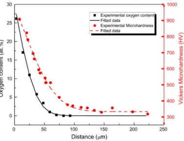
Samples of Ti–6Al–2Sn–4Zr–2Mo–Si were oxidized at 625  °C in air prior to EPMA and microhardness characterization [18]. The oxygen concentration and microhardness profiles as well as the curves representing the adjusted data are shown in Fig. 3. For each series of data, the effective oxygen diffusion coeffi-cient was determined using the simple error function, i.e., Eq. 2 (least-squares

Fig. 3 Oxygen concentration and microhardness profiles of the sample heat treated at 625 °C for 2958 h in air. The experimental values are represented by squares and circles and the fitted values by solid and dash lines

Table 2 Diffusion coefficients of oxygen in Ti-6242 alloy at 625 °C obtained from EPMA and micro­ hardness profiles

Technique Mode! D (m2 _{s-1) HV or [O] surface HV or [O] bulk}

EPMA 1- erf 3.6x 10-17 29.9 at% Oat%

Microhardness 1- erf l.2xJ0-16 980HV 333HV

Microhardness

VI -

fit). The results reported in Table 2 show that two different coefficients are

found for the Ti-6242 s sample depending on the characterization technique used. The oxygen diffusion coefficient calculated from the microhardness profile

( l.2x 10-16 m2 _{s-1) is nearly 3 times higher than the one obtained from EPMA}

(3.6x 10-1_{7 m}2 _ç1_{). The surface and bulk oxygen concentration and microhard­}

ness used in the fitting are also given in Table 2.

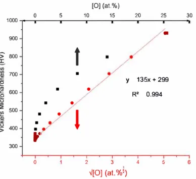
A representation of hardness as a fonction of oxygen concentration (black squares) both modeled by the simple error fonction (Eq. 2) using these two coeffi­ cients is proposed in Fig. 4. For each parameter, a distance step of 10 µm between each point was chosen. It is clear from Fig. 4 that the two quantities are not lin­ early related, but by plotting the hardness as a fonction of the square root of the modeled concentration (red circles in Fig. 4), the parabolic law highlighted in the first part of this work can be found again.

(0) (al.%) 0 5 10 15 20 25 30 1000

•

>

t

_"'

•

•

•

t

JJ

Fig. 4 Modeled microhardness value as a function of modeled oxygen concentration (black squares) and square root of modeled oxygen concentration (red circles) (Color figure online)

The small and simple modification of Eq. 2 leading to Eq. 12 applied to the microhardness data makes it possible to determine a new value for the oxygen diffu-sion coefficient from the microhardness measurements: D = 4.4 × 10−17 _m2 _s−1_{. The}

relative error between the coefficients obtained from EPMA and microhardness pro-files is now below 25%, whereas it was greater than 200% using the classic model based on Eq. 2.

Application 2: Arrhenius Diagram of the Ti‑64 Alloy

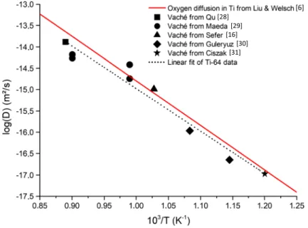
The new model that uses the square root of the error function (Eq. 12) was applied to determine the oxygen diffusion coefficients from microhardness profiles obtained on Ti-64 titanium alloys between 550 and 850 °C found in the literature [16, 28–31]. The resulting data were plotted in an Arrhenius diagram (Fig. 5), and the pre-expo-nential factor, D0, and the activation energy, Q, of the diffusion of oxygen were

obtained:

Calculations lead to D0 = 1 × 10−5 m2 s−1 and Q = 191 kJ mol−1. These values are

close to those found for oxygen diffusion in α-titanium represented by a red line in Fig. 5 [7]. This result confirms that even though the oxygen diffusion coefficient is supposed to be higher in the β-phase of Ti-64 alloys [21], the low solubility of

D = D₀∗_exp ( −_Q R ∗ T ) [28] [29] [16] [30] [31] [6]

Fig. 5 Arrhenius plot of the diffusion coefficients of oxygen in Ti-64 obtained by fitting microhardness profiles from literature using Eq. 12 (in black symbols and linear fit in dots). The diffusion coefficients of oxygen in the α-Ti phase from Ref. [6] are also drawn for comparison purposes (red line) (Color figure online)

oxygen in this phase (8 at.% at 1700 °C [32]) means that diffusion is driven by trans-port in the α-Ti phase. The Arrhenius plots of oxygen diffusivity in each alloy (Ti-64 and α-Ti) are therefore very close.

Conclusion

This paper confirms that an empirical parabolic relationship does exist between microhardness measurements and the oxygen content of oxidized α-titanium alloys. It was then shown that this parabolic relationship could be taken account in the modeling of microhardness profiles by modifying the simple error function. A new model is herein proposed which includes a simplification that generates a rela-tive error of about 25% on the diffusion coefficient. Results using this new model show that the coefficient determined from the square root of the error function is much more accurate than the one determined by a simple error function. Finally, this analytical method was used to produce an Arrhenius diagram of oxygen diffu-sion in Ti-64 alloys from microhardness profiles found in the literature. In addition, the thermokinetic coefficients obtained are very close to those determined for α-Ti alloys.

Acknowledgements The authors gratefully acknowledge the support of Airbus Operations SAS and the fruitful discussions with Benjamin Dod and Yannick Cadoret.

Appendix: Mathematical Development Associated with Fig. 2

The  ratio  between the two oxygen diffusion coefficients can be expressed from Eqs. 10 and 12 [20]. Terms x2 4t can be simplified, D_{simplified model} D_{complete model} = 1 4t ∗ ⎡ ⎢ ⎢ ⎣ x erf−1 � 1−(HVx−HV0) 2 (HVs−HV0)2 � ⎤ ⎥ ⎥ ⎦ 2 1 4t ∗ ⎡ ⎢ ⎢ ⎣ x erf−1 � 1−(HVx−HV0) 2_{+2b(HVx−HV0)√C0} (_HVs−HV0)2+2b(_HVs−HV0)_√C0 � ⎤ ⎥ ⎥ ⎦ 2 D_{simplified model} D_{complete model} = ⎡ ⎢ ⎢ ⎣ 1 erf−1 � 1−(HVx−HV0) 2 (_HVs−HV0)2 � ⎤ ⎥ ⎥ ⎦ 2 ⎡ ⎢ ⎢ ⎣ 1 erf−1 � 1−(HVx−HV0) 2_{+2b(HVx−HV0)√C0} (_HVs−HV0)2+2b(_HVs−HV0)_√C0 � ⎤ ⎥ ⎥ ⎦ 2

Then,

As there is no explicit form of the reciprocal error function erf−1_{(x), the}

approxima-tion of Winitzki was used [33]:

With a ≈ 0.147, the largest relative error of this equation is about 2 × 10−3.

References

1. M. Yan, W. Xu, M. S. Dargusch, H. P. Tang, M. Brandt and M. Qian, Powder Metallurgy 57, 251 (2014).

2. C. E. Shamblen and T. K. Redden, in The Science, Technology and Application of Titanium, eds. R. I. Jaffe and N. E. Promisel (1970), p. 199.

3. K. S. Chan, M. Koike, B. W. Johnson and T. Okabe, Metallurgical and Materials Transactions A 39, 171 (2008).

4. H. Mehrer, H. Bakker, K.-H. Hellwege, H. Landolt, R. Börnstein and O. Madelung (eds.),

Numeri-cal Data and Functional Relationships in Science and Technology, (Springer, Berlin, 1990).

5. D. David, G. Beranger and E. A. Garcia, Journal of the Electrochemical Society 130, 4 (1983). 6. J. Unnam, R. N. Shenoy and R. K. Clark, Oxidation of Metals 26, 231 (1986).

7. Z. Liu and G. Welsch, Metallurgical Transactions A 19, 1121 (1988). 8. W. L. Finlay and J. A. Snyder, JOM 2, 277 (1950).

9. L. Bendersky and A. Rosen, Engineering Fracture Mechanics 20, 303 (1984).

10. R. Gaddam, M.-L. Antti and R. Pederson, Materials Science and Engineering: A 599, 51 (2014). 11. D. P. Satko, et al., Acta Materialia 107, 377 (2016).

12. R. H. Olsen, Metallography 3, 183 (1970).

13. R. Gaddam, B. Sefer, R. Pederson and M.-L. Antti, Materials Characterization 99, 166–174 (2015). 14. Z. Liu and G. Welsch, Metallurgical Transactions A 19, 527 (1998).

15. K. E. Wiedemann, R. N. Shenoy and J. Unnam, Metallurgical Transactions A 18, 1503 (1987). 16. B. Sefer, J. J. Roa, A. Mateo, R. Pederson, and M.-L. Antti, in Proceedings of the 13th World

Con-ference on Titanium, eds. V. Venkatesh, A. L. Pilchak, J. E. Allison, S. Ankem, R. Boyer, J.

Christo-doulou, H. L. Fraser, M. A. Imam, Y. Kosaka, H. J. Rack, A. Chatterjee, and A. Woodfield (Wiley, Hoboken, 2016), p. 1619.

17. C. Dupressoire, A. Rouaix-Vande Put, P. Emile, C. Archambeau-Mirguet, R. Peraldi and D. Mon-ceau, Oxidation of Metals 87, 343 (2017 ).

18. A. Vande Put, C. Thouron, P. Emile, R. Peraldi, B. Dod, and D. Monceau, in Proceedings of the

14th World Conference on Titanium (2019).

19. J. Crank, The Mathematics of Diffusion, 2nd edn. (Clarendon Press, Oxford, 1975). 20. K. N. Strafford and J. M. Towell, Oxidation of Metals 10, 41 (1976).

21. C. J. Rosa, Metallurgical Transactions 1, 2517 (1970).

22. M. Göbel, V. A. C. Haanappel and M. F. Stroosnijder, Oxidation of Metals 55, 137 (2001). 23. S. Zabler, Materials Characterization 62, 1205 (2011).

D_{simplified model} D_{complete model} = � erf−1 � 1 −(HVx−HV0) 2 +2b(HVx−HV0)√C0 (HVs−HV0) 2 +_2b(HVs−HV0)√C0 ��2 � erf−1 � 1 −(HVx−HV0) 2 (HVs−HV0) 2 ��2 erf−1_{(x) ≈} ⎡ ⎢ ⎢ ⎢ ⎣ − 2 𝜋_a − ln�1 − x2� 2 + � � � � � � 2 𝜋_a + ln�1 − x2� 2 �2 −1 aln�1 − x 2� ⎤ ⎥ ⎥ ⎥ ⎦ 1 2

24. J. Baillieux, D. Poquillon and B. Malard, Journal of Applied Crystallography 49, 175 (2016). 25. H. Conrad, Progress in Materials Science 26, 123 (1981).

26. C. Leyens and M. Peters (eds.), Titanium and Titanium Alloys: Fundamentals and Applications, 1st edn. (Wiley, New York, 2003).

27. R. N. Shenoy, J. Unnam and R. K. Clark, Oxidation of Metals 26, 105 (1986). 28. J. Qu, P. J. Blau, J. Y. Howe and H. M. Meyer III, Scripta Materialia 60, 886 (2009). 29. K. Maeda, et al., Journal of Alloys and Compounds 776, 519 (2019).

30. H. Guleryuz and H. Cimenoglu, Journal of Alloys and Compounds 472, 241 (2009).

31. C. Ciszak, I. Popa, J.-M. Brossard, D. Monceau and S. Chevalier, Corrosion Science 110, 91 (2016). 32. H. Okamoto, Journal of Phase Equilibria and Diffusion 32, 473 (2011).

33. S. Winitzki, A Handy Approximation for the Error Function and Its Inverse, A Lecture Note

Obtained Through Private Communication (2008)

Publisher’s Note Springer Nature remains neutral with regard to jurisdictional claims in published maps and institutional affiliations.