Analysis of one month of CHAMP state vector and accelerometer data for the recovery of the gravity potential

HAL Id: hal-00296748

https://hal.archives-ouvertes.fr/hal-00296748

Submitted on 17 Jun 2003

HAL is a multi-disciplinary open access

archive for the deposit and dissemination of

sci-entific research documents, whether they are

pub-lished or not. The documents may come from

teaching and research institutions in France or

abroad, or from public or private research centers.

L’archive ouverte pluridisciplinaire HAL, est

destinée au dépôt et à la diffusion de documents

scientifiques de niveau recherche, publiés ou non,

émanant des établissements d’enseignement et de

recherche français ou étrangers, des laboratoires

publics ou privés.

Analysis of one month of CHAMP state vector and

accelerometer data for the recovery of the gravity

potential

E. Howe, L. Stenseng, C. C. Tscherning

To cite this version:

E. Howe, L. Stenseng, C. C. Tscherning. Analysis of one month of CHAMP state vector and

accelerom-eter data for the recovery of the gravity potential. Advances in Geosciences, European Geosciences

Union, 2003, 1, pp.1-4. �hal-00296748�

c

European Geosciences Union 2003

Advances in

Geosciences

Analysis of one month of CHAMP state vector and accelerometer

data for the recovery of the gravity potential

E. Howe, L. Stenseng, and C. C. Tscherning

Department of Geophysics, University of Copenhagen, Juliane Maries Vej 30, DK-2100 Copenhagen, Denmark

Abstract. The energy conservation method is based on knowledge of the state vector and measurements of non-conservative forces. This is or will be provided by CHAMP, GRACE and GOCE. Here the analysis of one month of CHAMP state vector and accelerometer data is described.

The energy conservation method is used to estimate the gravity potential at satellite altitude. When doing so we con-sider the tidal potential from the sun and the moon, the ex-plicit time variation of the gravity potential in inertial space and loss of energy due to external forces.

Fast Spherical Collocation have been used to estimate a gravity field model to degree and order 90, UCPH2002 04. This gravity field model is compared to EGM96 and

EIGEN-2. The largest differences with respect to EGM96 are

found at those places where the gravity data used to de-termine EGM96 had the largest uncertainty. EIGEN-2 and UCPH2002 04 are similar, though there are some differences in Antarctica and Central Asia.

Key words. CHAMP, energy conservation, gravity field

model, collocation

1 Introduction

The German CHAlleging Minisatellite Payload (CHAMP) was launched in July 2000. It carries a GPS receiver and a three-axes accelerometer. This is the first satellite that pro-vides the user with position and accelerometer measurements for geopotential recovery, enabling the use of the energy con-servation method.

From energy conservation in inertial space the relationship between the gravitational potential and the state vector of the satellite can be derived. The state vector is obtained from the CHAMP Rapid Science Orbit (RSO) product (Michalak et al., 2003). Besides the potential due to the mass of the earth, we have considered the tidal potential from the sun and the moon, loss of energy due to external forces and the

Correspondence to: E. Howe (eva@gfy.ku.dk)

explicit time variation of the gravitational potential in inertial space.

The pre-processed accelerometer data (F¨orste, 2002) were used to estimate the energy loss, however scale error and bias in the accelerometer had to be estimated. A comparison with the high degree and order gravity potential reference field EGM96 (Lemoine et al., 1998) has been used to estimate a scale factor for the along-track accelerometer.

The RSO state vector data (x, y, z, vx, vy, vz) and the

pre-processed accelerometer data (ax, ay, az) from August

2001 have been analysed. The RSO is available as fourteen hour files starting at 10:00 and 22:00. The orbit solution in the beginning and end of a file is poorly constrained in the orbit determination process. We therefore divided the orbit files into twelve hour files starting at 11:00 and 23:00. This minimise the discontinuity of the state vector.

The state vector is given in the Conventional Terrestrial System (CTS) and the accelerometer data is given in a lo-cal instrument reference frame. The x-axis is aligned along the radial direction, the y-axis is along the direction towards the boom (along-track) and the z-axis is completing the triad along the perpendicular direction of the orbital plane (cross-track).

During the investigations of the method it was found that the error of the energy conservation method is sensitive to variations in the solar activity. An analysis of the solar ac-tivity lead us to select August 2001 because of uniform low variability in this period (Bilitza, 2002).

The feasibility of the energy conservation method was ear-lier tested by Gerlach et al. (2003), Howe and Tscherning (2003) and Han et al. (2002). The first two groups made use of the rapid science orbits for a small time period. The first group used a semi-analytical approach to determine the gravity field model to degree and order 60 by a 2D-Fourier method. The third group used precise orbits for a 16-day pe-riod and a numerical procedure to determine a gravity field model to degree and order 50.

In this paper the method of Fast Spherical Collocation based on least squares collocation (Sans´o and Tscherning,

2 E. Howe et al.: Analysis of one month of CHAMP state vector and accelerometer data 2002) is used to determine a gravity field model to degree

and order 90. It is also possible to estimate errors along with the spherical harmonic coefficients.

2 Energy conservation

The energy conservation method relate the earth’s gravita-tional potential V to the kinetic energy of the satellite minus the energy loss. The earth’s gravitational potential per unit mass can be expressed as

V =1

2v

2_−V

sun−Vmoon−ω(xvy−yvx) − F − E0−U(1)

where T = 1₂v2 is the kinetic energy per unit mass of the satellite and v is the velocity vector. The last term U is the GRS80 normal potential without centrifugal term. E0is an

integration constant.

ω(xvy−yvx)is the so-called ‘potential rotation’ term that

accounts for the rotation of the Earth’s potential in the inertial frame (Jekeli, 1999). Since the state vector is in the CTS we have to transform it into an inertial reference frame. We have chosen to make an approximation where the rotation of the earth is taken into account but precession, nutation and pole position are neglected. This approximation is acceptable as the induced error is below 3%.

The second and third term Vsunand Vmoonis the tidal

po-tential of the sun and the moon respectively corresponding to a rigid earth (Longman, 1959). For the sun we have

Vsun= gsunr 2 (2) where gsun= µMsunr AU3 (3 cos 2_{φ −1) (3)}

gsun The tidal acceleration due to the sun

µ Newton’s gravitational constant GM

Msun Mass of the sun

r Distance from the satellite to the center of the earth

AU Astronomical unit

φ The zenith angle of the sun

Tidal potentials from other planets are neglected since they are small compared to that of the sun and the moon.

The non-conservative forces F can be estimated as

F = Z

v · adt (4)

where v and a is the velocity and acceleration vectors re-spectively in an inertial reference frame. It is known that due to a failure in one of the electrodes of the accelerometer the measurement of the radial component is incorrect (Reigber, 2001). Recently an algorithm was found to correct the radial component, but this is not implemented for the data used in this paper. Instead the radial component is neglected in this analysis. The cross-track component of the signal is also ne-glected. This component primarily expresses the cross winds that affects the satellite when it is in the polar regions. To

0.3 0.4 0.5 0.6 0.7 0.8

Scale factor incl. std. dev.

216 224 232 240

Number of day

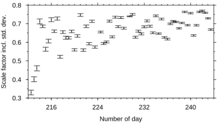
Fig. 1. The scale factors with standard deviation.

a first approximation it is acceptable to neglect this compo-nent of the non-conservative forces. This seems acceptable because the main part of the non-conservative forces is due to air drag which is measured by the along-track component of the acceleration. The air drag can be estimated

Fa= Z

|v|aydt (5)

|_{v| is the magnitude of the velocity vector and ay}the along-track acceleration. The error induced by this approximation is due to the fact that the velocity vector not necessarily is aligned in the flight direction at all times. However the devi-ation is very small and therefore insignificant.

The along-track acceleration has to be corrected for bias and scale factor errors. The bias is found not to vary over the period, so the bias given in the accelerometer files is used,

b = 0.3555 mGal. The scale factor may have variations

(Visser and van den IJssel, 2002) and a value is estimated for the given period. The scale factor is estimated by correlating the air drag with the difference between the calculated grav-itational potential and an a priori gravity model. EGM96 is used as a priori gravity field model. A scale factor is esti-mated for each half day, see Fig. 1. Most of the values are between 0.6 and 0.8. Why the first three half days have so small scale factors are not explained yet. We therefore dis-regard these three values when finding the mean scale factor which is to be used in the further data analysis. We find a scale factor of 0.68. The along-track acceleration is then cor-rected for the scale factor and the air drag is calculated.

During the data analysis it was found that there are errors in the published accelerometer file from 16 August 2001. We have chosen to include this day anyway since the largest error is in the cross-track acceleration. Using Fourier analysis we found a signal corresponding to twice per obital revolution. This may be due to velocity or orbit errors. We have chosen to disregard this until further investigations have been made. The gravitational potential in satellite altitude is now esti-mated using Eq. (1) and may be used for the determination of spherical harmonic coefficients.

10-2 10-1 10-1 100 101 102 103 mGal 2 0 10 20 30 40 50 60 70 80 90 Degree 10-4 10-3 10-3 10-2 10-1 100 101 mGal 2 0 10 20 30 40 50 60 70 80 90 Degree

Fig. 2. Error degree variances (above) and degree variances (below)

for UCPH2002 04 (solid), EGM96 (dashed) and EIGEN-2 (dotted).

3 Gravity field model UCPH2002 04

As a preparation for the use of least squares collocation EGM96 to degree and order 24 was subtracted. This makes the residual potential statistically more homogeneous. The residual potential values are then up-/downwards continued to a common height of 440 km above the ellipsoid. The up-/downwards continuation is performed using gravity distur-bances calculated using EGM96.

The values in a grid spanning the earth from 87◦S to 87◦N with 0.5◦ spacing was determined using collocation. From this grid we estimate the spherical harmonic coefficients and their associated errors. In the determination of the coeffi-cients Fast Spherical Collocation is used. After the estima-tion EGM96 to degree and order 24 is added to get a com-plete set of spherical harmonic coefficients.

3.1 Evaluation of the UCPH2002 04 model

Degree variances and error degree variances of our model are compared with EGM96 and EIGEN-2 (Reigber et al., 2002), see Fig. 2. It is seen by inspection of Fig. 2 that above de-gree 60 there is no or little information left in UCPH2002 04 and EIGEN-2. Furthermore it is seen that below degree 40 UCPH2002 04 is expected to improve EGM96.

90 60 30 0 30 60 90 -5 -4 -3 -2 -1 0 1 2 3 4 90 60 30 0 30 60 90 90 60 30 0 30 60 90 -180 -150 -120 -90 -60 -30 0 30 60 90 120 150 180 90 60 30 0 30 60 90 -180 -150 -120 -90 -60 -30 0 30 60 90 120 150 180

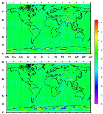
Fig. 3. Difference in geoid heights [m] between UCPH2002 04 and

EIGEN-2 (above) or EGM96 (below), respectively.

Using UCPH2002 04, EIGEN-2 and EGM96 to degree and order 60 we calculate geoid heights in a grid span-ning the earth from 87◦_{S to 87}◦_{N with 1.5}◦ _spacing.

Val-ues computed using EIGEN-2 and EGM96 are subtracted from the values computed with UCPH2002 04. These dif-ferences are shown in Fig. 3. The mean difdif-ferences between UCPH2002 04 and EGM96 is found to be −1.31 cm and be-tween UCPH2002 04 and EIGEN-2 −1.13 cm. The standard deviation of the differences is found to be 64.6 cm for both EGM96 and EIGEN-2.

The difference in Fig. 3 show a ribbon-like structure which we suspect is due to orbit errors in the RSO product. When inspecting the difference between UCPH2002 04 and EGM96 we find relativly large differences in Antarctica, the Himalayas and Baffin Bay as would be expected since only few oberservations were available in these areas when de-termining EGM96. When looking at the difference between UCPH2002 04 and EIGEN-2 there are some significant dif-ferences in Antarctica, Central and South-East Asia to be seen, but generaly UCPH2002 04 and EIGEN-2 agrees bet-ter than UCPH2002 04 and EGM96.

An earlier version of the model (UCPH2002 02) as well as other gravity field models has been compared with over 800000 terrestrial free-air gravity anomalies from Australia and New Zealand (Amos and Featherstone, 2003). These comparisons show that UCPH2002 02 and EIGEN-2 gives a better fit to the terrestrial data than other satellite-only gravity models. UCPH2002 02 is found to give a slightly better fit than EIGEN-2, but the difference is not statistically

signifi-4 E. Howe et al.: Analysis of one month of CHAMP state vector and accelerometer data cant. The UCPH2002 02 model uses a less accurate gridding

method than the current model.

4 Concluding remarks

We have determined a gravity field model from one month of CHAMP RSO and accelerometer data using energy conser-vation and collocation. The gravity field model is complete to degree and order 90. We find that our model is different from EGM96 in areas where it is known that for the determi-nation of EGM96 very little data were used. We find a good agreement between our model and EIGEN-2. UCPH2002 04 has new information compared to pre-CHAMP models and agrees with post-CHAMP models. It indicates that the en-ergy conservation method is feasible for gravity field recov-ery. However further investigations are still needed.

It is very important to reduce orbit and velocity error. This can be done with precise orbits. Some of the features in the polar regions may be caused by cross winds and the fact that the velocity vector deviates the most from the flight direction in these regions. This can be corrected by taking all three accelerations into account, since recently a correction for the erroneous radial component have become available.

The energy conservation method is a promising method for gravity field recovery which should be further investi-gated and developed for use on GRACE and GOCE data as well. When precise orbit data becomes available we intent to determine a new set of spherical harmonic coefficients con-tingently using a larger time period.

Acknowledgement. Thanks to the CHAMP data centre for

provid-ing the data. This paper is a contribution to the SAGRADA project sponsored by the Natural Science Council of Denmark.

References

Amos, M. and Featherstone, W.: Comparisons of recent global geopotential models with terrestrial gravity field observations over New Zealand and Australia, Geomatics Research Australa-sia, in print, 2003.

Bilitza, D.: MSIS-E-90 Atmosphere Model, http://nssdc.gsfc.nasa. gov/space/model/models/msis n.html, 2002.

F¨orste, C.: CHAMP accelerometer data preprocessing – level-2-data generation at GFZ Potsdam, Paper presented at the 1st CHAMP Science Meeting, 2002.

Gerlach, C., Sneeuw, N., Visser, P., and ˇSvehla, D.: CHAMP grav-ity field recovery with the energy balance approach: first re-sults, in First CHAMP Mission Results for Gravity, Magnetic and Atmospheric Studies, edited by C. Reigber, H. L¨uhr, and P. Schwintzer, pp. 134–139, 2003.

Han, S.-C., Jekeli, C., and Shum, C.: Efficient gravity field recov-ery using in situ disturbing potential observables from CHAMP, Geophysical Research Letters, 29, 2002.

Howe, E. and Tscherning, C.: Preliminary analysis of CHAMP state vector and accelerometer data for the recovery of the gravity po-tential, in First CHAMP Mission Results for Gravity, Magnetic and Atmospheric Studies, edited by C. Reigber, H. L¨uhr, and P. Schwintzer, pp. 140–145, 2003.

Jekeli, C.: The determination of gravitational potential differences from satellite-to-satellite tracking, Celestial Mechanics and Dy-namical Astronomy, 75, 85–101, 1999.

Lemoine, F., Kenyon, S., Factor, J., Trimmer, R., Pavlis, N., Chinn, D., Cox, C., Klosko, S., Luthcke, S., Torrence, M., Wang, Y., Williamson, R., Pavlis, E., Rapp, R., and Olson, T.: The development of the joint NASA GSFC and the na-tional imagery and mapping agency (NIMA) geopotential model EGM96, Tech. Rep. NASA/TP-1998-206861, NASA Goddard Space Flight Center, 1998.

Longman, I.: Formulas for computing the tidal accelerations due to the moon and the sun, Journal of Geophysical Research, 64, 2351–2355, 1959.

Michalak, G., Baustert, G., K¨onig, R., and Reigber, C.: CHAMP rapid science orbit determination - status and future prospects, in First CHAMP Mission Results for Gravity, Magnetic and Atmo-spheric Studies, edited by C. Reigber, H. L¨uhr, and P. Schwintzer, pp. 98–103, 2003.

Reigber, C., CHAMP newsletter, no. 4, http://op.gfz-potsdam.de/ champ/more/newsletter {CHAMP} {004}.html, 2001.

Reigber, C., Schwintzer, P., Neumayer, K.-H., Barthelmes, F., K¨onig, R., F¨orste, C., Balmino, G., Biancale, R., Lemoine, J.-M., Loyer, S., Bruinsma, S., Perosanz, F., and Fayard, T.: The CHAMP-only EIGEN-2 Earth Gravity Field Model, Submitted to Advances in Space Research, 2002.

Sans´o, F. and Tscherning, C.: Fast spherical collocation: A general implementation, IAG Symposia, 125, 131–137, 2002.

Visser, P. and van den IJssel, J.: Verification of CHAMP accelerom-eter observations, Submitted to Advances in Space Research, 2002.