Applying Bayesian estimates of individual transmission line outage rates

Applying Bayesian estimates of individual

transmission line outage rates

Kai Zhou

, James R. Cruise

, Chris J. Dent

, Ian Dobson

, Louis Wehenkel

, Zhaoyu Wang

, Amy L. Wilson

‡_{University of Edinburgh, Scotland} §_{University of Li`ege, Belgium}

Abstract—Despite the important role transmission line outages play in power system reliability analysis, it remains a challenge to estimate individual line outage rates accurately enough from limited data. Recent work using a Bayesian hierarchical model shows how to combine together line outage data by exploiting how the lines partially share some common features in order to obtain more accurate estimates of line outage rates. Lower variance estimates from fewer years of data can be obtained. In this paper, we explore what can be achieved with this new Bayesian hierarchical approach using real utility data. In particular, we assess the capability to detect increases in line outage rates over time, quantify the influence of bad weather on outage rates, and discuss the effect of outage rate uncertainty on a simple availability calculation.

I. INTRODUCTION

Transmission line outage rates are fundamental to electric power system reliability calculations. However, individual line outages are infrequent (roughly one per year), so that estimating the line outage rate in a straightforward way by dividing the number of outages by the time elapsed gives an annual outage rate estimate that is often too uncertain to be useful. Alternatively, a better estimate can be obtained by recording outages of an individual line over decades, but then the outage rate is averaged over such a long time that it is again not useful. This problem is commonly addressed by grouping or pooling together data for similar lines. This gives a much better estimate for an annual outage rate, but this outage rate is now averaged over that group of lines. For example, the annual outage rate for all lines of 230 kV in a region can be calculated, and this is useful for detecting reliability problems of that group of lines and for giving a typical value for those lines for reliability calculations. However, variations in individual line reliability within the group cannot be addressed.

It is intuitive that combining data for lines that are similar in some way should enable better estimates of individual line reliability. But the similarities are partial, and there are mul-tiple ways in which individual transmission lines are partially similar, including their length, rating, geographical location,

The authors gratefully thank the Isaac Newton Institute for Mathematical Sciences, Cambridge for support and hospitality during the programme Mathematics of Energy Systems where work on this paper was initiated. We gratefully thank Bonneville Power Administration for making publicly available the outage data that made this paper possible. The analysis and any conclusions are strictly those of the authors and not of BPA. This work was supported by EPSRC grant no EP/R014604/1.&#34. KZ, ID, ZW acknowledge support from USA NSF grants 1609080 and 1735354. LW acknowledges the support of F.R.S.-FNRS Belgium for his sabbatical year and from the Simons Foundation for his stay at the Isaac Newton Institute.

and proximity. Pooling does not work when there are multiple partial similarities. However, recent work [1] shows that the Bayesian hierarchical model can leverage multiple partial sim-ilarities to get better estimates of individual line outage rates from utility data. Typical results are that, for the lines with less frequent outages and using one year of data, the annual outage rate estimated with Bayesian methods has less than half the variance of the straightforward estimate. Another way to state this typical result is that the Bayesian hierarchical model for one year of data gives the same accuracy as the straightforward estimate for two years of data. Thus the Bayesian hierarchical model mitigates to some extent the problem of estimating individual line outage rates. This paper explores how much advantage can be gained from applying our method to give these improved line annual outage rates from utility data. In the following paper sections, we consider three problems:

1) Detecting lines with reduced reliability: We determine with statistical validity which lines have deteriorated reliability over time to better discriminate which lines should be consid-ered for further analysis and maintenance or upgrade.

2) Storm and no storm data: We often want to partition the data set to get more specific information, and we illustrate the capability of our proposed method in this regard by comparing line outage rates during storms with line outage rates when there is no storm.

3) Effects on reliability calculations: The Bayesian hierar-chical model not only gives better estimates of individual line outage rates but also gives the uncertainty of these estimates. We discuss a simple example of an availability calculation to illustrate the impact of these advantages on a system reliability calculation.

Bayesian methods use probability distributions to model uncertainty in parameters – for our application this means that rather than producing point estimates for the outage rate of each line, a probability distribution is estimated. These probability distributions incorporate knowledge of the outage rates and their uncertainty [2]. The mean of the probability distribution (the posterior mean) can be used as a point estimate of the outage rate. The probability distributions are estimated starting from a prior distribution (i.e., a distribution that incorporates any prior knowledge about the outage rates) and then updated to also incorporate the utility data by using Bayes’s rule. If there is a line with frequent outages producing a lot of outage data, then the calculated outage rate will be mostly determined by the outage data, and the effect of the

prior distribution will be small. If, more typically, the line has infrequent outages and the data is sparse, Bayesian methods can calculate a more accurate outage rate than non-Bayesian methods because any available prior information can be taken into account. The Bayesian method in [1] is a hierarchical model – data is shared across lines that have some partial sim-ilarity, such as similar location, proximity, rating, or length. As shown in [1], sharing data in this way can improve estimates of line outage rates. This is because the hierarchical model can learn from similar lines when estimating the outage rate for a line with little associated data. There is much more explanation of the Bayesian hierarchical model and the detailed results of applying it to estimate line outage rates in [1].

It is an advantage of Bayesian methods that they calculate probability distributions of line outage rates. The distribution of the line outage rate contains valuable information about the uncertainty of the point estimate, such as the standard deviation or credible interval of the estimate. This gives engineers insight into how much to trust the point estimates of line rates. Moreover, the distribution of the line outage rate can easily be sampled in Monte Carlo simulations of system reliability, ensuring that the uncertainty of the line rates is accounted for in the system reliability calculation.

There is previous research estimating outage rates using Bayesian methods. [3] and [4] use Bayesian methods to predict outage rates in a district given the system weather conditions. [5] presents a Poisson-gamma random field model to estimate outage rates of the 230 kV transmission lines within rectangu-lar subdivisions of the utility area. [6] proposes a hierarchical Bayesian Poisson regression to estimate individual failure rates of distribution lines, considering their dependence on age, tree density and loading. [7] gives interval estimates of outage rates of individual transmission lines given weather conditions using a credal network with imprecise priors, which is an extension of Bayesian networks. Other researchers estimate individual line outage rates based on analytical methods. [8] models the line outage rate based on physical outage mechanisms, and [9] uses an exponential function model for the failure rate considering the unexplained factors in the outage data.

Transmission line outage rates are correlated with each other in several ways. Lines in the power grid interconnect at substations, and some faults or substation arrangements may trip several lines at once. Multiple line outages can occur because of protection schemes. Moreover, lines in the same area experience similar weather conditions. There is some previous work on these correlations. Li [4] and Dokic [10] study pooled outage rates and model the dependence on the district. Ieˇsmantas [5] models geographical dependencies between the outage rates per kilometer of 230 kV lines in rectangular subdivisions of the area, and concludes that there is weak geographical correlation between these outage rates.

II. BAYESIAN HIERARCHICAL METHOD

This section summarizes from [1] the inputs and outputs of the Bayesian hierarchical method of estimating line outage

rates and some typical results. For reasons of space and com-plexity, all explanations and details of the Bayesian method itself are referred to [1].

A. Utility line outage data input to Bayesian model

This section outlines the utility line outage historical data and the line parameters and spatial dependencies that are input to the Bayesian hierarchical model. For more details, see [11]. Detailed outage data are routinely collected by utilities. For example, NERC’s Transmission Availability Data System (TADS) collects outage data from North American utilities. Here, we use some publicly available historical line outage data recorded by a North American utility [12] for 14 years since 1999. The data record forced and scheduled line outages, including names of outaged lines, outage start and end times and dates, names of the end buses of lines, line attributes such as length, voltage level, districts in which a line is, and outage cause codes. Some lines cross several districts. There are 549 lines outaging in the data with rated voltages of 69, 115, 230, 287, 345, and 500 kV.

We neglect the scheduled outages and momentary outages and only consider the forced non-momentary outages. If a line fails and recloses several times in one day, it only counts once. Table I shows an example of the outage data. Attributes for a line are voltage level, line length, and the utility district(s) in which the line is. We can also compute the network from the outage data [11] and calculate the distances along the network between any two lines. Two aspects of line proximity are modeled by matrices Σ1and Σ2. Σ1is based on the utility

dis-tricts. Lines in the same district are more likely to experience the same weather conditions. Σ2is based on network distance

between lines, which reflects both geographic proximity and the physical and engineering interactions in the network. B. Bayesian model outputs and sample results

The Bayesian model produces probability distributions for the outage rate of each transmission line. An example is shown in Figure 1. The mean outage rate of all lines is 0.60.

Figure 2 shows the 95% credible interval of annual outage rates λifor i = 1, 2, ..., 549. (As discussed in [13], the credible

interval is in multiplicative form; that is, the multiplicative factor φ is determined so that P [λi/φ ≤ ˆλi≤ λiφ] ≥ 95%.)

III. DETECTING OUTAGE RATE INCREASES

It is desirable to examine historical transmission line out-ages and judge whether the outage rate has increased and the reliability of the line has deteriorated. If there is a high chance that the outage rate has increased significantly, then the con-dition of this line should be evaluated and decisions about its maintenance, operational limits, or upgrade could be consid-ered1_{. This section applies Bayesian estimates to this problem.}

We divide the 14 years of utility data into the first 7 years and the last 7 years. Applying the Bayesian method for each line k, we obtain an outage rate probability distribution λ(1)_k 1_{Similarly, we note that detecting significantly decreased outage rates could}

TABLE I

SAMPLE OF THE OUTAGE DATA

Outage counts in different years

Line ID 1 2 3 4 5 6 7 8 9 10 11 12 13 14 Voltage(kV) Length(mile) District

1 0 2 0 0 1 0 0 1 1 4 2 0 1 0 500 38.43 WEN 2 1 2 0 0 0 0 0 0 0 0 0 0 0 0 230 7.62 COV . . . . . . . . . . . . . . . . . . . . . . . . . . . . . . . . . . . . . . . . . . . . . . . . . . . . . . 549 0 0 0 1 0 0 0 0 0 0 1 0 1 0 230 0.48 SAL 0.0 0.2 0.4 0.6 0.8 1.0 0.0 0.5 1.0 1.5 2.0 2.5

Annual outage rate

Probability

Fig. 1. Probability distribution of the outage rate for line number 12. The mean of the distribution is 0.42 per year and is used for a point estimate of the outage rate. The standard deviation is 0.15 and is used to quantify the uncertainty of the point estimate of outage rate.

0 100 200 300 400 500 0.001 0.010 0.100 1 10 Line Outage rates

Fig. 2. 95% credible intervals (blue bars) of outage rates and posterior means (black dots). Lines are ordered by the upper bounds of credible intervals.

for the first 7 years and an outage rate probability distribution λ(2)_k for the last 7 years. An example is shown in Figure 3.

1st 7 years 0.0 0.5 1.0 1.5 2.0 2.5 0.0 0.5 1.0 1.5 2.0

Annual outage rate

Probability

2nd 7 years

Fig. 3. The distribution of outage rates for one line in the first 7 years and in the second 7 years.

We are interested in the probability pk = P[λ

(2) k > κλ

(1)

k ] (1)

of the line k outage rate increasing by more than some factor κ. We will show results for κ = 1, κ = 1.5, and κ = 2. If λ(2)_k > κλ(1)_k , a larger value of κ indicates a more significant increase in the outage rate.

We evaluate the probability (1) empirically by sampling 10 000 times from the probability distributions λ(1)_k and λ(2)_k , which are assumed to be independent. That is,

pk ∼=

1

10 000[number of samples with λ

(2) k > κλ

(1) k ] (2)

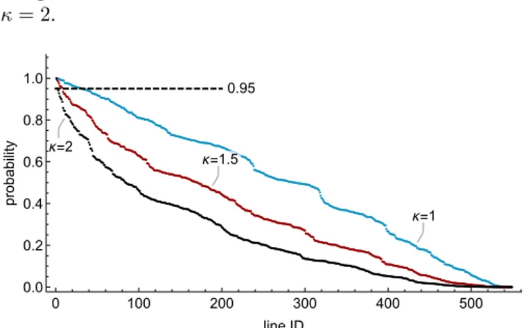
Figure 4 shows the probability pk for each line k. We

choose a significance level 0.05; that is, if pk > 0.95, λ (2) k

is significantly greater than κλ(1)_k , and we conclude that the outage rate for line k increases significantly in the last 7 years. According to this rule, we identify 31 lines with increased outage rates for κ = 1, 8 lines for κ = 1.5, and 1 line for κ = 2. κ=1 κ=1.5 κ=2 0 100 200 300 400 500 0.0 0.2 0.4 0.6 0.8 1.0 line ID probability 0.95

Fig. 4. The probability pkthat the outage rate increases by at least a factor

of κ in the second half time period from the first time period for each line k. Lines are ordered by the κ = 1 probabilities.

After identifying those lines with significant increases in outage rates, it is worthwhile checking the outage records to find out more about the possible specific causes of the increases, such as the cause codes for each outage. Utilities have much richer information about the outage and the grid conditions and can investigate much further. To illustrate this, we check the top three lines with the highest probability of outage rate increases. Table II shows the observed counts for these three lines, and there is an obvious increase in counts during the last 7 years. Outage causes for line 151 are mainly recorded as foreign utility and foreign trouble. Given the lack of outages in years 1 through 6, it should also be checked whether the line was newly installed in year 7. Line 138 has

various cause codes during the last 7 years, such as tree blown, line material failure, foreign trouble, and vegetable manage-ment. Line upgrade or tree-trimming may help lower the outage rate. Most of the causes for line 539 are wind related, so weather variations have a big influence on this line, and the line spacers, damping, and icing could also be reviewed.

TABLE II

OBSERVED OUTAGE COUNTS OF THE TOP THREE LINES WITH HIGHEST PROBABILITY OF INCREASES IN ANNUAL OUTAGE RATES

Line Outage counts in different years

ID 1 2 3 4 5 6 7 8 9 10 11 12 13 14

151 0 0 0 0 0 0 0 1 2 9 0 1 2 0

138 0 0 0 1 2 1 2 2 5 5 2 0 3 6

539 0 0 0 1 0 0 0 2 2 2 1 1 1 1

We compare the results with the conventional method, which estimates mean annual outage rates of individual lines by simply evaluating the average outage counts in a year. The standard deviation of the annual counts is also estimated. Then we fit a Gamma distribution for each line in each 7-year period using the method of moments. (Here we prefer the method of moments to maximum likelihood estimation because there are only 7 data points, and several of them are zeros; maximum likelihood estimation would exclude the zero observations, which reduces the information further and the optimization to find the maximum likelihood may fail.)

Note that the conventional method cannot deal with the lines with all zero counts in a 7-year period, while the Bayesian hierarchical model can solve this case. So we compare the two methods for lines with at least one nonzero count.

For each line in each 7-year period, we sample from the fitted Gamma distribution and use the same sampling method described at the beginning of this section to estimate the probability pk. We call this procedure the “basic method”

(the mean estimation is conventional, but we are not sure to what extent industry computes uncertainty of the conventional mean estimate). This basic method identifies 2 lines with increased outage rates for κ = 1, 1 lines for κ = 1.5, and no lines for κ = 2. Thus the increased uncertainty for the basic method detects significantly fewer lines with statistically verified increased outage rates.

The two lines identified by the basic method are line 539 and line 32. Line 539 is also identified in the above Bayesian method. The basic method does not identify line 151 because this line has no outage in the first 7 years. Line 138 is not identified by the basic method but is identified by the Bayesian method. The posterior distribution of the outage rate for line 138 has mean 0.81 and standard deviation 0.29 in the first 7 years, and mean 2.93 and standard deviation 0.62 in the second 7 years. Whereas in the basic method for line 138, the Gamma distribution has mean 0.86 and standard deviation 0.90 in the first 7 years, and mean 3.29 and standard deviation 2.14 in the second 7 years. The standard deviation of the posterior distribution is obviously lower than the standard deviation of the Gamma distribution. This low standard deviation makes the distributions in the two 7-year periods sufficiently different,

while the two Gamma distributions overlap due to their larger standard deviation.

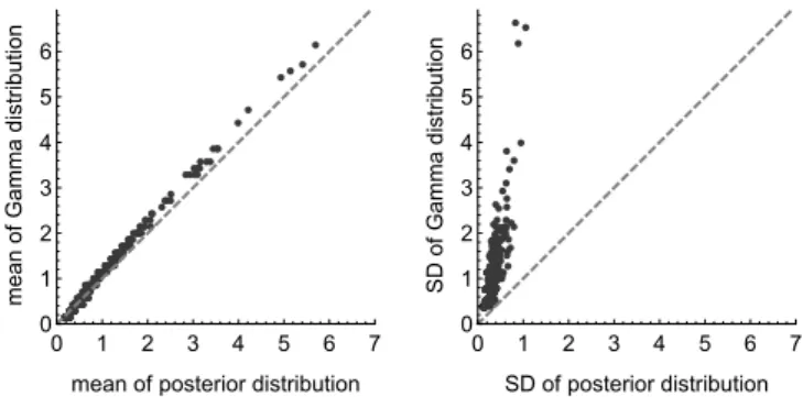
Figure 5 compares the means and standard deviations of the posterior distribution in the Bayesian method and the Gamma distribution in the basic method. Although the two methods have close means, the posterior distribution has a smaller standard deviation. This observation confirms the result in our journal paper [1] that hierarchical Bayesian estimates of outage rates have a lower standard deviation than the conventional estimates. The lower uncertainty of the Bayesian estimates explains why the Bayesian method more effectively detects lines with significant outage rate increases.

0 1 2 3 4 5 6 7 0 1 2 3 4 5 6

mean of posterior distribution

mean of Gamma distribution 0 1 2 3 4 5 6 7 0 1 2 3 4 5 6 SD of posterior distribution SD of Gamma distribution

Fig. 5. Comparing means (left panel) and standard deviations (right panel) of the posterior distribution and the Gamma distribution in two methods.

IV. EFFECT OF STORMS ON OUTAGE RATES

Since the proposed Bayesian hierarchical method mitigates the limited data problem in estimating individual outage rates, we can study further by investigating a subset of the outage data. For example, we can evaluate the effect of weather on outage rates.

We define a line outage as a storm outage if it occurs during a storm, otherwise it is called a non-storm outage. Then the annual storm outage rate is the number of storm outages divided by the total storm time in a year; similarly, the annual non-storm outage rate is the number of non-storm outages divided by the total non-storm time in a year. (Note that the Bayesian model does not directly produce the storm/non-storm outage rate. It outputs the average storm/non-storm outages over a year without considering the storm/non-storm time. So we need to divide the average storm/non-storm outages over a year by the storm/non-storm probability, which is the storm/non-storm time divided by the total time.)

The weather data is from the USA National Oceanic and Atmospheric Administration (NOAA) which includes storm events and other significant weather phenomena [14]. Using the method described in [15], we classify outages as storm outages and non-storm outages.

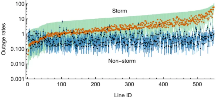
Figure 6 compares the storm and non-storm outage rates estimated using the Bayesian hierarchical model. 93% of lines have storm outage rates greater than non-storm outage rates (using the posterior mean as point estimation). The average storm outage rate is 4.5 per year which is nine times greater than the average non-storm outage rate 0.5 per year. This result

confirms the finding in [15] and provides more information due to the lower uncertainty of the Bayesian estimates.

Storm Non-storm 0 100 200 300 400 500 0.001 0.010 0.100 1 10 100 Line ID Outage rates

Fig. 6. 95% credible intervals of outage rates and posterior means (sorted according to the upper bound of storm outage rates). Orange crosses are storm outage rates, and black dots are non-storm outage rates.

The BPA data records the cause code reported for each outage. We now summarize how storms affect the cause codes. The proportion of cause codes “tree blown”, “wind”, “weather”, “ice”, “power system condition”, ”SCADA”, and “galloping conductors” for storm outages are at least one order of magnitude greater than that for non-storm outages; while the proportion of causes “equipment/miscellaneous”, “RAS initiated”, “human element”, “foreign utility”, “fire”, “smoke”, and “maintenance” for non-storm outages are at least one order of magnitude greater than that for storm outages. Fewer human errors are reported during storms, as “human element” is a cause for 0.08% of storm outages, compared to 1% for non-storm outages, and the proportions of “dispatcher” are about the same. Storms increase the outages caused by “SCADA” and “galloping conductors”, but do not increase other equipment causes such as “improper relaying”, “terminal equipment failure”, and “arc while switching”.

V. EFFECT OF OUTAGE RATE VARIATION ON A SIMPLE UNAVAILABILITY CALCULATION

This section shows how variation and uncertainty in outage rates affect an elementary transmission system reliability cal-culation. One of the simplest idealized availability calculations has 3 lines that minimally satisfy the N–1 criterion; that is, the system is available if all lines or 2 out of 3 lines are operating, and unavailable otherwise. The 3 lines are independent with exponential failure rates λ1, λ2, λ3and exponential repair rate

µ. State 1 is no lines out, states 2,3,4 are one line out, states 5,6,7 are two lines out, and state 8 is three lines out. The Markovian transition rate matrix Q is

            −λ1−λ2−λ3 λ1 λ2 λ3 0 0 0 0 µ −λ2−λ3−µ 0 0 λ2 0 λ3 0 µ 0 −λ1−λ3−µ 0 λ1 λ3 0 0 µ 0 0 −λ1−λ2−µ 0 λ2 λ1 0 0 µ µ 0 −λ3−2µ 0 0 λ3 0 0 µ µ 0 −λ1−2µ 0 λ1 0 µ 0 µ 0 0 −λ2−2µ λ2 0 0 0 0 µ µ µ −3µ            

The steady state probability distribution of states is given by the row vector π, where πQ = 0 and the entries of π add to one. The probability of unavailability is the sum of the last 4 entries of π. It is convenient to express the unavailability as the expected number of minutes of unavailability in a year by multiplying the probability of unavailability by 525 600, the number of minutes in a year.

In our raw line data, the mean outage rate is λ = 0.6 per year, and the standard deviation is 0.7. The mean restoration time is 907 minutes [16], which corresponds to the restoration rate of µ = 579 per year that we use throughout this section. We consider the effect of using an average outage rate for all three lines when their outage rates differ. A parameter α is used to control the variation of the line outage rates while keeping the mean outage rate constant. The outage rates in Table III satisfy λ2 = αλ1, λ3 = λ1/α, and

Mean{λ1, λ2, λ3} = 0.6 for several values of α. α = 5 gives a

plausible variation of outage rates (one standard deviation from the mean is 0.6±0.7) and approximately half the unavailability. That is, if the outage rates do vary according to α = 5, then using an average outage rate for all three lines approximately doubles the unavailability.

TABLE III

UNAVAILABILITY FOR SEVERAL ANNUAL OUTAGE RATES

α λ1 λ2 λ3 unavailability

1 0.6 0.6 0.6 1.7 min 2 0.51 1.03 0.26 1.4 min 5 0.29 1.45 0.06 0.8 min

We consider the effect of uncertainty in the estimated line outage rates on the unavailability. We model the uncertainty in estimates of λ1, λ2, λ3 by three independent Gamma

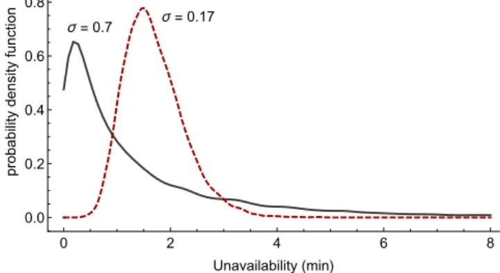
dis-tributions, each with mean 0.6 and standard deviation σ. The resulting probability distributions in the unavailability are shown in Figure 7 for σ = 0.7 and σ = 0.17. σ = 0.7 is the average of the standard deviations of individual transmission lines used in the basic estimation in section III. σ = 0.17 is the average of the standard deviations of individual transmission lines in the Bayesian estimation.

If we neglect the uncertainty in the estimated outage rates, the deterministic calculation with λ1 = λ2= λ3 = 0.6 gives

an unavailability of 1.69 minutes. If we use the average uncer-tainty σ = 0.17 that is typical of the Bayesian estimates, the 95% probability interval for the unavailability is {1.25, 3.01}. If we use the average uncertainty σ = 0.7 that is typical of that used in the basic method of section III, the 95% probability interval for the unavailability is {0.24, 8.63}. For this example, a typical uncertainty in the line outage rates appreciably affects the unavailability. The smaller uncertainty provided by the Bayesian estimates is clearly advantageous compared to the uncertainty provided by the basic method in section III.

We note that either the Bayesian or basic method considered above of estimating the standard deviation of individual line outage rates is better than conventionally estimating the outage rates of all the lines and computing the mean and standard

de-viation of this combined data. This procedure gives a standard deviation of 1.14, which is larger because it includes not only the uncertainty of individual line estimates but also the varia-tion in individual line outage rates from their combined mean. In the unavailability calculation, the larger standard deviation σ = 1.14 gives unacceptably large variation in the calculated unavailability, with a 95% probability interval {0.02, 14.27}.

σ = 0.7 σ = 0.17 0 2 4 6 8 0.0 0.2 0.4 0.6 0.8 Unavailability (min) probability density function

Fig. 7. Probability distributions of calculated unavailability for several values of standard deviation σ for the estimated line outage rate. The distribution of unavailability has standard deviation 2.6 for σ = 0.7 and standard deviation 0.56 for σ = 0.17. The mean unavailability is 1.69 minutes per year.

VI. CONCLUSIONS

The Bayesian hierarchical model can process standard trans-mission line outage data routinely collected by utilities to give improved estimates of individual line outage rates [1]. When the outage counts are low, the Bayesian hierarchical model estimates have lower variance than the conventional calculation of outage rate that simply divides counts of outages by the observation time elapsed. The Bayesian model does this by combining line data with data from other lines with partial similarities in rating, length, and proximity. This paper uses real utility data to explore several ways in which the improved performance of the Bayesian outage rates for individual lines can be exploited.

It is useful to be able to detect deterioration in line outage rates so that corrective action can be taken. We use the Bayesian outage rates to calculate the probability that an individual line outage rate has increased in a second 7-year period compared to a first 7-year period. Since the Bayesian outage rates have lower uncertainty, they can better detect significant outage rates increases in more lines than a basic conventional method. The significant increase in outage rate can be used to select lines that are likely to have deteriorated reliability in a principled way, so that these lines can be further investigated to inform upgrade, maintenance, modification, or derating decisions.

It is useful to split historical data sets for separate analyses to investigate the effect of factors such as storms. We illustrate the performance of the Bayesian method in distinguishing storm and no-storm outage rates. For our utility data, the average storm line outage rate is 4.5 per year, which is nine times the average non-storm line outage rate of 0.5 per year.

Bayesian methods calculate probability distributions of line outage rates, so that the mean gives a point estimate of the out-age rate and the standard deviation indicates the uncertainty of the point estimate. It is desirable to account for the uncertainty of outage line rate estimates in transmission system reliability calculations, and the Bayesian uncertainties are smaller than the conventional uncertainties. To start to discuss and quantify the effect of this on system reliability calculations, we contrast Bayesian hierarchical models and conventional methods for an elementary availability computation for a 3-line system. For this computation, using individual line outage rates as opposed to average outage rates for pooled data can halve the unavail-ability. Moreover, the reduced uncertainty of the Bayesian outage rates compared to conventional uncertainties gives significantly smaller probability intervals for the unavailability. Overall, our results indicate that the reduced uncertainty in individual line outage rates enabled by the Bayesian hier-archical model can be useful. We also expect that routinely quantifying the uncertainty in individual line outage rates will help to better justify decisions based on reliability calculations that depend on these outage rates.

REFERENCES

[1] K. Zhou, J. R. Cruise, C. J. Dent, I. Dobson, L. Wehenkel, Z. Wang, and A. L. Wilson, “Bayesian estimates of transmission line outage rates that consider line dependencies,” arXiv:2001.08681 [stat.AP], 2020. [2] A. Gelman et al., Bayesian data analysis. Chapman & Hall/CRC, 2013. [3] Y. Zhou, A. Pahwa, and S. Yang, “Modeling weather-related failures of overhead distribution lines,” IEEE Trans. Power Syst., vol. 21, no. 4, pp. 1683–1690, Nov. 2006.

[4] H. Li, L. A. Treinish, and J. R. M. Hosking, “A statistical model for risk management of electric outage forecasts,” IBM J. Res. Dev., vol. 54, no. 3, pp. 8:1–8:11, May 2010.

[5] T. Ieˇsmantas and R. Alzbutas, “Bayesian spatial reliability model for power transmission network lines,” Electr. Power Syst. Res., vol. 173, pp. 214–219, Aug. 2019.

[6] A. Moradkhani et al., “Failure rate estimation of overhead electric distribution lines considering data deficiency and population variability,” Int. Trans. Electr. Energ. Syst., vol. 25, no. 8, pp. 1452–1465, Apr. 2015. [7] M. Yang et al., “Interval estimation for conditional failure rates of transmission lines with limited samples,” IEEE Trans. Smart Grid, vol. 9, no. 4, pp. 2752–2763, Jul. 2018.

[8] R. Yao and K. Sun, “Toward simulation and risk assessment of weather-related outages,” IEEE Trans. Smart Grid, vol. 10, no. 4, pp. 4391–4400, Jul. 2019.

[9] Y. Wang et al., “Evaluating weather influences on transmission line failure rate based on scarce fault records via a bi-layer clustering technique,” IET Gen. Trans. Dist., vol. 13, no. 23, pp. 5305–5312, 2019. [10] T. Dokic et al., “Spatially aware ensemble-based learning to predict weather-related outages in transmission,” in Proc. 52th Hawaii Intl. Conf. System Science, Maui, HI, USA, Jan. 2019.

[11] I. Dobson et al., “Obtaining statistics of cascading line outages spreading in an electric transmission network from standard utility data,” IEEE Trans. Power Syst., vol. 31, no. 6, pp. 4831–4841, Nov. 2016. [12] “Bonneville Power Administration transmission services

operations & reliability website.” [Online]. Available: https://transmission.bpa.gov/Business/Operations/Outages

[13] I. Dobson, B. A. Carreras, and D. E. Newman, “How many occurrences of rare blackout events are needed to estimate event probability?” IEEE Trans. Power Syst., vol. 28, no. 3, pp. 3509–3510, Aug. 2013. [14] “NOAA national centers for environmental information storm events

database.” [Online]. Available: https://www.ncdc.noaa.gov/stormevents [15] I. Dobson et al., “Exploring cascading outages and weather via

process-ing historic data,” in 51st Hawaii Intl. Conf. Sys. Science, Jan. 2018. [16] S. Kancherla and I. Dobson, “Heavy-tailed transmission line restoration

times observed in utility data,” IEEE Trans. Power Syst., vol. 33, no. 1, pp. 1145–1147, Jan. 2018.