Gordon: CIRPÉE and Département d’économique, Université Laval, Québec, Canada G1K 7P4
Truchon: CIRPÉE and Département d’économique, Université Laval, Québec, Canada G1K 7P4
Cahier de recherche/Working Paper 06-24
Social Choice, Optimal Inference and Figure Skating
Stephen Gordon Michel Truchon
Février/February 2007
Abstract:
We approach the social choice problem as one of optimal statistical inference. If individual voters or judges observe the true order on a set of alternatives with error, then it is possible to use the set of individual rankings to make probability statements about the correct social order. Given the posterior distribution for orders and a suitably-chosen loss function, an optimal order is one that minimises expected posterior loss. The paper develops a statistical model describing the behaviour of judges, and discusses Markov chain Monte Carlo estimation. We also discuss criteria for choosing the appropriate loss functions. We apply our methods to a well-known problem : determining the correct ranking for figure skaters competing at the Olympic Games.
Keywords: vote aggregation, ranking rules, figure skating, Bayesian methods,
optimal inference, Markov Chain Monte Carlo
Contents
1 Introduction 1
2 The model 4
2.1 Vote aggregation . . . 4
2.2 Statistical models of voter choice . . . 6
2.3 The parameterised model of voter choice . . . 8
3 Loss functions 9 3.1 A generalised Kemeny loss function . . . 10
3.2 Discussion . . . 11
4 Posterior inference 13 5 An application to figure skating 14 5.1 National bias . . . 15
5.2 Parameter estimates . . . 16
5.3 Rankings estimates . . . 18
6 Conclusion 20 References 24 Appendix: Estimation algorithm 26
List of Tables
1 Loss function parameters and implications for costs of errors . . . 132 Parameter Estimates . . . 17
3 Optimal and ISU rankings: 1994 . . . 21
4 Optimal and ISU rankings: 2002 . . . 22
5 Costs of using a fixed rule: 1994 . . . 23
6 Costs of using a fixed rule: 2002 . . . 23
List of Figures
1 Losses associated with choices of η and θ . . . 121
Introduction
The question of how best to aggregate individual preferences is one of the oldest and best-known in the social sciences. This issue must be addressed in any setting in which decisions are to be made by social groupings: the election of political leaders and the allocation of communal resources are two of the best-known examples. The ranking of competitors in some judged sports, such as figure skating, presents the same methodological difficulty. It is well known, at least since Condorcet (1785), that it may be difficult to aggregate individual preferences into a coherent collective order, that is, to avoid cycles. Some two centuries later, Arrow (1963) crystallized this difficulty with his famous Impossibility Theorem, which demonstrates that there is no way of transforming individual preferences into a coherent social order, while respecting apparently innocuous prescriptions. This result does not imply that the social choice problem is any less relevant - as is testified by the abundant literature that his theorem has spurred.
If individual preferences are arbitrary, the Impossibility Theorem states that there is no way of resolving disagreements. But if we suppose that individuals observe a true social order with error, differences of opinion can be ascribed to random differences in perception. In this case, it should be possible to use individual voters’ reported rankings to infer the correct social order. That is, the social choice problem may be thought of as a statistical issue of optimal inference. This approach is as old as the social choice literature itself, and forms the basis for Condorcet’s justification of the majority principle. In this, he was certainly inspired by Rousseau (1913) in his Social Contract, for whom the opinion of the majority is legitimate because it expresses the “general will.”
When in the popular assembly a law is proposed, what the people is asked is not exactly whether it approves or rejects the proposal, but whether it is in conformity with the general will, which is their will. Each man, in giving his vote, states his opinion on that point; and the general will is found by counting votes. When therefore the opinion that is contrary to my own prevails, this proves neither more nor less that I was mistaken, and that what I thought to be the general will was not so. [Rousseau (1913), p. 93]
Condorcet’s rigorous formulation of this proposition is one of the earliest applications of the calculus of probability and of the maximum likelihood approach to inference. He assumed that every voter chooses the best of two alternatives with a probability larger than one half, and that this judgment is independent between pairs and voters. If the binary relation obtained by applying the simple majority rule to each pair of alternatives is an order, then it is the solution to the problem, that is, the most probable order.
Condorcet was perfectly aware that the binary relation resulting from his procedure may contain cycles, a phenomenon sometimes referred to as the Condorcet paradox. He proposed a method for breaking these cycles, but unfortunately this method gives consistent results only for the case of three alternatives. Young (1988) shows that a correct application of the maximum likelihood principle leads to the selection of rankings that have the minimal total number of disagreements with those of the voters. In other words, they minimise a “distance” proposed by Kemeny (1959) and for this reason, they are often called Kemeny orders. When it exists, that is, in the absence of cycles in the majority relation, the Condorcet ranking is the unique Kemeny ranking.
Drissi and Truchon (2004) relax the assumption that the probability of comparing cor-rectly two alternatives is the same for any pair of alternatives. They let the probability increase with the distance between two alternatives in the allegedly true ranking, thus al-lowing for the possibility that it may be more difficult to correctly rank two competitors who are ‘close’. They postulate a two-parameter probability function and they analyze the behaviour of the maximum likelihood rule as a function of these parameters.
We extend the standard Condorcet-Kemeny-Young approach in three ways:
• First, we add a third parameter to the probability function of Drissi and Truchon to take into account the possibility that judges may have a bias for alternatives with certain features, such as a shared nationality.
• Second, we use the reported votes to estimate the parameters of this probability func-tion.
• Third, we formalize and make explicit the optimal inference problem facing the decision-maker. Towards this end, we propose a family of two-parameter loss functions, and we discuss which parameter combinations might be most plausible in our application. Concerning the third point, the maximum likelihood principle yields an optimal order only for the special case in which the decision-maker’s loss function is degenerate, that is, uniform throughout the space of incorrect orders. If the true order on the set {a, b, c, d} is abcd, this loss function says that choosing dcba and abdc are equally costly. It is unlikely that a decision-maker would view reversing the last two candidates as being as serious an error as reversing the entire ranking.
Given the decision-theoretic nature of the problem addressed here, Bayesian methods provide a natural framework for our analysis. The decision-maker observes the ranking reported by voters or judges and computes the conditional distribution of the correct ranking conditional on this information. Given this distribution and a suitably-chosen loss function,
the optimal ranking is the order that minimises posterior expected loss.1
We apply our methods to a well-known - and occasionally notorious! - social choice problem: ranking competitors in figure skating competitions. Most spectators are aware that skaters are ranked from the scores that they receive from a panel of judges. However, fewer may realise that, prior to the 2006 Olympics, these scores served only to obtain a ranking for each judge, and that these rankings were then aggregated with one of two complex procedures devised by the International Skating Union (ISU), the decision-maker in this context. These two procedures are genuine social welfare functions in Arrow’s sense. One of them has been studied extensively by Bassett and Persky (1994) and the two by Truchon
1The formulation of a ranking problem as an optimal statistical decision problem is not completely new. Bühlmann and Huber (1963) formulate a ranking problem in a similar way, but they confine their analysis to the degenerate loss function. We are not aware of other contributions along these lines. It is the case that distances between rankings have been used to conceive ranking or aggregation rules: the Kemeny rule is one example. Meskanen and Nurmi (2006) show that several other well known rules may be defined in the same way, but with a different distance. Truchon (2005) offers a brief survey of ranking rules based on distances, some of which have been derived in a unique way from a set of axioms. These distances are mostly used to find a median or a mean ranking for the rankings making up a profile of preferences or votes.
(2004). We compare the optimal rankings that we obtain with those given by the two ISU rules, and with the Kemeny and the Borda rules.
The paper has six sections. Section 2 outlines the statistical model and describes how the figure skating problem fits into our framework. We discuss our proposed loss function in Section 3. Section 4 describes how the information contained in the rankings reported by the various judges can be used to obtain the optimal ranking. Section 5 applies these techniques to the Olympic figure skating example, and Section 6 concludes.
2
The model
2.1
Vote aggregation
Let A = {1, 2, . . . , m} be a set of alternatives or candidates to be ranked. We denote by B the
set of binary relations on A, by B∗the set of complete and asymmetric binary relations on A,
and by L the subset of (linear) orders (complete, transitive and asymmetric binary relations)
on A.2 An order on A can be represented by a vector r = (r
1, r2, r3, . . .)or x = (x1, x2, x3, . . .)
where r1 and x1 are the rank of alternative 1, r2 and x2 the rank of 2, and so on.3
Let J = {1, 2, . . . , n} be the set of voters or judges. For each judge j, we have an order4
xj
∈ L, also called a vote. Equivalently, a vote xj
can be represented by an (m × m) binary
matrix Xj =£xjst ¤ s,t∈A where: xjst = 1 if xj s < x j t 0 otherwise
2With m alternatives, the cardinality of B∗and L are 2m(m−1)2 and m! respectively. The difference between the two is the number of cyclic binary relations in B∗.
3Throughout, we shall use r to represent the true ranking on A and x to represent a vote on A.
4In figure skating, judges may give the same rank to two or more skaters but, for data reasons discussed in Section 5.2, we limit ourselves to the case where votes are drawn from the space of linear orders.
Conversely, given a binary representation Xj of an order, we get the representation xj by setting xj s= m− Pm t=1x j
st.5 We shall use the two representations interchangeably.
A profile of votes is an array X = (x1, . . . , xn)
∈ Ln. A profile may also be written in
the binary form X = (X1, . . . , Xn) . Once the voters or judges have cast their votes, the
problem is to aggregate these votes into a final order. We formalize this idea in the following
definition.6
Definition 1 An aggregation or ranking rule is a function Γ : Ln→ L that assigns to each
profile X, a final order Γ (X) of the alternatives. Γs(X)represents the rank of alternative s
in the final order Γ (X) .
In order to define the minimum expected loss aggregation rule that we shall use in this study, we need a few additional concepts. Given a true order r, suppose that profiles are generated by a known distribution function f ( · |r) and that the decision-maker’s prior beliefs about r can be described by a prior distribution function π ( · ) . The likelihood function L is given by L(r; X) ≡ f (X|r) , which is the distribution function re-interpreted as a function of r, given X.
If the profile X is observed, the decision-maker will revise the prior according to Bayes’ rule. The posterior distribution function π( · |X) on L is given by:
π (r|X) = Pf (X|r) π (r)
s∈Lf (X|s) π (s)
∝ L (r; X) π (r)
Definition 2 A loss function is a mapping d : L2
→ R+ such that d (r, ˆr) ≥ 0 ∀ˆr 6= r and
d (r, r) = 0∀r. The value d (r, ˆr) is the loss resulting from the selection of order ˆr when r is
the true order.
5There is an abuse of notation in using xsto represent elements of a vector and xstto represent elements of a matrix but, given the one-to-one correspondence between the xj and the Xj, this should entail no confusion. Naming both judges and alternatives as 1, 2, 3, . . . is also an abuse of notation but this allows for simpler notations.
Definition 3 Given a posterior distribution function π( · |X) on L and a loss function d, an
order r∗ that belongs to
arg min ˆ r X ˜ r∈L π(˜r|X)d(˜r, ˆr) (1)
is an optimal order with respect to π and d. The correspondence M EL ( · ; π, d) : Ln → R
that assigns to each profile X, the subset arg min ˆ r
P ˜
r∈Lπ(˜r|X)d(˜r, ˆr) is the minimum expected
loss rule.
Remark 1 An interesting special case is obtained by considering an “all-or-nothing” or
naive loss function of the form
dN(ˆr, r) = κ if ˆr6= r 0 if ˆr = r (2)
for some κ > 0. In this case, the minimum in (1) is obtained by setting r∗ equal to the mode
of the posterior distribution π ( · |X) ; see Poirier (1995, pp 302-304). If the prior distribution
π (· ) is uniform throughout L, then the posterior π ( · |X) is proportional to the likelihood
function L( · ; X). In this special case, the problem in (1) reduces to the maximisation of the likelihood function. Put differently, the M EL rule turns out to be the maximum likelihood rule.
2.2
Statistical models of voter choice
This study adopts the Condorcet approach to the social choice problem and its extension by Drissi and Truchon (2004) in supposing that the true social order exists, but that judges observe it with error. Formally, we assume that there exists a non-decreasing function
p : {1, . . . , m − 1} → ¡12, 1¢ such that if r ∈ L is the true social order on A, then the vote
of judge j on a pair of alternatives (s, t) is a random variable ˜xjst ∈ {0, 1} with marginal
distribution: Pr¡x˜jst = 1 | r ¢ = p (rt− rs) if rs < rt 1− p (rs− rt) if rs > rt (3) Pr¡x˜jst = 0 | r ¢ = 1− Pr¡x˜jst = 1| r ¢
Put simply, p (rt− rs) is the probability that a judge orders alternatives s before t when s
has a higher rank than t in the true order, that is, when rs < rt.
If the votes Xj
are taken from B∗, that is, if cycles are permitted but not ties, and if the
elements of the binary matrix Xj are independently distributed, then the distribution of the
whole matrix Xj is:
c Pr¡Xj | r, B∗¢= Y s,t∈A rs<rt Pr¡x˜jst= x j st| r ¢ (4)
If we denote by Pr(L|r) the probability of generating an order from (4), then:
Pr(L|r) = X
Xj∈L
c
Pr(Xj|r, B∗)
The probability of drawing an order from L is therefore:
Pr(Xj|r, L) = Pr(Xj |r, B∗) Pr(L|r) if X j ∈ L 0 if Xj ∈ B∗\L (5)
Restricting the sample space to L, that is, imposing transitivity, implies that the elements
of Xj are no longer independently distributed, even though the joint probabilities are still
based on the product of the individual marginal probabilities. Consider the case where m = 3 and where we know that a judge has ranked alternative s ahead of t and t ahead of u. Even
if the marginal probability of ranking u ahead of s is some 0 < ˆpsu < 1, transitivity implies
that the conditional probability that the judge will rank s in front of u is equal to one. A more satisfactory approach might have consisted in specifying a probabilistic model on L directly. Given the number of alternatives that we shall consider, this would have represented a daunting task. The binary approach, which is often used in the literature on social choice, together with the elimination of incoherent relations, is adopted for practical
reasons.7 As we shall see in subsection 2.3, this choice allows us to specify and estimate a
parsimonious parametric model.
Finally, we suppose that judges produce their orders independently according to (3-5 ), so that the probability of a given profile X is:
f (X|r) =
n Y j=1
Pr(Xj|r, L) (6)
2.3
The parameterised model of voter choice
We adopt the logistic probability function8 of Drissi and Truchon (2004) and Truchon and
Gordon (2006). That is, we let the term p (rt− rs) in (3), which is the probability that a
judge j ranks s before t when rs< rt, take the form
pαβst (r) =
exp(α + β(rt− rs− 1))
1 + exp(α + β(rt− rs− 1))
(7) with α > 0 and β ≥ 0. If β > 0, the probability increases with the distance between s
and t in the true order, measured by rt− rs.9 When β = 0, the probability is constant.10
Larger values of α are associated with higher probabilities of correctly ordering two adjacent alternatives.
We denote the parameterised version of the votes distribution (6) by
f (X|r, λ) (8)
where λ = (α, β) is the vector of parameters.
8This function is widely used in empirical studies of binary data.
9See Marcus (2001) for another approach that uses a similar distance measure in determining rankings. 10In Remark 1, we pointed out that, with a uniform prior and the naive loss function dN, the M EL rule simplifies to the maximum likelihood rule. If, in addition, we use the function defined by (7) with β = 0 to generate the distribution f ( · |r) on L, then the MEL rule turns out to be the Kemeny rule. As shown by Young (1988), in the constant probability case, this rule is the same as the maximum likelihood rule.
3
Loss functions
Before we can formulate a meaningful answer to the question of whether or not a given order is better than another, we must first establish criteria for evaluating orders. If all incorrect orders have the same consequences, then the optimal strategy is to select the most probable order. Although choosing the most likely order may seem a plausible strategy, a loss function of the form (2) may be difficult to justify. For example, (2) states that reversing the entire
order for 10 competitors has the same cost as reversing the ranks of the 9th- and 10th-place
competitors. It is difficult to imagine situations in which loss functions of the form (2) can be said to genuinely represent the costs of choosing an incorrect order. This is especially true in figure skating.
There is no loss function, and consequently no single aggregation rule, that will be ap-propriate for all problems. For example, if the object of the exercise is to select the best candidate among a set of alternatives, there may be no loss in reversing the order of the second-place and last-place alternatives, as long as the highest-ranked competitor is cor-rectly identified. On the other hand, there are many applications - such as research grant competitions - in which resources are allocated as a function of the final order. In this case, reversing the order of any two candidates would have real costs. In figure skating, an obvi-ous priority is to make sure that the gold, silver and bronze medals are given to those who deserve them. But the allocation of medals is not the only consideration; there are several reasons for concluding that the loss function should be concerned with the entire order:
• From the athlete’s point of view, there may be monetary losses associated with incorrect rankings. It is typically the case that the financial support that athletes receive and their participation in future competitions are contingent on success in international competitions; a low ranking may result in a reduction of funding.
• From the point of view of the various national figure skating agencies, the number of competitors that a country may send to international competitions, as well as the right to nominate judges, depends on the previous performance of their skaters; see Zitzewitz (2006). If a skater from a given country receives a low ranking, it may result in reduced participation in future international competitions.
3.1
A generalised Kemeny loss function
The Kemeny metric is a sensible place to start in specifying a loss function. Let γst:L2
→ R,
be a function defined for every couple of alternatives (s, t) and every pair of orders (r, ˆr) by:
γst(r, ˆr) = 1 if rs< rt and ˆrs > ˆrt 0 otherwise
Then the Kemeny metric on L is the function dK :
L2 → R defined by: dK(r, ˆr) =X s∈A X t∈A γst(r, ˆr) (9)
Since the Kemeny distance between r and ˆr increases with the number of inversions
between two orders, it certainly represents an improvement over the naive distance (2). But, going back to our ten competitors example, the Kemeny metric does not distinguish where in the order the inversions take place: reversing the first two candidates or the last two in the true order has the same effect on the Kemeny metric. In many situations, an error on a bottom ranked alternative in the true order would be of less consequence than the same error on a top ranked alternative.
A more plausible loss function would be decreasing with respect to rs itself, that is, the
rank of alternative s in the true order, for a fixed value of Pt∈Aγst(r, ˆr) .11 In addition to
being increasing with respect to Pt∈Aγst(r, ˆr) and decreasing with respect to rs, we may
wish that d be concave, that is, increase at a decreasing rate, with respect toPt∈Aγst(r, ˆr),
or alternatively be convex. We may have similar desiderata for the change with respect to rs.
We define a class of parametric functions that offer much latitude in this respect. The
members of this class are the functions dηθ defined as follows:
dηθ(r, ˆr) =X s∈A Ã X t∈A γst(r, ˆr) !η (m− rs+ 1)θ, η ≥ 0, θ ≥ 0 11If m = 4 and r = (1, 2, 3, 4) , thenP4
t=1γ2t(r, ˆr) = 2 with ˆr = (3, 4, 2, 1) as well as with ˆr = (4, 3, 2, 1) . Thus, the fact that alternatives 1 and 2 are correctly ranked in the first ˆr while their order is reversed in the second is not taken into account in this partial sum. However, it is accounted for in the complete sum.
With these more general loss functions12, the rate at which the loss increases with the
partial sum Pt∈Aγst(r, ˆr) is controlled with the parameter η. Moreover, this number is
weighted by the term (m − rs+ 1)θ. Note that d1,0 = dK and, with the convention 00 = 0,
d00 = dN, where dK and dN are defined by (9) and (2) respectively.
Remark 2 If r = (r1, . . . , rm) is the true order, the maximum distance under dηθ is always
attained for ˆr = (rm, . . . , r1) , whatever the values of the parameters. Indeed, each term
P
t∈Aγst(r, ˆr)reaches its maximal value for ˆr = (rm, . . . , r1) ,that is, by completely reversing
the true order. In particular, d1,0(r, ˆr) = dK(r, ˆr) = (m− 1)m
2 .
Remark 3 As is well known, Kemeny (1959) also defines a “distance” δK between an order
xand a profile X by: δK(r, X) =Pnj=1dK(r, xj) .The rule that he proposes and that bears
his name consists in minimizing Pnj=1dK(r, xj) . As recalled in footnote 10, Young (1988)
shows that, in the constant probability case, minimising this “distance” is equivalent to maximising the likelihood function.
3.2
Discussion
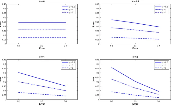
In order to get some intuition for plausible choices of η and θ, we consider the case where there are four alternatives. The errors associated with incorrectly reversing the first- and second-ranked, the second- and third-ranked and the third- and fourth-ranked alternatives are presented in Figure 1. In order to keep a common scale, the loss associated with reversing the true order (that is, getting each of the 6 possible pairwise orders wrong) is normalized to 1.
The parameter η determines the level of the curves drawn in Figure 1 while θ determines their slopes. For a given value of θ, an increase in η reduces the relative cost of making a particular inversion error. This is because increasing η increases the cost of completely reversing the true order proportionally more than is the case with any other error.
Figure 1: Losses associated with choices of η and θ 1-2 2-3 3-4 0 0.05 0.1 0.15 0.2 0.25 0.3 0.35 0.4 0.45 Error L o ss θ = 0 1-2 2-3 3-4 0 0.05 0.1 0.15 0.2 0.25 0.3 0.35 0.4 0.45 Error L o ss θ = 0.5 1-2 2-3 3-4 0 0.05 0.1 0.15 0.2 0.25 0.3 0.35 0.4 0.45 Error L o s s θ = 1 1-2 2-3 3-4 0 0.05 0.1 0.15 0.2 0.25 0.3 0.35 0.4 0.45 Error L o s s θ = 2 η = 0.5 η = 1 η = 2 η = 0.5 η = 1 η = 2 η = 0.5 η = 1 η = 2 η = 0.5 η = 1 η = 2
In our context, values of η greater than 2 are clearly implausible; we believe that the costs of making a mistake at the top end of the ranking are higher than what large values of
η would seem to imply. For the reasons described above, low values of θ are also probably
less plausible in our context.13
We believe that the (η, θ) combinations listed in Table 1 cover the plausible range, and these values will be used in the rounds of estimation below. Recall that (0, 1) corresponds to the Kemeny metric. Our preferred combination is (1, 1). However, we make no claims about the general applicability of our choice for other applications; other decision-makers facing
other problems would make other choices.14
13For more on the choice of the loss function, see Truchon (2005).
14In certain contexts, where we observe both the data and the analyst’s decisions, it may be possible to infer which combination of loss function parameter values are most consistent with the analyst’s behaviour. For example, Drissi (2002) includes an attempt to identify a loss function that would be consistent with the ISU-94 rule.
Table 1: Loss function parameters and implications for costs of errors
Parameters Ranking error
η θ 1st ↔ 2nd 2nd ↔ 3rd 3rd ↔ 4th 0.5 1.0 0.304 0.228 0.152 1.0 0.0 0.167 0.167 0.167 1.0 0.5 0.184 0.159 0.130 1.0 1.0 0.200 0.150 0.100 1.0 2.0 0.229 0.129 0.057
4
Posterior inference
The posterior distribution of interest for choosing the optimal order is π(r|X) - that is, the distribution of r conditional on the data, but unconditional on the parameters. If we apply Bayes’ rule to the data distribution in (8), we obtain the joint distribution:
π(r, λ|X) ∝ f(X|r, λ)π(r, λ) (10)
The distribution of interest is derived by integrating (10) with respect to the vector of fixed parameters λ = (α, β) . Since r takes on m! discrete values, calculating the posterior probabilities for each order would require m! rounds of numerical integration.
In the constant probability model (that is, with β = 0), this problem can be circumvented.
Indeed, if the priors are uniform, the Kemeny rule yields an order, say ˆrM L,that maximises
the posterior distribution (10) for all values of α > 0, that is, for all p > 0.5. It follows that ˆ
rM L is a most probable order a posteriori, so if the loss function has the “all-or-nothing” or
degenerate form (2), then ˆrM L is an optimal order.15
No similar results are available for variable probability models or for more general loss functions. The development of Bayesian Markov chain Monte Carlo (MCMC) techniques
provides a convenient method for estimating π(r|X) in the variable probability model.
Con-sider the sequence {rj, λj
}J
j=1 simulated according to:
rs ∼ π(rs|r−s, λ, X), s = 1, . . . , m
λ ∼ π(λ|r, X)
(11)
where r−s is the order obtained by excluding the component rs from r. Given certain
regu-larity conditions that are satisfied in our application16, it can be shown that the sequence
(rj, λj)
generated by (11) converges to the stationary distribution π(r, λ|X). A more detailed exposition is presented in the Appendix.
Let I[ˆr,r] denote the indicator function:
I[ˆr,r] = 1 if ˆr = r 0 if ˆr6= r Given J draws, r1, . . . rJ,
from the posterior distribution π(r|X), the estimator ˆ π(r = ˜r|X) = J−1 J X j=1 I[˜r,rj]
is a simulation-consistent estimator for π(r = ˜r|X). Thus, the estimate for the set17 of
optimal orders (1) takes the form: arg min ˆ r X ˜ r∈L d(˜r, ˆr)ˆπ(r = ˜r|X) (12)
5
An application to figure skating
The data used in this study come from the 1994 and 2002 Winter Olympic figure skating competitions. In these competitions, judges were asked to provide two sets of scores between 0 and 6 for each competitor, one for technical merit and the other for artistic presentation. These two scores were added and the sums sorted to produce the judge’s ranking of all the
16See Roberts and Smith (1994). The algorithm satisfies the sufficient condition that the conditional distributions in (11) have positive mass everywhere in the admissible region.
competitors. The final ranking was determined by the application of a rule set out by the International Skating Union (ISU). Two different sets of rules were used in 1994 and 2002.
We refer to the first as the ISU-1994 rule and to the second as ISU-98 rule18. These rules, as
well as the well-known Kemeny and the Borda rules, will be used as a basis for comparison with the M EL rule defined by (12).
An important feature of the ISU rules is that once a judge’s ranking has been determined, the actual scores are irrelevant in the determination of the final ranking. We assume that the judges are well aware of this fact and that data take the form of the rankings associated with each judge’s scores.
5.1
National bias
An additional factor that should be taken into account is the potential bias that judges may have in favour of competitors from their own home country. This sort of bias need not take the form of a conscious effort to manipulate the voting process; it may simply reflect variations in national styles. If a judge and a competitor have similar backgrounds, then it would be natural for the competitor to excel in aspects that were emphasised during his or
her training, and for the judge to reward it. This bias is denoted by Bi
st, where: Bsti =
1 if judge i and competitor s are from the same country and t is not
−1 if judge i and competitor t are from the same country and s is not
0 if neither s nor t are from the same country as judge i
0 if both s and t are from the same country as judge i
The possibility for national bias is incorporated into the model by modifying (7) according to
pλst(r) = exp(α + β(rt− rs− 1) + γBst)
1 + exp(α + β(rt− rs− 1) + γBst)
(13) where λ = (α, β, γ) is the new parameter vector.
5.2
Parameter estimates
We apply our model to 12 competitions: the short and long programs for the Men’s, Women’s and Pairs competitions at the 1994 and 2002 Olympics. We make use of priors that are uniform in both λ and r, and we assign zero prior probability to parameter combinations that violate the regularity conditions α > 0, β ≥ 0.
A feature of this data that has not yet been discussed are ties; we have assumed so far that judges are always able to clearly distinguish between two alternatives. But in our data set, judges do occasionally give identical scores to two competitors. The simplest way of dealing
with ties is to treat them as missing data.19 If voter i reports a tie between alternatives s
and t, we say that xist is a missing data point. These missing data points require only a
minor modification to the estimation algorithm (11); see the Appendix for further details. Our results are based on 6000 draws from the posterior (10) generated by (11); the first 1000
draws are discarded.20
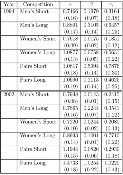
Table 2 lists estimates for the posterior means and standard deviations for the fixed parameters α, β and γ. Estimates for α range from 0.4479 to 1.1118. In the short programs, most estimates for β are quite small, suggesting that, when two competitors are far apart in the true order, it does not make it much easier for judges to correctly rank them. By comparison, in the long programs, the estimates for β are on average three times larger but by no means large. As for γ, those who are familiar with the controversies in figure skating judging will not be surprised to learn that this national bias parameter has a positive sign.
19Another way of incorporating ties would be to suppose that judges rank two candidates according to (3), that is without tie, with a certain probability ψ, and tie them with a probability of 1 − ψ. Although this completes the statistical model, it introduces an extra parameter ψ that is difficult to interpret: why would a voter report a tie? If ties are assigned to alternative pairs that are ‘too close to call’, then ψ would be an increasing function of d(s, t), thus requiring a further complication of the model. Preliminary attempts to model ties were abandoned when it became clear that there were too few ties to identify the parameters of the ties model with any degree of precision - indeed, some competitions had no ties at all.
20The numerical standard errors are about 1% of the estimates in Table 2; longer runs for selected com-petitions yielded virtually identical results.
Table 2: Parameter Estimates Year Competition α β γ 1994 Men’s Short 0.7466 0.1979 0.3164 (0.16) (0.07) (0.18) Men’s Long 0.8891 0.3105 0.6457 (0.17) (0.14) (0.25) Women’s Short 0.7618 0.0175 0.1851 (0.09) (0.02) (0.12) Women’s Long 1.0877 0.0758 0.5631 (0.13) (0.05) (0.22) Pairs Short 1.0817 0.5994 0.7876 (0.18) (0.14) (0.30) Pairs Long 1.0690 0.2113 0.4625 (0.19) (0.14) (0.25) 2002 Men’s Short 0.7938 0.0143 0.2415 (0.08) (0.01) (0.15) Men’s Long 0.7865 0.2244 0.3541 (0.16) (0.07) (0.22) Women’s Short 0.7220 0.0244 0.2080 (0.10) (0.02) (0.13) Women’s Long 0.8933 0.1001 0.7710 (0.14) (0.04) (0.22) Pairs Short 1.1944 0.0826 0.2930 (0.15) (0.06) (0.18) Pairs Long 1.4733 1.0254 1.0220 (0.18) (0.22) (0.43)
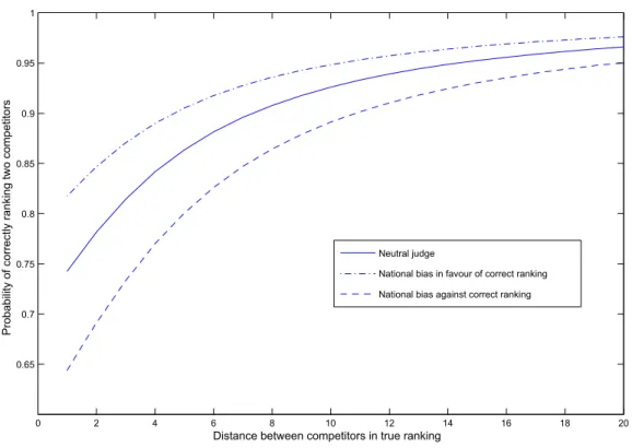
We now turn to the implications for these estimates on the choice probabilities. Figure 2 graphs the estimates from the 1994 long program for Pairs. These estimates are fairly representative of the range of variation in Table 2. Figure 2 suggests that the probability that an unbiased judge will properly rank two competitors who are adjacent in the true order is about 0.75, which appears plausible. This probability falls to 0.65 if he is biased against the higher-ranked skater, an effect that seems surprisingly small, although they are similar to what Campbell and Galbraith (1996) obtain.
Figure 2: Probability of reporting the correct binary relation 0 2 4 6 8 10 12 14 16 18 20 0.65 0.7 0.75 0.8 0.85 0.9 0.95 1
Distance between competitors in true ranking
P ro b ab ili ty o f co rr ec tly r an ki n g tw o co m p et ito rs Neutral judge
National bias in favour of correct ranking National bias against correct ranking
5.3
Rankings estimates
Theoretically, the solution to (12) requires searching across the m! possible values for r. In our data, m ranges from 17 to 28, so this would mean evaluating the expected loss of at
least 3.6 × 10¹⁴ possible orders - a daunting task. In order to simplify our analysis, we limit
attention to the set of orders that were visited by the MCMC algorithm.
As we noted earlier, the optimal order for a given problem will generally depend on the choice of the loss function. In the application at hand, the loss functions that we consider generally produce similar results. In what follows, we present results based on the combination (η, θ) = (1, 1).
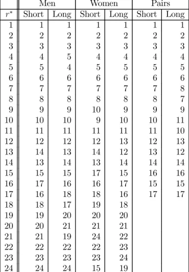
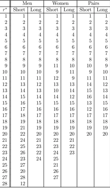
Table 3 compares the optimal order r∗ generated by (12) and those that were obtained
in the 1994 Olympics. In general, the two sets of rankings are quite similar: for example, they all yield identical rankings for the top three competitors. But there are a number of
inversions in the top ten. As noted in Section 3.1, these may have important consequences. Table 4 presents the same comparison for the 2002 Olympics.
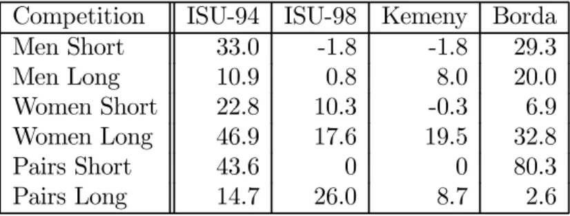
We next turn to the question of the possible ex post costs of committing to a fixed aggregation rule before the votes are observed. In principle, any fixed rule should fare worse - or at least, no better - than the solution to (12). But in practice, it is possible that our approach of limiting attention to the orders visited by the algorithm (11) may not yield a global optimum, for two reasons. Firstly, it may simply be that the MCMC algorithm did not run long enough to visit the global optimum; 5000 draws is a very small number compared
to the m! possible orders.21 Secondly, our statistical model excludes the possibility of ties,
and it could be that a ranking in which two or more candidates are ranked equally is in fact the solution to (12).
Tables 5 and 6 report the ex post expected losses associated with the ISU-94, ISU-98,
Kemeny and Borda rules22 for the two sets of competitions, expressed as a percent change
from the minimum in (12). Although there are several cases where using one of these benchmark rules provides slight gains, none of them consistently outperforms the minimum expected loss rule.
Nonetheless, it would appear that our strategy of limiting attention to the orders visited by our MCMC algorithm was perhaps too restrictive. Finding a way of extending the search in (12) to a larger - but still tractable - subset of L in order to increase the chances that (12) yields a global minimum would be a useful direction for future research.
21The computational burden of the MCMC algorithm being considerable, significantly longer runs are not feasible with the computing technology available to us.
22The first three rules can give multiple orders. When this happened, an order yielding the smallest expected loss was chosen. The Borda ranking is unique but can have ties. The ties were broken so as to
6
Conclusion
The main argument of this study is that in the Condorcet context -that is, where it is assumed that there is a true order that is observed with random error by voters - the social choice problem is one of optimal inference. Such a problem requires the specification of a well-defined statistical model, a loss function, and a method for identifying the order that minimises expected loss. The probability distribution used to evaluate this expectation will depend on the context. In this study, we focus on the posterior probability for the correct order, conditional on the observed votes.
Given the complex nature of the posterior in our application, we make use of standard Markov chain Monte Carlo techniques to simulate draws from the posterior distributions of interest, and these draws are used to calculate estimates for expected posterior loss. We find that this procedure produces plausible estimates for both the parameters of the probability distribution and the optimal order. Moreover, it is applicable to a broad class of vote distribution functions: it need not be supposed that the probability that a judge makes the correct pairwise ranking is constant in all contexts.
Our focus here is to illustrate some of the practical issues involved in an application of optimal inference methods to the social choice problem. The techniques developed here are fairly computationally-intensive, and ‘real-time’ results would only be available for low-dimension problems. Given the current state of computer technology and the number of competitors in a typical figure skating competition, the M EL estimator developed here is not yet a serious competitor for the other rules currently used.
Although the application in this paper is based on the ex post distribution p(r|X) — that is, after observing the data — our approach can also be extended to ex ante inference problems in which the decision-maker is interested in the behaviour of a given aggregation rule in repeated samples. This issue is taken up in Truchon and Gordon (2006).
Table 3: Optimal and ISU rankings: 1994
Men Women Pairs
r∗ Short Long Short Long Short Long
1 1 1 1 1 1 1 2 2 2 2 2 2 2 3 3 3 3 3 3 3 4 4 5 4 4 4 4 5 5 4 5 5 5 5 6 6 6 6 6 6 6 7 7 7 7 7 7 8 8 8 8 8 8 8 7 9 9 9 10 9 9 9 10 10 10 9 10 10 11 11 11 11 11 11 11 10 12 12 12 12 13 12 13 13 14 13 14 12 13 12 14 13 14 13 14 14 14 15 15 15 17 15 16 16 16 17 16 16 17 15 15 17 16 18 18 16 17 17 18 18 17 19 18 19 19 20 20 20 20 20 21 21 21 21 21 19 24 22 22 22 22 22 23 23 23 23 23 24 24 24 24 15 19
Note: In each competition, candidates are ordered according to the ranking generated by (12). The ISU ranking uses the ISU-94 rule, which was used in this competition.
Table 4: Optimal and ISU rankings: 2002
Men Women Pairs
r∗ Short Long Short Long Short Long
1 1 1 1 1 1 1 2 2 2 2 2 2 2 3 3 3 3 3 3 3 4 4 4 4 4 4 4 5 5 5 5 5 5 5 6 6 6 6 6 6 6 7 7 7 7 7 7 7 8 8 8 8 8 8 8 9 9 9 11 10 10 9 10 10 10 9 11 9 10 11 11 11 12 9 11 11 12 13 12 13 13 14 12 13 14 13 10 14 15 13 14 15 14 14 12 16 14 15 16 15 15 15 13 15 16 17 16 16 16 12 16 17 18 17 17 17 17 17 18 19 18 18 18 18 18 19 21 19 19 19 19 19 20 22 20 20 20 20 20 21 24 21 22 21 22 25 23 23 22 23 26 22 24 23 24 23 24 25 25 27 21 26 20 26 27 28 27 28 12
Note: In each competition, candidates are ordered according to the ranking generated by (12). The ISU ranking uses the ISU-98 rule, which was used in this competition.
Table 5: Costs of using a fixed rule: 1994
Competition ISU-94 ISU-98 Kemeny Borda
Men Short 33.0 -1.8 -1.8 29.3 Men Long 10.9 0.8 8.0 20.0 Women Short 22.8 10.3 -0.3 6.9 Women Long 46.9 17.6 19.5 32.8 Pairs Short 43.6 0 0 80.3 Pairs Long 14.7 26.0 8.7 2.6
Increase in expected posterior loss as a percentage of the loss associated with r∗.
Table 6: Costs of using a fixed rule: 2002
Competition ISU-94 ISU-98 Kemeny Borda
Men Short -7.9 -8.4 -8.4 -4.0 Men Long 17.1 -0.6 10.3 48.3 Women Short 17.8 -4.9 -6.7 5.5 Women Long 77.1 59.7 59.7 76.2 Pairs Short 88.0 88.0 111.8 94.3 Pairs Long -5.6 -5.6 -5.6 7.7
References
Arrow, K.J. (1963): Social Choice and Individual Values,” second edition, New York: Wiley. Bassett, W. and J. Persky (1994): “Rating Skating,” Journal of the American Statistical
Association, 89, 1075-1079.
Bühlmann, H. and P. Huber (1963): “Pairwise Comparison and Ranking in Tournaments,” Annals of Mathematical Statistics, 34, 501-510.
Campbell, B. and J.W. Galbraith (1996): “Nonparametric Tests of the Unbiasedness of Olympic Figure-Skating Judgments,” The Statistician, 45, 521-526.
Condorcet, Marquis de (1785): “Essai sur l’Application de l’Analyse à la Probabilité des Décisions Rendues à Probabilité des Voix,” Paris: De l’Imprimerie Royale.
Drissi-Bakhkhat, M. (2002), “A Statistical Approach to the Aggregation of Votes,” Ph D Thesis, Université Laval, Québec.
Drissi-Bakhkhat, M. and M. Truchon (2004), “Maximum Likelihood Approach to Vote Ag-gregation with Variable Probabilities,” Social Choice and Welfare, 23, 161-185.
Kemeny, J. (1959): “Mathematics without Numbers,” Daedalus, 88, 571-591.
Marcus, D.J. (2001): “New Table-Tennis Rating System,” The Statistician, 50, 191-208. Meskanen, T. and H. Nurmi (2006), “Distance from consensus: a theme and variations,”
http://www.congress.utu.fi/epcs2006/docs/A2_meskanen.pdf
Poirier, D.J. (1995): Intermediate Statistics and Econometrics: A Comparative Approach, Cambridge MA: MIT Press.
Roberts, G.O. and A.F.M. Smith (1994: “Simple conditions for the convergence of the Gibbs sampler and the Metropolis-Hastings algorithms,” Stochastic Processes and their Applications, 49, 207-216.
Rousseau, J.J. (1913): The Social Contract, London: J.M. Dent & Sons.
Truchon, M. (2004): “Aggregation of Rankings in Figure Skating,” Cahier de Recherche, 0402, Département d’Économique, Université Laval.
www.ecn.ulaval.ca/pages/Recherche/cahiers.html
Truchon, M. (2005): “Aggregation of rankings: A brief review of distance-based rules,” Cahier de Recherche 05-34, Centre interuniversitaire sur le risque, les politiques économiques et l’emploi (CIRPÉE).
Truchon, M. and S. Gordon (2006): “Statistical Comparison of Aggregation Rules for Votes,” Cahier de Recherche 06-25, Centre interuniversitaire sur le risque, les politiques économiques et l’emploi (CIRPÉE).
http://132.203.59.36/CIRPEE/cahierscirpee/2006/2006.htm
Young, H.P. (1988): “Condorcet’s Theory of Voting,” American Political Science Review,
82, 1231-1244.
Young, H.P. (1995): “Optimal Voting Rules,” Journal of Economic Perspectives, 9, 51-64. Zitzewitz, E. (2006): “Nationalism in Winter Sports Judging and Its Lessons for
Appendix: Estimation algorithm
The discussion in Section 4 assumed that all the reported binary relations in X are observed.
However, in our data set, we have several ties, which we treat as missing data. Let Xodenote
the profile of observed binary orders, and let Xu represent the unobserved data (that is, the
tie votes), so that X ≡ {Xo, Xu}. Since both Xu and λ are unobserved features of the
statistical model, we treat Xu as another variable to be estimated, requiring an extra step in
(11). The results in this study are based on the random sequence {rj, λj, Xuj}Jj=1 generated
by: rsj ∼ π(rs|r−sj−1, λj−1, Xuj−1, Xo), s = 1, . . . , m λj ∼ π(λ|rj, Xj−1 u , Xo) Xj u ∼ f(X|rj, λ j , Xo) (14)
We now turn to the question of how to simulate draws from the various distributions in (14)
As noted earlier, simulating draws directly from π(r|λ, Xu, Xo) would require evaluating 24!
probabilities; it is much faster to consider the orders on set of various alternatives in sequence.
If r−s is the vector of ranks of the m − 1 alternatives other than s, then the combination
{rs = i, r−s}, i = 1, . . . , m is an order for all m alternatives. Since we use uniform priors,
the individual order rs can be simulated from the discrete distribution defined by
Pr(rs= i|r−s, λ, Xu, Xo) =
f ({Xu, Xo}|λ, {rs = i, r−s})
Pm
i=1f ({Xu, Xo}|λ, {rs= i, r−s})
(15)
where f ({Xu, Xo}|λ, {rs = i, r−s}) is simply f(X|λ, r) defined by (6), where X = {Xu, Xo}
and r = {rs= i, r−s}. The entire order r is obtained by simulating draws from (15) for each
s = 1, . . . , m.Draws for the fixed parameters λ = (α, β, γ)0are generated by the random-walk
version of the Metropolis-Hastings algorithm. If αj−1 is generated by the previous iteration,
a candidate ˆαj is generated by a N (αj−1, σ2
α) proposing distribution. Define:
φα = min ½ f ({Xj−1 u , Xo}|ˆαj, βj−1, γj−1, rj) f ({Xuj−1, Xo}|αj−1, βj−1, γj−1, rj) , 1 ¾
The value for αj is determined by the rule:
αj =
( ˆ
αj with probability φα
αj−1 with probability 1− φα
Draws for β and γ are done sequentially, with acceptance probabilities φβ and φγ defined in
not satisfied, the acceptance probabilities for candidates violating these conditions is zero. After some preliminary calibrations, we found that setting the standard deviations of the
proposing distributions to σα = 0.15, σβ = 0.02, and σγ = 0.5 generated paths that mixed
well, and with acceptance rates between 0.4 and 0.5. Finally, given the order r and the