A Nonlinear Backstepping Controller of DC-DC Boost Converter for Maximizing Photovoltaic Power Extraction

(1)

ISMRE2018/XXXX-2018 ALGERIA

A Nonlinear Backstepping Controller of DC-DC

Boost Converter for Maximizing Photovoltaic

Power Extraction

Okba Boutebba

1

_{, Samia Semcheddine}

1

_{, Fateh Krim}

1

_{, Billel Talbi}

1

1_{Power Electronics and Industrial Control Laboratory (LEPCI), Electronics Dept., Setif-1 University, Sétif, Algeria,19000}

Corresponding Author: boutebbaokba@gmail.com

Abstract—The objective of this work is to integrate the backstepping control for tracking the maximum power point of a photovoltaic (PV) system. This control strategy is applied for a parallel DC-DC converter (type: boost) in order to regulate the output voltage of the PV generator, according to the reference voltage generated by the known Perturbation and Observation (P&O) MPPT (maximum power point tracking) algorithm. The nonlinear backstepping controller is based on Lyapunov function for ensuring the local stability of the system. The basic idea of the nonlinear backstepping controller is to synthesize a command law in a recursive way, that is to say step by step. This controller has a good transition response, a low tracking error, and a very fast response to the changes in solar irradiation and environmental temperature. To prove the effectiveness of the suggested control method, a comparative study through numerical simulations is presented with the classical PI (proportional-integral) controller.

Keywords— Boost converter, backstepping control, maximum power point tracking (MPPT), photovoltaic chain.

I. INTRODUCTION

In recent years, a very important development of renewable energies has occurred . With its inexhaustible potential and no negative impact on the environment [1], renewable energy is an appropriate and accessible technology for economic growth and sustainable development [2]. The study of the renewable energy conversion chain: primary energy extraction, electrical conversion, power generation, network transformation, and integration, is a basic element to improve the quality of production of "green" energy.

Given the current interest of the world in renewable energy in general and solar energy especially, PV panels are used today in plenty of applications. The PV array has a single operating point that can supply maximum power to the load. This point is named the maximum power point (MPP). The locus of this point has a nonlinear variation with temperature and solar radiation. Thus in order work array at the MPP, the PV system must include a maximum power point tracking (MPPT controller)

The boost type DC-DC converter is used generally in the PV system as adaptation stage [3-4]. The boost converter is connected to the output of the PV array and controlled by MPPT (Maximumm power point tracking) algorithm in order to achieve the optimum voltage for harnessing the maximum PV energy.

Numerous MPPT methods have been developed and proposed in the literature such as P&O algorithm [5], sliding

mode control (SMC) [6], fuzzy and artificial neural network methods [7-8] .

In this paper, a nonlinear backstepping controller, which modulates the duty cycle of a boost converter, is proposed. The output voltage of the solar array is the variable to be regulated; the output reference voltage of the PV is supplied by a P&O algorithm to obtain the MPP quickly, thus robustness is increased and Lyapunov's law ensures the global asymptotic stability and MPP is achieved even any

environmental conditions.

This paper is organized as follows: in the second section description of PV chain, PV panel and boost converter modeling are introduced, in section III, the backstepping control is detailed. Section IV is devoted to analysis of the simulation results and comparison with PI controller and finally the conclusion .

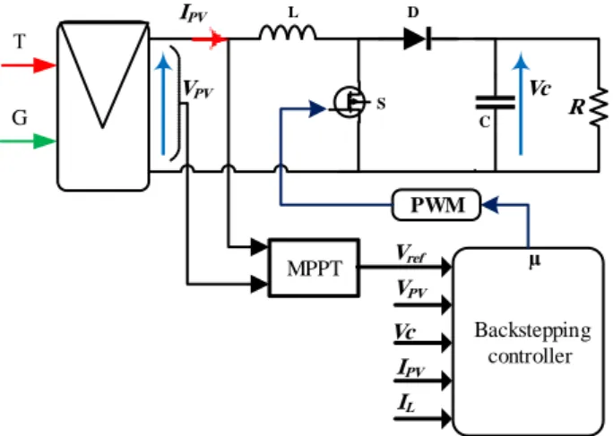
II. DESCRIPTION OF PHOTOVOLTAIC CHAIN The configuration of the PV chain under studied is given in Fig. 1. It represents a stand-alone structure composed of:

1. PV array which generates electric energy from solar energy.

2. DC-DC converter with resistive load controlled by backstepping controller to release the MPPT opera-tion. The backstepping controller block is the most important part of the system because it guarantees the necessary energy to the load.

MPPT G R Backstepping controller S D C L µ IPV VPV IPV IL Vref Vc VPV Vc PWM

(2)

A. PV Panel Modeling

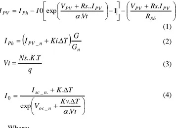
The PV panel used in this study is SIEMENS SM 110-24, which is simulated using the model proposed in [9]. This model includes a current generator in parallel with single diode, and series parallel resistance. The current generated by the PV panel can be expressed by the following equations:                         Sh PV PV PV PV Ph PV R I Rs V Vt I Rs V I I I 1 . . .. exp 0  (1)





n n PV Ph G G T Ki I I  _{_}  . (2)

q

T

K

Ns

Vt



..

.

(3)       _     Vt T Kv V T K I I n oc n sc . . exp . _ . _ 0  (4) Where: n T T T  

 (T and Tn are the actual and nominal

temperature respectively).

IPV_n, Gn, , Tn: are respectively the current generated by the

light, irradiation and temperature under nominal conditions.

VPV, IPV : are the PV output voltage and current respectively. Ki, Kv : are the current and voltage coefficients.

Voc_n, Isc_n : are respectively the open circuit voltage and

short-circuit current of the panel at nominal temperature.

I0 : dark saturation current.

Iph : photo-generated current.

Vt : thermal voltage.

Rs And Rsh : Series and Shunt resistance respectively. Ns: number of series cells in a PV panel.

α : diode quality factor.

q : electrical charge (q = 1,602. 10-19 Coulomb). K : Boltzmann’s constant (k = 1, 38. 10-23 J/K). T : Ambient temperature.

T : Effective cell temperature (Kelvin).

The PV array consists of several PV panels connected in series and parallel. Therefore, depending on PV panel model given by the equation (3), the PV array model can be represented as:                                                                   Npp Nss Rsh Npp Nss Ipv Rs Vpv Nss Nss Vt Npp Nss Ipv Rs Vpv Nss I N I N Ipv pp ph pp . . . 1 . . . . . exp 0 _  (5)

Where Nss, Npp are the number of PV panels connected in series and parallel respectively.

B. Modeling of boost DC-DC Converter

The boost converter is used to step-up a DC voltage [3]. In the proposed technique, a boost converter is used. This converter is used to shift the PV array output voltage (Vpv) to the desired Vmpp by changing the duty cycle with the help of the backstepping controller. The principal circuit diagram of the boost converter is shown in Fig. 2. It consists of the following main components:

1. Input voltage from PV (VPV).

2. Transistor switches (S). 3. Inductor (L). 4. Diodes (D1 & D2). 5. Capacitor (C1 & C2). 6. Load (R). L C1 Vpv S + -V0 D1 C2 D2 I0 I C 2 I C 1 IL IPV

Fig. 2. Boost converter

It is assumed that the converter is operating in continuous conduction mode (the current IL crossing the inductance

never get zero). There are two operating intervals of the converter i.e. interval 1, in which the switch is turned On, and interval 2, in which the switch is turned Off.

• interval 1, for the first period µTs: the IGBT switch (S) are ON, load is disconnected due to the closed path by switch (S). Inductor (L) is charged from PV through switch (S) in this mode.

Using kirchhoff’s voltage and current law, we can write

                 PV L L L PV PV V dt dI L V I dt dV C Ic I I dt dV C Ic 0 0 2 2 1 1 (6)

• Interval 2, for the second period (1-µ) Ts: the switch (S) are turned OFF and the load is connected to inductor (L) through diode (D2).

(3)

                  0 0 0 2 2 1 1 V V dt dI L V I I dt dV C Ic I I dt dV C Ic PV L L L L PV PV (7)

To find a dynamic representation valid for all the period

Ts, one generally uses the following averaging expression : Ts µ dt dx µTs dt dx Ts dt dx Ts µ µTs ) 1 ( ) 1 (     (8)

Applying the relation (8) to the systems of equations (6) and (7), we get the average model of the boost converter :

                 L V µ L V dt dI C I C I µ dt dV C I C I dt dV PV L L L PV PV 0 2 0 2 0 1 1 ) 1 ( ) 1 ( (9)            L V µ L x x C x C I x PV 0 1 2 1 2 1 1 ) 1 (       (10)

Where x = [x1 x2] T_{= [V}_{pv IL}_] T_{represents the state vector}

andµ [0,1] is the duty cycles of the signal control.

III. BACKSTEPPING CONTROL

In order to extract the maximum power from the PV module, a nonlinear backstepping controller is designed to track the PV array output voltage Vpv to Vmpp by controlling the duty cycle of the converter. For this purpose,

 Step 1

First of all, we define the error signal.

ref

PV V

V

e₁  (11)

Where Vref is the reference voltage generated by P&O algorithm. By converging the e1 to zero, we can get the

desired result.

Using the system (10), the tracking error derivative is written as follows: ref PV V x C C I e   ₂  1 1 1 1 (12)

The following lyapunov function is considered:

2 1 1 2 1 e V  (13)

In order to assure the asymptotic stability, the Lyapunov function must be positive definite and radially unbounded and its derivative with respect to time must be negative definite [10]. Taking the time derivative of equation (13), we get 1 1 1 ee V   (14)          PV _x _V_ref C C I e V ₂  1 1 1 1 1 (15)

From this equation for the derivative of Lyapunov function to be negative, it is necessary to

1 2 1 1 1 Ke V x C C I ref PV _ _  __ ₍₁₆₎ From where



K e Vref



IPV C x₂ ₁ ₁ ₁      (17)

Using the values of x2 from equation (17), equation (15)

becomes:









_           ref PV ref PV V I V e K C C C I e V 1 1 1   1 1 1 1 1 (18)            PV ref PV Vref C I V e K C I e V   1 1 1 1 1 1 (19) 2 1 1 1 Ke V  (20)

Since the derivative of V1 to be definitively negative, the

value of K1 must be defined positively, and equation (14)

must be satisfied.

β is the stabilization function, acts as a reference current for x2. then defined by:



K e Vref



IPV C     1 1 1



(21)

Hence the asymptotic stability of the system (10) in origin

 Step 2

The second error variable, which represents the difference between the state variable x2 and its desired value

β, is defined by:    ₂ 2 x e (22) Or    2 2 e x (23)

(4)





ref PV V e C C I e   ₂   1 1 1 1 (24) 2 1 1 1 1 1 1 e C V C C I e ref PV _ _ _     (25) 2 1 1 1 1 1 e C e K e   (26)

The derivative of e2 can define as follows



  ₂x₂  e (27) Therefore  2  1 (1 ) 0 1 1 V µ L x L e (28)





 ₂  1 x₁(1µ)V₀  L e (29)

To insure the asymptotic stability of the system and the convergence of the errors e1 and e2 to zero, a composite

Lyapunov function Vt is defined whose time derivative

should be negative definite for all value of x1 and x2.

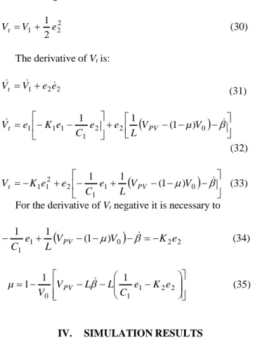
2 2 1 2 1 e V Vt   (30)

The derivative of Vt is:

2 2 1 e e V Vt     ₍₃₁₎





_   _ _ _             0 2 2 1 1 1 1 (1 ) 1 1 V µ V L e e C e K e V_t _PV (32)





                0 1 1 2 2 1 1 (1 ) 1 1 V V L e C e e K V_t _PV (33)

For the derivative of Vt negative it is necessary to



0



2 2 1 1 ) 1 ( 1 1 e K V V L e C  PV        ₍₃₄₎                    1 2 2 1 0 1 1 1 e K e C L L V V µ PV  (35)

IV. SIMULATIONRESULTS

In this section, numerical simulation of the PV chain shown in Fig. 1 is developed and implemented in MATLAB/ Simulink® enivrement. The PV array considered in this work consists of four identical PV modules shared into two parallel branches of two series connected modules. The

parameters for the PV module and the boost converter are indicated in Table 1. The backstepping controller parameters are shown in Table 2.

Table 1 . Pv module and the boost converter parameters.

Parameters Value

PV module

Maximum power (Pmpp)

Open circuit voltage (Voc)

Short circuit current (Isc)

Voltage at PMax (Vmpp)

Current at PMax (Impp)

Number of cells connected in series (Ns)

Number of cells connected in parallel (Np) 120 W 42.1 V 3.87 A 33.7 V 3.56 A 72 1 Boost converter Input capacitor C1 Output capacitor C2 Inductor L Load R 1100µF 1100µF 1mH 50Ω

Table 2. Backstepping controller parameters.

Parameters Value

K1 K2

3000 69980

A. Test under varying irradiance

Under this test, temperature is set constant at T= 25 °C and irradiance is changed abruptly after every 1.5 second. The varying levels of irradiance is shown in Fig. 3. Initial irradiance is G=1000 W/m², then it is decreased to G=400 W/m² at 1.5 second and finally it is increased to G=600 W/m² at 2.5 second and G=800 W/m² at 3.5 second.

It can be observed in Fig. 4, for each irradiance level, that the proposed controller tracks successfully the reference voltage. The performance of the proposed controller is then confirmed.

Fig. 5 illustrated the obtained result of PV array with

backstepping controller. It can be observed that the proposed controller has a very high performance at any level irradiation change , the controller performed well.

Fig. 6 shows the convergence of error signal e1 to zero under the abrupt variation of irradiance at 1 .5 second, 2.5 second and 3.5 second.

B. Test under varying tempurature

In this case, irradiance is set constant at G=1000 W/m2

while temperature is abruptly varied . Initial temperature is set at T= 5 °C, then it is stepped up to T=25 °C at 1.5 second and T=45 °C at 2.5 second and T=65 °C at 3.5 second.

Fig. 7 shows the varying levels of the temperature. From

PV array curves, the performance of the proposed controller (backstepping) is again confirmed, and good tracking to Vref shown in Fig. 8.

Fig. 10 shows the convergence of the error signal e to 1

zero under the variation of temperature at [1.5 ; 2.5 ; 3.5] second.

(5)

Fig. 3. Varying levels of irradiance.

Fig. 4. Tracking of VPV for different values of solar

irradiation.

Fig. 5. Power of PV array for different values of

solar irradiation.

Fig. 6. error signal e1 under varying irradiance.

Fig. 7. Varying levels of temperature.

Fig. 8. Tracking of VPV for different levels of

temperature.

Fig. 9. Power of PV array for different levels of

temperature.

(6)

V. COMPARISON WITH PI CONTROLLER

To show the performance of the backstepping controller, it is compared with (P&O/PI) controller. Both controllers are simulated and compared under varying temperature and irradiance levels.

A. Comparison under varying irradiance

In this comparison test, initially the irradiance is set at 1000 W/m² and is stepped down to 400 W/m² at 1.5 second , and set up to 600 W/m², 800 W/m² at 3 second.

Fig. 11 shows the Performance comparison of PI with the

backstepping controller. It can be seen that not only the proposed controller reaches the MPP more rapidly than the PI, but during the variation of irradiance at [1.5; 2.5; 3.5]second, the backstepping controller is rapidly with minimal oscillations. To see the comparative behavior after the variation of irradiance at all times, Fig. 11, Fig. 12 and

Fig. 13, Fig. 14 provides the zoomed view of PV power

,current Ipv and Vpv voltage and error signal e1 of the

both controllers. It can be seen that the robustness of backstepping controller is valid for all changes of the irradiation levels.

Fig 11. Backstepping vs PI power of PV array

under variation irradiance.

Fig 12. Backstepping vs PI tracking of IPV current.

Fig. 13. Backstepping vs PI tracking of VPV.

Fig. 14. Backstepping vs PI error signal e1 under

varying irradiance.

B. Comparison under varying temperature

In the second comparison test, both controllers are tested done under varying temperature levels. The irradiance is set constant at 1000 W/m² and temperature is stepped up from T= 5 °C to T = 25 °C at 1.5 seconds, and T=45 °C at 2.5 seconds to 65 °C at 3.5 seconds.

In Figs. 15 to 18, it can be seen that the proposed controller reaches our system in a minimal time with fewer oscillations as compared to PI controller.

On the same figures a zoomed view of the oscillations around the MPP of the two controllers.

Fig. 15. Backstepping vs PI power of PV array

(7)

Fig. 16. Backstepping vs PI tracking of VPV

Fig. 17. Backstepping vs PI error signal e1 under

varying irradiance

Fig. 18. Backstepping vs PI tracking of IPV current

VI. CONCLUSIONS

In this paper, robust and nonlinear backstepping based controller has been employed to track the MPP of a PV system. The PV array is linked to the load through a boost converter. To get maximum power from PV array, duty cycle of the boost converter is controlled through which the PV array output voltage is tracked to the voltage reference generated by the P&O method .

The asymptotic stability of the system is verified via Lyapunov stability analysis. The simulation results show that the controller performed well under the sudden variation of environmental conditions, which prove the good robustness of the proposed controller.

The comparison with the P&O/PI controller is made which shows that the proposed controller performed better during the variation in the climatic conditions (irradiance and temperature levels). As a future perspective, an implementation of the proposed controller using a dSPACE system be introduced.

Acknowledgement

This paper is a part of the project PRFU: A10N01UN190120180002.

REFERENCES

[1] A. Bahadori, C. Nwaoha, S. Zendehboudi, et G. Zahedi An overview of renewable energy potential and utilisation in Australia , Renew. Sustain. Energy Rev., vol. 21, p. 582‑589, mai 2013.

[2] P. A. Owusu et S. Asumadu-Sarkodie, A review of renewable energy sources, sustainability issues and climate change mitigation , Cogent Eng., vol. 3, no 1, p. 1167990, 2016.

[3] T.-F. Wu et Y.-K. Chen, Modeling PWM DC/DC converters out of basic converter units, IEEE Trans. Power Electron., vol. 13, no 5, p. 870–881, 1998.

[4] H. El Fadil et F. Giri, Backstepping based control of PWM DC-DC boost power converters , in Industrial Electronics, 2007. ISIE 2007. IEEE International Symposium on, 2007, p. 395–400.

[5] M. G. Villalva et E. Ruppert, Analysis and simulation of the P&O MPPT algorithm using a linearized PV array model , in Industrial Electronics, 2009. IECON’09. 35th Annual Conference of IEEE, 2009, p. 231–236.

[6] E. Bianconi et al., Perturb and observe MPPT algorithm with a current controller based on the sliding mode , Int. J. Electr. Power Energy Syst., vol. 44, no 1, p. 346–356, 2013.

[7] W. Dazhong et W. Xiaowei, A photovoltaic MPPT fuzzy controlling algorithm [J] , Acta Energiae Solaris Sin., vol. 6, p. 008, 2011. [8] A. B. G. Bahgat, N. H. Helwa, G. E. Ahmad, et E. T. El

Shenawy, Maximum power point traking controller for PV systems using neural networks , Renew. Energy, vol. 30, no 8, p. 1257–1268, 2005.

[9] S. Lalouni et D. Rekioua, Modeling and simulation of a photovoltaic system using fuzzy logic controller , in Developments in eSystems Engineering (DESE), 2009 Second International Conference on, 2009, p. 23–28.

[10] H. K. Khalil, Noninear systems , Prentice-Hall N. J., vol. 2, no 5,p. 5 –1, 1996.