HAL Id: inserm-01203004
https://www.hal.inserm.fr/inserm-01203004
Submitted on 22 Sep 2015HAL is a multi-disciplinary open access archive for the deposit and dissemination of sci-entific research documents, whether they are pub-lished or not. The documents may come from teaching and research institutions in France or abroad, or from public or private research centers.
L’archive ouverte pluridisciplinaire HAL, est destinée au dépôt et à la diffusion de documents scientifiques de niveau recherche, publiés ou non, émanant des établissements d’enseignement et de recherche français ou étrangers, des laboratoires publics ou privés.
SPEQTACLE: An automated generalized fuzzy C-means
algorithm for tumor delineation in PET
Jérôme Lapuyade-Lahorgue, Dimitris Visvikis, Olivier Pradier, Catherine
Cheze Le Rest, Mathieu Hatt
To cite this version:
Jérôme Lapuyade-Lahorgue, Dimitris Visvikis, Olivier Pradier, Catherine Cheze Le Rest, Mathieu Hatt. SPEQTACLE: An automated generalized fuzzy C-means algorithm for tumor delineation in PET. Journal of Medical Physics, Medknow Publications, 2015, 42 (10), �10.1118/1.4929561�. �inserm-01203004�
1
SPEQTACLE: an automated generalized fuzzy C-means
algorithm for tumor delineation in PET
Jérôme Lapuyade-Lahorgue1, Dimitris Visvikis1, Olivier Pradier1,2, Catherine Cheze Le Rest3, Mathieu Hatt1
1LaTIM, INSERM, UMR 1101, Brest, France
2 Radiotherapy department, CHRU Morvan, Brest, France
3DACTIM, Nuclear medicine department, CHU Milétrie, Poitiers, France
1
Corresponding author: M. Hatt 2
INSERM, UMR 1101,LaTIM 3
CHRU Morvan, 2 avenue Foch 4
29609 Cedex, Brest, France 5 Tel: +33(0)2.98.01.81.11 6 Fax: +33(0)2.98.01.81.24 7 E-mail: [email protected] 8 9
Wordcount: ~9400 (8900 for main body, 540 for appendix, 255 for abstract) 10
Disclosure of Conflicts of Interest: No potential conflicts of interest were disclosed. 11
Funding: No specific funding. 12
2 Abstract
13
Purpose: accurate tumordelineation in PET images is crucial in oncology. Although recent 14
methods achieved good results, there is still room for improvement regarding tumors with 15
complex shapes, low signal-to-noise ratio and high levels of uptake heterogeneity. 16
Methods: We developed and evaluated an original clustering-based method called 17
SPEQTACLE (Spatial Positron Emission Quantification of Tumor - AutomatiCLp-norm 18
Estimation), based onthe fuzzy C-means (FCM)algorithm with a generalization exploiting a 19
Hilbertian norm to more accurately account for the fuzzy and non-Gaussian distributions of 20
PET images.An automatic and reproducibleestimation scheme of the norm on an image-by-21
image basis wasdeveloped.Robustness was assessed by studying the consistency of results 22
obtained on multiple acquisitions of the NEMA phantom on three different scanners with 23
varying acquisitions parameters. Accuracy was evaluatedusing classification errors (CE) 24
onsimulated and clinical images. SPEQTACLE was compared to another FCM 25
implementation (FLICM)and FLAB. 26
Results: SPEQTACLE demonstrateda level of robustness similar to FLAB (variability of 27
14±9% vs. 14±7%, p=0.15) and higher than FLICM (45±18%, p<0.0001), and improved 28
accuracy with lower CE(14±11%) over bothFLICM (29±29%) and FLAB (22±20%) on 29
simulated images. Improvement was significant for the more challenging cases with CE of 30
17±11% for SPEQTACLEvs. 28±22% for FLAB (p=0.009) and 40±35% for FLICM 31
(p<0.0001). For the clinical cases, SPEQTACLE outperformed FLAB and FLICM (15±6% vs. 32
37±14% and 30±17%, p<0.004). 33
Conclusions: SPEQTACLE benefitted from the fully automatic estimation of the norm on a 34
case-by-case basis.This promising approach will be extended to multimodal imagesand 35
multi-class estimation in future developments. 36
Keywords: PET segmentation - clustering methods -Fuzzy C-means-Hilbertian norm. 37
3
Introduction
39
Positron Emission Tomography (PET) is established as a powerful tool in numerous 40
oncology applications1, including target definition in radiotherapy planning2, and therapy 41
monitoring3, 4, two applications for which tumor delineation is an important step, allowing for 42
instance further quantification of PET images such as the extraction of image based 43
biomarkers5–7. Within this context, automatic 3D functional volume delineation presents a 44
number of advantages relative to manual delineation which is tedious, time-consuming and 45
suffers from low reproducibility8.PET imaging is characterized by lower spatial resolution (~4-46
5mm 3D full width at half maximum (FWHM)) and signal-to-noise ratio (SNR) compared to 47
other medical imaging techniques such as Magnetic Resonance Imaging (MRI) or Computed 48
Tomography (CT). In addition, the existing large variability in scanner models and associated 49
reconstruction algorithms (and their parameterization) leads to PET images with varying 50
properties of textured noise, contrast, resolution and definition in clinical routine practice, 51
which becomes acritical issue in multi-centric clinical trials9. Thus, automatic, repeatable and 52
accurate, but also robustsegmentation of tumor volumes is still challenging.Many methods 53
based on various image segmentation paradigms, including but not limited to fixed and 54
adaptive thresholding, active contours and deformable models, region growing, statistical 55
and Markovian models, watershed transform and gradient, textural features classification, 56
and fuzzy clustering,have been already proposed10, 11. Despite the recent improvements and 57
the high level of accuracy and robustness achieved by some of these state-of-the art 58
methods, there is still room for improvement, especially regarding the delineation of tumors 59
with complex shapes, high level of uptake heterogeneity, and/or low imageSNR. 60
Methods including clustering and Bayesian estimation have demonstrated promising 61
performance in PET tumor volume segmentation. 62
On the one hand, in Bayesian segmentation methods, statistical distributions (also called 63
noise distributions)of the intensities are modeled by summarizing the histogram of the 64
4 images considering a reduced number of parameters to estimate. These methods provide 65
automatic algorithms allowing noise modeling and prior solution selection,which allows them 66
in turn to be less sensitive to noise than other segmentation approaches due to their 67
statistical modeling12.Bayesian segmentation methods can be viewed as regularized “blind” 68
statistical approachesin which the prior probability constraints the solution. This prior 69
distribution can be defined in different ways according to the targeted application, for 70
instance usinghidden Markov field or chain models where the prior distribution is a Markov 71
field distribution13. Relatively recent examples of such methods specifically developed for 72
PET include Fuzzy Hidden Markov Chains (FHMC) and the Fuzzy Locally Adaptive Bayesian 73
(FLAB) methods. In FHMC, the prior distribution was modeled using fuzzy hidden Markov 74
chains14, whereas in FLAB the 3D neighborhood of a given voxel was used to locally 75
estimate the fuzzy measurefor each voxel 15, 16, leading to a more accurate segmentation of 76
small structures. FLAB can be considered to be one of the state-of-the-art methods for PET, 77
according to its wide success due to its robustness, its repeatability and its overall accuracy 78
demonstrated on both simulated and various clinical datasets including radiotracers of 79
hypoxia and cellular proliferation 8, 16–23. 80
On the other hand, clustering methods aim at partitioning the images into clusters depending 81
on the statistical properties of the voxel intensities. The main interest of clustering methods 82
compared to Bayesian methods lies in their low computational cost, as well as easier 83
parameters estimation and overall implementation. The most known and used clustering 84
method is the K-means clustering which has been extended to Fuzzy C-means clustering 85
(FCM) by considering a fuzzy instead of a deterministic measure on the cluster’s 86
membership.The Fuzzy C-means (FCM) algorithm has several advantages including 87
flexibility and low computational cost. However, it fails to correctly address non-Gaussian 88
noise, geometrical differences between clusters, spatial dependency between voxels, as well 89
as the variability of fuzziness and noise properties or textures of the PET images that arise 90
5 from the large range of PET image reconstruction algorithms and post-reconstruction filtering 91
schemes currently used in clinical practice. 92
Regarding FCM more specifically, amongst the other different generalizations of FCM, some 93
incorporate a more accurate description of the clusters’ geometry in the data model, for 94
example by replacing the Euclidian norm by the Mahalanobis distance24. This method 95
requires estimating the covariance matrices of each cluster additionally to the centers of the 96
clusters and therefore takes into account that the clusters are not necessarily of identical 97
sizes. Another version uses the Lebesgue l1 andl norms instead of the Euclidian norm25. 98
Other authors have proposed to replace this Euclidian norm by a Hilbertiankernel26, which is 99
more reliable in cases where the data does not follow a Gaussian mixture model. Finally, 100
other authors have replaced the probability measure by evidential measure as in the 101
“possibilistic” FCM27. This last approach is interesting within the context of evidential theory, 102
however the way hard decision is carried out is heuristic and difficult to justify28. Amongst the 103
methods exploiting the spatial information, it was proposed to generalize FCM by introducing 104
spatial constraints to regularize it29. Other methods, such as the Fuzzy Local Information C-105
Means (FLICM)algorithm, incorporate in the minimization criteria the distance between 106
voxels30. 107
The goal of this work was to focus on FCM and to propose a novel generalization in order to 108
improve on the accuracy without sacrificing on robustness of PET tumor segmentation 109
results compared to current state-of-the-art techniques, for challenging heterogeneous 110
tumours.We have chosen to generalize FCM using a Hilbertian kernel,with the norm 111
parameter not set empirically or a prioribut rather estimated on an image-by-image basis, 112
using a fully automatic scheme based on a likelihood maximization algorithm. The new 113
algorithm was compared to FLICM and FLAB in terms of robustness and accuracy on real 114
and simulated PET image datasets. 115
6
Materials and methods
116
A. FCM algorithm and its extensions 117
Classical FCM algorithm
118
The FCM algorithm consists in finding for each classi
1 , ,C
, where C is the number of 119classes, and for each voxel
u
V
of the finite set of voxelsV 3, the centers
i
and 120the degrees of belief
p
u,i
[
0
,
1
]
minimizing the criterion: 121
V u C i i u m i uy
p
1 2 ,
(1) 122under the constraint:
1
1 ,
C i m i up
, 123where
y
u is the observed intensity for the voxel u and the parameterm
1
controls the 124fuzzy behavior and is usually chosen as
m
2
. 125Thedetails regarding this minimization are provided in appendix A. 126
Regarding the segmentation, for each voxel
u
V
, the class i
1 , ,C
maximizing the 127probability
p
u,i is chosen. This decision step is the same for the generalized FCM (GFCM). 128FCM as a Bayesian inference method
129
The traditional “hard” K-means clustering is equivalent to a Bayesian method where the 130
observations are modeled as a Gaussian mixture. FCM clustering can also be rewritten in 131
order to highlight a prior distribution regarding the parameters
p
u,iand
i, and a likelihood132
associating observations with the parameters. This idea has already been exploited by 133
choosing prior distributions to optimize the estimation31. The minimization of eq. (1) is 134
equivalent to the maximization of: 135
7
V u C i i u m i uy
p
f
P
1 2,
, where f is a positive function such thatP
is a probability 136density according to the observed variables
(
y
u)
uV called “likelihood”. From statistics, the 137maximization of
P
is equivalent to a likelihood maximization and is exhaustive (i.e. uses the 138entire information of the sample) if the density of
(
y
u)
uV maximizes the Shannon entropy. 139Moreover, one can show that a distribution whose form is given by 140
V u C i i u m i uy
p
f
P
1 2,
is an elliptical distribution (i.e.isodensities are ellipsoid) with 141 center
C i m i u C i i m i up
p
1 , 1 ,
and dispersion given by
C i m i u p 1 , 1. An elliptical distribution is entirely 142
determined by its functional parameter f , its center and its dispersion. Amongst the elliptical 143
distributions with the same center and dispersion, one can show that the maximum entropy is 144
reached if f is an exponential function. 145
Consequently, in this case, the minimization of eq. (1) is equivalent to the maximization of: 146
V u C i i u m i u V u C i i u m i uy
p
y
p
P
1 2 , 1 2 ,2
1
exp
2
1
exp
(2) 147 Also: 148
C i m i u C i i m i u C i m i u C i u i m i u u C i m i u C i i u m i u p p p y p y p y p 1 , 1 2 , 1 , 1 , 2 1 , 1 2 , 2
. 1498 Consequently, conditionally to the parameters, the observations
y
u are independent and 150Gaussian distributed as: 151
C i m i u C i m i u C i i m i u C i i u C i i up
p
p
N
p
y
p
1 , 1 , 1 , 1 , 11
,
:
)
)
(
,
)
(
(
(3) 152Whereas the prior distribution for parameters is given by: 153
C i C i m i u C i i m i u i m i u V u C i m i u V u C i i u C i i p p p p p p 1 1 , 2 1 , 2 , 1 , , 1 , 1 2 1 exp 1 ) ) ( , ) ((
154Drawbacks of the classical FCM
155
The previous theory results in two major drawbacks: 156
(a). FCM clustering is equivalent to a maximum posterior estimation when the 157
observations follow a Gaussian distribution conditionally to the parameters. 158
Consequently, FCM leads to inaccurate estimation when the data are not Gaussian. 159
(b). Similarly, FCM clustering assumes that the observations are independent 160
conditionally to the parameters, leading to inaccurate segmentation in the presence of 161
spatial dependencies. 162
B. SPEQTACLE algorithm: an automatic Generalized FCM algorithm (GFCM) 163
In this work we investigated the advantage of generalizing FCM by considering the Hilbertian 164
p
l -norm instead of the Euclidian norm and providing an associated scheme that enables a 165
fully automated estimation of the norm parameter for optimal delineation on a case-by-case 166
basis, in order to reduce user interaction and avoid empirical optimization. Indeed, a user-167
9 defined choice of the norm parameter based on visual analysis seems challenging because 168
of its non-intuitive nature, and would suffer from low reproducibility. An alternative would be 169
to optimize empirically the norm value on a training dataset, although it is unlikely that a 170
single norm value would be appropriate for all cases. We have consequently developed an 171
approach to automatically estimate the norm value for each image. 172
The proposed algorithm is called Spatial Positron Emission Quantification of Tumor 173
volume:AutomatiCLp-norm Estimation (SPEQTACLE). 174
Principle of GFCM algorithm
175
In the GFCM algorithm, the minimization criterion becomes: 176
V u C i i u m i uy
p
1 ,
(4) 177where, the norm parameter
1
and with no solution for
1
. Moreover, the cluster centers 178i
cannot be estimated explicitly when
2
, whereas
2
corresponds to the standard 179FCM. When
2
and
2
, the centers are computed using the Newton-Raphson 180algorithm and gradient descent respectively (for details we refer the reader to Appendix B. 181
and C.). 182
Generalized Gaussian distribution
183
We assume that conditionally on the parameters
(
i)
1iC and(
p
u,i)
1iC the observation is 184approximately distributed as a generalized Gaussian distribution whose density is 185
10
y
y
exp
1
2
parameterized by a center =
C i m i u C i i m i up
p
1 , 1 ,
, a dispersion = 186 1 1 , 1
C i m i u p and a shape . 187Estimation of the norm
188
The estimation technique presented in the next section is based on the above generalized 189
Gaussian distribution. Contrary to the Gaussian case, it is only an approximation; indeed the 190
expression (4) can be expressed as a product of
C i m i u
p
1, and a term of form
u y only in 191
the Gaussian case, which corresponds to
2
. However, it becomes a generalized 192Gaussian distribution if
p
u,i
1
holds for only one class. This approximation is valid as long 193as the probabilities
(
p
u,i)
are not too far from the configurationp
u,i
1
. Consequently, the 194norm parameter has to be estimated from an area for which one can consider that
p
u,i
1
195holds. In practice, this area was automatically selected using a background subtraction 196
method in order to provide a first guess of the tumor region, as recently proposed32. In order 197
to simplify the estimation task, we have chosen to estimate the norm for this background-198
subtracted region, which is likely to correspond to a first estimation of the tumor region, and 199
set a single norm parameter value for all classes. 200
The next step involves the estimation of the different parameters using likelihood 201 maximization. 202 Let us denote
C i m i u C i i m i up
p
1 , 1 ,
and
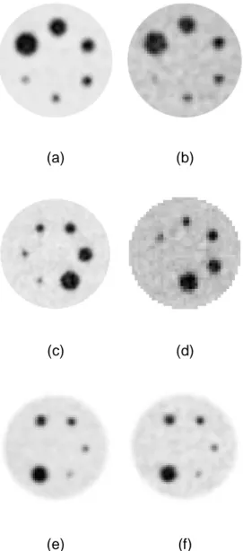
1 1 , 1
C i m i u p . 20311 First, one can assume that these values do not depend on u and secondly, that the 204
distribution of the observations
y
u in the selected area is approximately the generalized205
Gaussian distribution. Let
(
y
u)
uWbe the sample from the selected areaW
, the maximum 206likelihood estimators of, and, denotedˆML, ˆMLand ˆMLare solutions of the system: 207 a.
W u ML u ML u MLy
y
ˆ
)
ˆ
0
sgn(
ˆ 1 ; 208 b.
W u ML u ML ML ML MLy
W
ˆ ˆˆ
1
ˆ
ˆ
; 209 c.
W u ML ML u ML ML u ML ML ML ML MLy
y
W
ˆ ˆ 2ˆ
ˆ
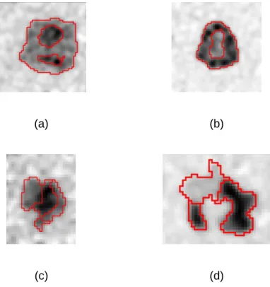
ˆ
ˆ
log
1
ˆ
ˆ
1
ˆ
, 210where,
W
is the cardinality ofW
and is the log-derivative of the Eulerian function (see 211AppendixD). 212
These equations are not linear and cannot be solved independently. Consequently, the 213
solution is estimated by using a combination of a variational method and the Newton-214
Raphson algorithm as outlined below: 215
1. Let
(0),
(0)and
(0)be the initial values ; 2162. From
( p), compute
(p1) by solving
W u p u p u p y y ) 0 sgn( ) ( ) 1 ( ) 1 (
using the 217 Newton-Raphson algorithm; 2183. From
( p)and
(p1), compute
W u p u p p py
W
) ( ) 1 ( ) ( ) 1 (
1
; 21912 4. From
(p1) and
(p1), compute
(p1)by solving 220
W u p p u p p u p p p p py
y
W
( 1) ) 1 ()
(
log
1
1
) 1 ( ) 1 ( ) 1 ( ) 1 ( ) 1 ( ) 1 ( ) 1 (
2215. Repeat steps 2, 3 and 4 until convergence. 222
Although such generalized Gaussian distributions have properties that allow for convergence 223
of the maximum likelihood estimation, the stopping criteria has to be defined. One could 224
assume that the estimation can be stopped when the successive values of
( p) (resp.
( p) 225and
( p)) are sufficiently close to each other, using the absolute distances as stopping 226criteria. However, the values of the parameters can be close, whereas the distance between 227
the resulting distributions may be large. Indeed, the smaller is, the more sensitive to the 228
value of
is the resulting density. To overcome this drawback, we used a more appropriate 229distance; namely the distance between distributions rather than the distance between 230
parameters’ values. This distance is defined from the Fisher information matrix(Appendix E). 231
It has been previously shown that the set of given parameterized distributions is a 232
Riemannian manifold whose metric tensor is given by the Fisher information matrix33. More 233
precisely, let
y
p
( y
)
:
be a smooth manifold of statistical distributions 234parameterized by an open setk, the distance between “close” distributions 235
)
(
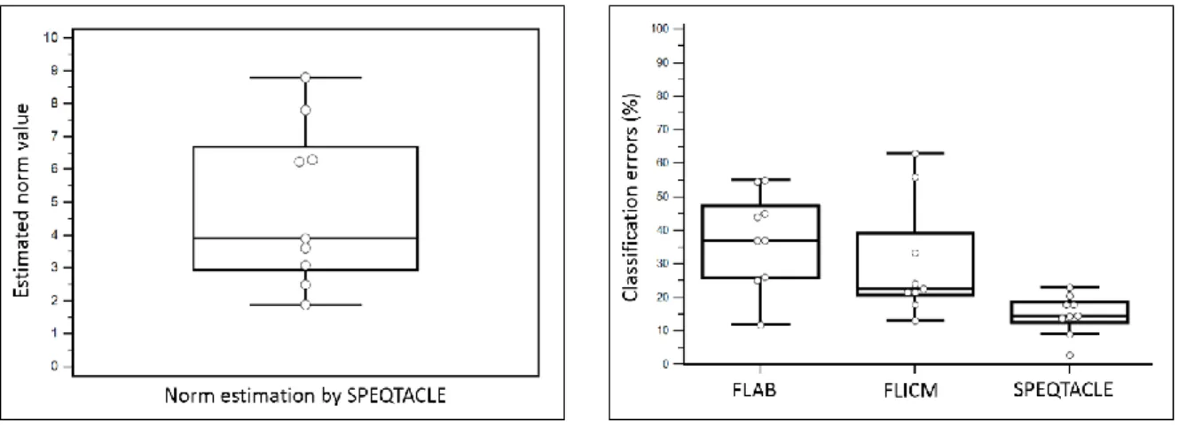
y
p
y
andy
p
(
y
d
)
is given by: 236 I d d
dl ( )* ( ) , where I(
)is the Fisher information matrix and * )(d is the transpose 237
of the vector
d
. 23813 For the generalized Gaussian random variables that we use in SPEQTACLE, the Fisher 239
information relative to the position parameter, the dispersion parameter and the norm 240
parameter are given respectively by: 241
1
1
)
1
(
)
(
I
242 2 ) (
I and
1 1 1 1 1 ) 1 ( 2 1 1 ) ( ' 4 2 3 3 2 I , 243where, and
are the Eulerian function and its log-derivative respectively. In the norm 244estimation algorithm, we evaluate the distance between distributions twice; namely when 245
) ( p
and
( p) are recomputed. It maybe also possible to evaluate the distance when
( p)is 246recomputed.However, if the two other parameter sequences
( p) and
( p) do not vary, one 247can reliably assume that the parameter sequence
( p)does not vary either. As the Fisher 248information relative to is given by ( ) 2
I , for fixed values of and the infinitesimal 249
distance between two generalized Gaussian distributions
p
(
y
,
,
)
and 250)
,
,
(
y
d
p
is
d
and the distance betweenp
(
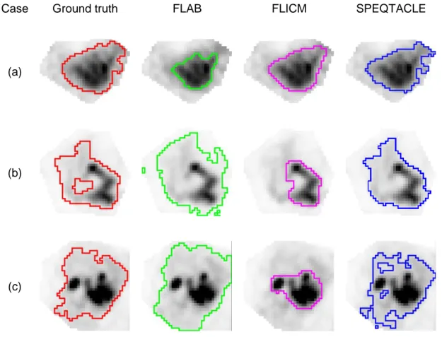
y
,
,
( p))
and 251)
,
,
(
y
(p1)p
is given by: 252
) ( ) 1 ( ) 1 ( ) (log
)
,
(
) 1 ( ) ( p p p p p pd
D
25314 Regarding the parameter , the integration of the Fisher metric is not explicit and requires 254
time consuming numerical methods. We have used the Kullback-information “metric” instead, 255
as a good approximation of the Fisher metric when the consecutive values of
( p) are close 256(Appendix E). When and are set, the Kullback information from
p
(
y
(p),
,
)
to 257)
,
,
(
y
(p1)
p
is given by: 258 ) 1 ( ) 1 ( ) 1 ( ) ( ) 1 ( ) ( ) ( ) 1 ( ) ( ) 1 (1
1
1
1
1
log
)
:
(
p p p p p p p p p pK
. 259Finally, in the maximum likelihood estimation algorithm,
D
(
(p),
(p1))
andK
(
(p1):
(p))
260are evaluated when the value of
(p1)and
(p1)are respectively computed. The stopping 261rule is a fixed threshold value =10-7small enough to ensure convergence. 262
C. Algorithm evaluation methodology 263
Repeatability and dependency of the norm estimation on initial tumor region
264
In order to evaluate the repeatability of SPEQTACLE, the whole process (background-265
subtracted area definition used to estimate the norm, followed by the iterative estimation of 266
the norm and the modified FCM clustering) was applied 20 times to the same tumorimages. 267
In order to investigate the dependency of the estimated norm value on the background-268
subtracted region, we made smaller or larger the result of this fully automated procedure 32 269
by one to three voxels in all directions and relaunched the estimation procedure on the new 270
area. 271
Robustness assessment
272
We firstevaluated the robustness of the SPEQTACLE algorithm. Robustness was defined as 273
the ability of the automatic algorithm to provide consistent results for a given known object of 274
15 interest, considering varying image properties such as spatial sampling (voxel size), SNR, 275
contrast, texture, filtering, etc. This evaluation was carried out using a dataset of phantoms 276
containing homogeneous spheres on homogeneous background that were acquired in 277
different PET/CT scanners, each with varyingacquisition and reconstruction parameters (see 278
section D. Datasets).Homogeneous spheres on homogeneous backgroundare not 279
appropriate for the evaluation of absolute accuracy since they represent a simplisticset-up 280
and because of thebias due to cold sphere walls34, 35. On the other hand, they are well suited 281
for the task of robustness estimationsince any present bias presentis the same for all 282
acquisitions and they can provide a wide range in imaging settings for a given known object. 283
The four spheres with largest diameters (37, 28, 22 and 17 mm) were segmented 284
individually. The 13 and 10mm spheres were not included in the analysis because they were 285
not filled in all acquisitions and are often too small with respect to the reconstructed voxel 286
size to provide meaningfulresults. 287
Accuracy assessment
288
To evaluate the accuracy of the new algorithm relative to that of current state-of-the-art 289
methods more challenging cases such as relatively large, complex-shaped and/or 290
heterogeneous tumors were used considering both simulated realistic tumors and clinical 291
tumor cases (see section D. datasets). 292
Evaluation metrics
293
For the robustness assessment, since the objects used are simple homogeneous spheres 294
and the goal is to assess the consistency of results over various acquisitions of the same 295
object and not absolute accuracy, the standard deviation of the determined volumes for a 296
given sphere across the entire dataset (all scanners, all configurations) was reported as a 297
measure of robustness. 298
For the accuracy evaluation, the classifications errors (CE) were used. In the simulated 299
dataset, CE were calculated relatively to the known ground truth. In the clinical datasets, CE 300
16 were calculated relatively toa surrogate of truth obtained through a statistical consensus 301
using the STAPLE (Simultaneous Truth And Performance Level Estimation) algorithm 36 302
applied to three manual delineations performed by experts with similar training and 303
experience. CE may result from two contributions: the false negatives, the number of 304
misclassified voxels within the ground truth, and the false positives, the number of 305
misclassified voxels outside of the ground truth. CE as a percentage is then calculated as the 306
sum of positive and negative misclassified voxels, divided by the number of voxels defining 307
the ground truth15. CE were reported as mean±SD as well as with box-and-whisker plots in 308
the figures. 309
Comparison with other methods
310
Within this evaluation framework, the proposed algorithm SPEQTACLE was compared to a 311
couple of state-of-the-art methods which are improvement of the classical FCM: the Fuzzy 312
Locally Adaptive Bayesian (FLAB) 16and the Fuzzy Local Information C-means 313
(FLICM)30.Because the standard FCM has already been extensively evaluated and 314
compared to these extensions or other previous segmentation approaches,including on PET 315
images15, 16, 37, it was not included in the present analysis. 316
FLAB combines a fuzzy measure with a Gaussian mixture model, and a stochastic 317
estimation of the parameters from a FCM-based initialization. This method was developed 318
initially for PET and thoroughly validated on both simulated and clinical datasets16, 17, 319
23.FLICM is a recent FCM algorithm with a weighted norm taking into account outliers due to 320
the noise30. This method uses two parameters: a regularization parameter and the size of the 321
surrounding kernel. In the present work, we have set the parameter regularization equal to 1 322
and the kernel radius equal to 3 voxels, which are the recommended values30 although they 323
have not been optimized specifically for PET. 324
For all methods, the object of interest is first isolated in a 3D region of interest (ROI) 325
containing the tumor, similarly as previously detailed for FLAB15. The number of 326
17 classes/clustersused was 2 for the robustness evaluation (homogeneous spheres) and 3 for 327
the accuracy evaluation, in order to take into account potential tumor uptake heterogeneity. 328
The two tumor classes were then unified for the error calculation with respect to the binary 329
ground-truth (tumor/background).Thus, all algorithms were applied considering the same 330
number of classes/clustersfor a given image. 331
The Wilcoxon rank sum testwas used to compare theresults between methods. P-values 332
below 0.05 were considered significant. 333
D. Datasets 334
Homogeneous spheres phantoms
335
The dataset used for the robustness evaluation consists of NEMA phantoms containing 336
spheres of various sizes (37, 28, 22, 17, 13, 10 mm)and filled with 18F-FDG, 337
thatwereacquired in three different PET/CT scanners: two PHILIPS scanners (a standard 338
GEMINI and a time-of-flight (TOF) GEMINI), anda SIEMENSBiograph 16 scanner8. The 339
standard iterative reconstruction algorithms associated with each scanner were used with 340
their usual parameters: Time-of-Flight Maximum Likelihood-Expectation Maximization (TF 341
ML-EM) for the GEMINI TOF, 3D Row Action Maximum Likelihood Algorithm (RAMLA) (2 342
iterations, relaxation parameter 0.05, Gaussian post-filteringwith 5mm FWHM) for the 343
GEMINI, and Fourier rebinning (FORE) followed by Ordered Subsets Expectation 344
Maximization (OSEM) (4 iterations, 8 subsets, Gaussian post-filtering with 5mm FWHM) for 345
the Biograph16. All PET images were reconstructed using CT-based attenuation correction, 346
as well as scatter and random coincidences. For each scanner, two different values for the 347
following acquisition parameters and reconstruction settingswere considered: the contrast 348
between the sphere and the background (4:1 and 8:1), the voxel size in the reconstruction 349
matrix (2×2×2 and 4×4×4 or 5.33×5.33×2 mm3) and the noise level (2 and 5 min of listmode 350
data). Note that for the GEMINI acquisitions, the 28mm sphere was missingin the physical 351
phantom. Figure 1 illustrates the images obtained for some of the acquisitions. 352
18
(a) (b)
(c) (d)
(e) (f)
Fig 1. Examples of phantoms acquisitions: (a-b) the PHILIPS GEMINI TOF scanner with 353
5min acquisitionsand (a) ratio 8:1, voxels 2×2×2 mm3, (b) ratio 4:1, 4×4×4 mm3. (c-d) the 354
SIEMENS scanner with 5min acquisitions and (c) ratio 8:1,voxels 2×2×2 mm3, (d) ratio 4:1, 355
5.33×5.33×2 mm3. (e-f) the PHILIPS GEMINI scanner with ratio 8:1, voxels 4×4×4 mm3, and 356
(e) 5min acquisition, (f) 2 min acquisition. 357
358
Simulated PET images
359
A set of 34 simulated PET tumor images with a wide range of contrast, noise levels, uptake 360
heterogeneity and shape complexity was generated following a previously described 361
methodology to obtain realistic complex shapes and uptake distributions of tumors for which 362
19 the exact ground-truth on a voxel-by-voxel basis is known38, 39. This dataset was built with 363
relatively more challenging cases compared to previously conducted evaluations16, in order 364
to provide more complex tumor cases with combination of low SNR, high levels of 365
heterogeneities and complex shapes. The important steps of the procedure used to generate 366
these images is outlined below, and the reader is referred to38, 39 for more details. 367
Each clinical tumor was first manually delineated on a clinical PET image by a nuclear 368
medicine expert, thus creating a voxelized volume that represents the ground-truth of the 369
tumor model used in the simulation. The activity levels attributed to each of the tumor parts 370
were derived from the activity measured in the same areas of the tumor in the corresponding 371
patient images. This ground-truth tumor structure was subsequently transformed into a Non-372
Uniform Rational B-Splines (NURBS) volume via RhinocerosTM (CADLINK software), for 373
insertion into the NCAT phantom 40attenuation maps at the same approximate position as 374
located in the patient. No respiratory or cardiac motions were considered. Simulations using 375
a model of the Philips PET/CT scanner previously validated with GATE (Geant4 Application 376
for Tomography Emission) 41were carried out. A total of 45 million coincidences were 377
simulated corresponding to the statistics of a clinical acquisition over a single axial 18 cm 378
field of view. Images were subsequently reconstructed using the One-Pass List mode 379
Expectation Maximization (OPL-EM) (7 iterations, 1 subset). In some cases, the same 3D 380
tumor shape was produced with different levels of contrast and heterogeneity, voxel sizes 381
(4×4×4 and2×2×2 mm3) and/or a different number of coincidences (45M or 20M) for different 382
SNR realizations.Figure 2 illustrates some of the simulated tumors. The first two cases (fig. 383
2a-b) present relatively simpler shapes, higher contrast and SNR, whereas fig. 2c and 2d 384
present more complex shapes and higher levels of noise and uptake heterogeneity. 385
20
(a) (b)
(c) (d)
Fig 2. Four examples of simulated tumors. Red contours correspond to the simulation ground 386
truth showing both external contours and sub-volumes heterogeneity. 387
Clinical PET images
388
Nine non-Small Cell Lung Cancer (NSCLC) tumors were chosen for their challenging nature 389
with complex shapes and uptake heterogeneity.Patients fasted for at least 6 hours before 3D 390
PET data was acquired on a Philips GEMINI PET/CT scanner without motion correction, 391
60±4 min after injection of 5MBq/kg of 18F-FDG. Images were reconstructed with the 3D 392
RAMLA algorithm (2 iterations, relaxation parameter 0.05, post-filtering with a Gaussian of 5 393
mm FWHM) and a voxel size of 4×4×4 mm3, using CT-based attenuation correction, scatter 394
and random correction42. In the absence of ground-truth for these volumes, 3 different 395
experts delineated each tumor slice-by-slice with free display settings. A statistical 396
consensus of the segmentations was then derived using the STAPLE algorithm to generate 397
one surrogate of truth (fig. 3). 398
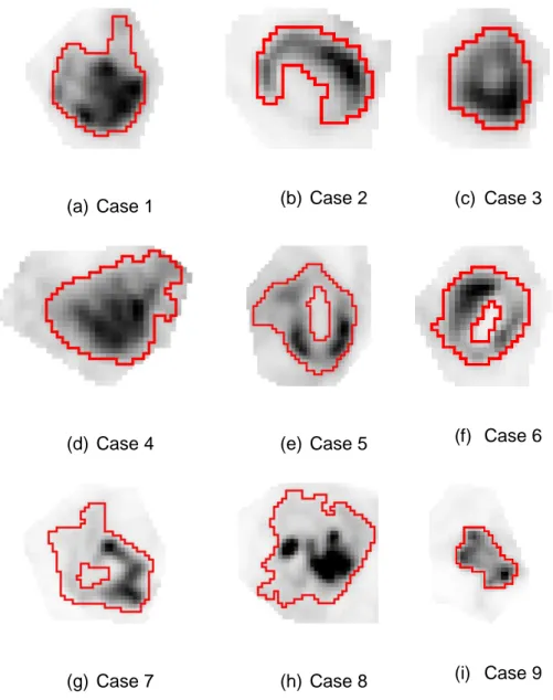
21 (a) Case 1 (b) Case 2 (c) Case 3
(d) Case 4 (e) Case 5 (f) Case 6
(g) Case 7 (h) Case 8 (i) Case 9
Fig 3. (a-i) Clinical images of 9 NSCLC tumors. Red contours correspond to the statistical 399
consensus of 3 different manual delineations. 400
Results
401Repeatability and dependency on initially selected tumor region
402
The procedure was found perfectly repeatable with no variations in the resulting 403
segmentations on repeated applications to the same (previously defined) region of interest. 404
In addition, enlarging or reducing the size of the initial background-subtracted area by 1 to 3 405
voxels in all directions (equivalent to shrinking or increasing of the size of the region used to 406
estimate the norm by 5 to 15%) resulted in only minor variations in the estimated norm value 407
22 (3±11%, range –10% to +16%), and even smaller variations in the resulting segmentation 408
(2±5%, range –4% to +7%). A substantial degradation of the segmentation results (20% 409
difference) was observed when the reduction(area not covering sufficiently the tumor) or 410
enlargement (too much background incorporated) of the initially estimated area exceeded 411
50%. 412
Robustness
413
The robustness of FLAB and standard FCMhas already been reported extensively8. In the 414
current work we focused on three scanners and the 4 largest spheres, comparing 415
SPEQTACLE to FLAB and FLICM.Figure4presents the robustness of each method, 416
quantified bythe distributions of resulting volumes for each sphere as box-and-whisker 417
plotsacross the entire dataset (3 scanners, all acquisition and reconstruction parameters). 418
Although the accuracy was not under evaluation here, the true volume was also plotted for 419
reference. 420
23 Fig 4. Distributions of volumes determined by the three methods under comparison for the 422
four spheres of 37, 28, 22 and 17 mm in diameter across the entire robustness dataset. Box-423
and-whisker plots provide lower to upper quartile (25 to 75 percentile, central box), the 424
median (middle line of the box) and the minimum to the maximum value, excluding "outlier 425
values” which are displayed as separate dots. 426
427
The robustness performance of SPEQTACLE was satisfactory given the very large range of 428
image characteristics. It was very similar and not statistically different (p=0.15) from FLAB 429
with standard deviations of 5.4%, 16.9%, 12.7% and 26.6% for SPEQTACLE vs. 5.4%, 430
11.5%, 20.3%, and 19.3% for FLAB (for the 37, 28, 22 and 17mm spheres respectively). It 431
should be emphasized that there were 2 outliers for the 17mm sphere and 1 for the 22 mm 432
sphere (fig. 4). These were associated with images of some of the acquisitions for which the 433
spheres were barely visible and spatially sampled with large voxels (see fig. 1b for an 434
example), which explains the substantial deviation observed for these specific cases. When 435
excluding these outliers, the robustness of SPEQTACLE increased with lower standard 436
deviations of 7.9% and 18.8% for the 22 and 17mm sphere respectively. 437
FLICM exhibited significantly lower robustness (p<0.0001) than FLAB and SPEQTACLE. For 438
the spheres 28, 22 and 17 mm, this was mostly due to segmentation failures in several cases 439
for sphere diameters ≤28 mm, with the segmentation filling the entire ROI leading to 440
extremely large volumes. For these complete failures, we limited the resulting volume to 441
twice the expected volume of the sphere, leading to standard deviations of 68.9%, 40.9% 442
and 43.7% for the spheres of 28, 22 and 17mm respectively. However for the largest sphere 443
(37 mm in diameter), the standard deviation was also higher (26.8%) than SPEQTACLE and 444
FLAB, without an associated segmentation failure, but rather very different results depending 445
on the different image characteristics considered. 446
24
Accuracy
447
(a) (b)
(c) (d)
Fig. 5 (a) Box-and-whisker plot of the norm parameter estimated by SPEQTACLE for the 448
entire set of simulated PET images. (b-d) Comparison of error rates for the three methods 449
with box-and-whisker plots, for (b) the 34 simulated tumors PET images, (c) the subset of 450
cases with estimated norm<3 and (d) cases with norm>3. 451
Figure5a shows the distribution of the values for the norm parameter as estimated by 452
SPEQTACLE. We recall that a value of 2corresponds to the standard FCM case. Almost half 453
the cases considered had an estimated norm between 3 and 6. Five cases led to estimated 454
norm values of 9 to 19. Given this distribution, we report the accuracy for the entire dataset, 455
then for the subset of cases with norm<3 (15 cases) and finally for >3 (19 cases), as we can 456
25 reasonably expect a larger improvement using SPEQTACLE over the two other algorithms 457
for higher norm values. 458
Figure 5bshows the classification errorsresults obtained by the threemethods under 459
comparison, for the entire set of 34 images.SPEQTACLE was found to provide lower CE 460
than FLAB (p=0.0044) and FLICM (p<0.0001). FLAB, FLICM and SPEQTACLE led to CE of 461
21.8±19.8% (median 14.5%, range 1.2 – 70.2%), 29±29% (median 22.3%, range 3.9 – 462
100.0%) and 14.4±10.6% (median 12.5%, range 1.3 – 37.9%)respectively. No errorsabove 463
40% were observed for SPEQTACLE contrary to FLAB (up to 50-70% errors) and FLICM 464
that even had four cases with >100% errors (complete failure of the segmentation, CE limited 465
to 100%). SPEQTACLE had more cases with errors below 10% and between 10% and 20% 466
than FLAB and FLICM, and fewer cases with errors between 20% and 50%. 467
Figure 5c provides the classification errors for the 15 images for which the estimated norm 468
was <3.In this first subset, although SPEQTACLE led to the best results (10.5±8.5%, median 469
8.3%, range 1.3 – 31%) with significantly lower errors than FLICM (15.3±9.1%, median 470
12.9%, range 4.2 – 34.8%, p=0.0215), no significant differences were found between 471
SPEQTACLE and FLAB (14.5±13.6%, median 9.5%, range 1.2 – 46.1%, p=0.22). No errors 472
above 50% were observed for any method.It should be emphasized that despite differences 473
between the three methods, all three achieved high accuracy performance with <20% CE for 474
the majority of cases. 475
Figure 5dprovides the classification errors for the second subset of 19 images for which the 476
estimated norm was >3.In this dataset of clearly more challenging cases, with an error rate of 477
17.4±11.3% (median 21%, range 1.4 – 37.9%), SPEQTACLE significantly outperformed all 478
other methods:FLAB with 27.6±22.2% (median 22.2%, range 1.4 – 70.2%) (p=0.0092) and 479
FLICM with 39.9±34.6% (median 30.5%, range 3.9 – 100.0%) (p<0.0001).No errors above 480
50% were observed for SPEQTACLE contrary to FLAB and FLICM, and there were less 481
errors between 20 and 50% for SPEQTACLE than for FLAB and FLICM. Overall, the 482
26 accuracy achieved by SPEQTACLE in this dataset of very challenging cases was 483
satisfactory, with a maximum CE below 38% and a mean of17%. Figure 6 provides some 484
visual examples of segmentation results for the simulated tumors. 485
Ground-truth
Norm=4 Norm=5 Norm=10 Norm = 18.5
FLAB
CE=35% CE=28% CE=46% CE=37%
FLICM
CE=25% CE=25% CE=29% CE=40%
SPEQTACLE
CE=22% CE=17% CE=23% CE=30%
27 Fig 6. Segmentation results for (a-c) the same simulated tumor with increasing complexity: 486
combinations of noise levels and heterogeneity both within the tumor (contrast between the 487
various sub-volumes of the tumor) or in terms of overall contrast between the tumor and the 488
background. These configurations were found to correspond to increasing estimated norm 489
values: (a) 4, (b) 5 and (c) 10. (d)presents a tumor with complex shape and high levels of 490
heterogeneity for which the norm was estimated at 18.45. First row is ground-truth (red) 491
whereas second, third and fourth rows are results from FLAB (green), FLICM (magenta) and 492
SPEQTACLE (blue). 493
Figure 7shows the estimated norm values (fig. 7a) and the classification errors(fig. 7b) for the 494
nine clinical images.Norm values estimated by SPEQTACLE were between 2 and 9, with 495
most of them being >3 (7 out of 9 cases). The best performance was obtained with 496
SPEQTACLE with significantly (p<0.004) lower errors (mean 14.9±6.1%, range 2.9 – 23%) 497
with respect to the STAPLE-derived consensus of manual delineations, compared to FLAB 498
(mean 37.3±14.3%, range 12 – 55%) and FLICM (30.4±17.4%, range 13.2 – 63%). 499
(a) (b)
Fig 7. (a) Box-and-whisker plot of the norm parameter estimated by SPEQTACLE and (b) CE 500
for the three methods, for the clinical dataset. 501
Figure 8 shows the results of segmentation for all 9 clinical cases.For cases 3 and 9, the 502
three methods led to similar results, as the level of heterogeneity is relatively lower with 503
28 respect to the high overall contrast between the tumor and the surrounding background. On 504
the one hand, for cases 1, 4, 5 and 6, it was observed that FLAB underestimated the spatial 505
extent selected by the experts, by focusing on the high intensity uptake region, whereas 506
FLICM led to results closer to the manual contours. On the other hand, for cases 2, 7 and 8, 507
on the contrary FLAB slightly overestimated the manual contours, whereas FLICM 508
underestimated it, missing the large areas with lower uptake. In all cases, SPEQTACLE 509
demonstrated higheraccuracywith results closer to the manual delineations. 510
Case Ground truth FLAB FLICM SPEQTACLE
(a)
(b)
(c)
Fig 8. Examples of delineationsfor clinical cases (a) 4, (b) 7 and (c) 8 from Fig. 3 (d), (g) and 511
(h): consensus of manual (red), FLAB (green), FLICM (magenta) and SPEQTACLE (blue). 512
Discussion
513Although promising results for PET tumor delineation in a realistic setting beyond the 514
validation using simple cases (spherical and/or homogeneous uptakes)have been recently 515
achieved by several methods11there is still room for improvement, particularly in the case of 516
29 highly heterogeneous and complexshapes.The use of the fuzzy C-means clustering 517
algorithm for delineation of PET tumors has been considered previouslyshowing a limited 518
performance both in accuracy 15, 43, 44and robustness8. Among the recent methods dedicated 519
to PET that demonstrated promising accuracy, the fuzzy C-means algorithm was improved 520
using a rather complex pipelinecombining spatial correlation modeling and pre-processing in 521
the wavelet domain 44. In the presented work, we rather focused on the generalization and 522
full automation of the FCM approach to improve its accuracy and its ability to deal with 523
challenging and complex PET tumor images, by implementing an estimation of the norm on a 524
case-by-case basis. The improved accuracy results that we obtained on the validation 525
datasets suggest that the optimal norm parameter can indeed be different for each PET 526
tumor image and can vary substantially across cases, making anautomatic estimation 527
essential in the accuracy of the FCM segmentation results. 528
It should be emphasized that SPEQTACLE did not undergo any processing or pre-529
optimization and that no parameter was set or chosen to optimize the obtained results on the 530
evaluation datasets (either phantoms, realistic simulated or clinical tumors).The improved 531
accuracy that SPEQTACLE achieved is thereforeentirely due to its automatic estimation 532
framework and its associated ability to adapt its norm parameter to varying properties of the 533
image. The advantage of SPEQTACLE compared to other fuzzy clustering-based methods 534
such as FLAB or FLICM thus lies on its ability to estimate reliably the norm parameter value 535
on a case-by-case basis. In addition, the proposed norm estimation scheme is deterministic 536
and convergent, therefore the repeatability of the algorithm was found to be perfect with zero 537
variability in the results on repeated segmentations of the same image, which is an important 538
point to ensure clinical acceptance for use by the physicians. In addition, the estimation of 539
the norm was also found to be robust with respect to slightly larger or smaller initial 540
determination of the tumor class using a background-subtraction approach32. In order to 541
reach substantial differences in the segmentation results, this area had to be enlarged or 542
30 shrunk by more than 50%, which is very unlikely to occurunless highly inaccurate methods 543
are used to define the initial region. 544
We showed that SPEQTACLE led to significantlyhigher accuracyin delineating tumor 545
volumes with higher complexity (either in terms of shape, heterogeneity, noise levels and/or 546
contrast), associated with a norm value higher than 3, on both simulated and clinical 547
datasets. On the other hand, for simpler objects of interest (norm value below 3), we found 548
that SPEQTACLE provided similar (although slightly improved) accuracy as FLAB and 549
FLICM.Given the improved accuracy obtained with respect to FLAB on a dataset with a large 550
range of contrast and noise levels as well as heterogeneity and shape, we expected that the 551
robustness of SPEQTACLE should be at least similar as the one of FLAB. We indeed 552
confirmed through a robustness analysis that the proposed automatic norm estimation 553
scheme does not lead to decreased robustness with respect to varying image properties 554
associated with the use of different PET/CT scanner models, reconstruction algorithms, or 555
acquisition and reconstruction settings. Indeed, the level of robustness exhibited by 556
SPEQTACLE was found to be similar to the one of FLAB, which had already been 557
demonstrated as substantially more robust than standard FCM8. FLICM however was found 558
to be much less robust, with segmentation failures for some of the configurations in the 559
dataset. Given the fact that FLICM performed reasonably well on the accuracy dataset, its 560
failure on the robustness evaluationmight be due to the two parameters (the regularization 561
parameter and the size of the surrounding kernel) that were set a priori in this study using 562
recommended values that might not be appropriate for some of the PET images of the 563
robustness dataset. The overall performance of FLICM might therefore be improved by 564
optimizing these two parameters for each phantom acquisition, which is however out of the 565
scope of the present work. 566
From a clinical point of view, our method might be easier than most of the previously 567
proposed onesto implement in a clinical setting because it is fully automatic and perfectly 568
repeatable, with no user intervention for parameterization beyond the localization of the 569
31 tumor in the whole-body image and its isolation in a 3D ROI. It is also very fast due to its low 570
computational cost; thesegmentation of thelargest tumor (55×55×25 voxels) requires less 571
than 1 min on a standard computer (CPU E5520 2.27 GHz×8), which could be easily 572
shortened through algorithmic optimization and parallel computing or GPU implementation. 573
Moreover, the algorithm itselfuses a negligible amount of memory. 574
The present work has a few limitations. It should be reminded that the proposed algorithm 575
aims at the accurate delineation of a single pathological uptake previously detected and 576
isolated in a ROI, similarly as FLAB. It was therefore not evaluated within the context of the 577
simultaneous segmentation of multiple tumors (as each tumor should be processed 578
independently when using SPEQTACLE), the detection of tumors and/or lymph nodes in a 579
whole-body image45, nor the segmentation of diffuse and multifocal uptakes such as in 580
pulmonary infection46. Also, we did not investigate the impact on the resulting segmentation 581
of theinitial ROI selection, which is a first step as in most of published methods for PET tumor 582
delineation10, 11. However, we already showed that this step has a very limited impact on the 583
results for FLAB, as long as the ROI selection is made without incorporating nearby non-584
relevant uptake that would bias the estimation process15. Given that SPEQTACLE 585
demonstrated similar robustness as FLAB, the impact of this step should be similarly low. 586
Second, we did not include a large number of methods to compare SPEQTACLE with. Given 587
its previous validation and demonstrated performance, FLAB can be considered a state-of-588
the-art method and our primary goal was to improve on that approach for challenging cases. 589
A full comparison with numerous other methods was out of the scope of this work and might 590
be conducted in the future using the benchmark currently being developed by the AAPM 591
taskgroup 211147. Second, the robustness analysis was carried out on a smaller dataset than 592
for the previously reported analysis for FLAB, FCM and thresholding methods8, however the 593
dataset is certainly representative enough to provide a clear picture. Third, we did not 594
evaluate the algorithms on clinical datasets with histopathology associated measurements. 595
1
32 The one dataset available to us consists of maximum diameter measurements only17, which 596
might not be sufficient to highlight differences between the advanced algorithms under 597
comparison. On the other hand, a benchmark developed by the AAPM Taskgroup 211 is 598
expected to contain several clinical datasets with histopathological volumes47, and could be 599
used for future comparison studies. Finally, in the present implementation, the norm 600
parameter was estimated from an automatically pre-segmented estimation of the tumor 601
region, using a background-subtraction approach 32 in order to obtain a first guess of the 602
tumor class. The estimated norm was then used for all classes in the segmentation.In future 603
work, it would therefore be possible topotentially improve the algorithm performanceby 604
estimating a norm parameter for each class in the ROI. In this case, the minimized criterion 605 in GFCM becomes: 606
V u C i i u m i u iy
p
1 ,
. 607The norm parameter icannot be estimated by using the Newton-Raphson algorithm on the
608
minimized criterion of equation (4). Indeed, the norm parameter is essentially dependent on 609
the statistical behavior of the data and generally there is no solution
i
1
which minimizes 610equation (4). Thus minimizing equation (4) according to i is equivalent to solving:
611
0
log
1 ,
V u C i i u i u m i u iy
y
p
. 612Consequently, it depends on how data are scaled and the presence of
y
u such that 6131
iu
y
contributes to making this derivative > 0. Amongst other possible extensions, it 614will be interesting to estimate a variance parameter additionally to the center parameter
i615
and the norm parameter. Such a method would be able to fit more completely the statistical 616
distribution of the intensities. Indeed,
i controls the mean of intensities for each cluster, i 617controls the shape of the distribution whereas the variance parameter controls the disparity 618