HAL Id: inserm-00333460
https://www.hal.inserm.fr/inserm-00333460
Submitted on 23 Oct 2008
HAL is a multi-disciplinary open access
archive for the deposit and dissemination of
sci-entific research documents, whether they are
pub-lished or not. The documents may come from
teaching and research institutions in France or
abroad, or from public or private research centers.
L’archive ouverte pluridisciplinaire HAL, est
destinée au dépôt et à la diffusion de documents
scientifiques de niveau recherche, publiés ou non,
émanant des établissements d’enseignement et de
recherche français ou étrangers, des laboratoires
publics ou privés.
probable AD versus normal controls.
Simon Duchesne, Anna Caroli, Cristina Geroldi, Christian Barillot, Giovanni
Frisoni, Louis Collins
To cite this version:
Simon Duchesne, Anna Caroli, Cristina Geroldi, Christian Barillot, Giovanni Frisoni, et al..
MRI-based automated computer classification of probable AD versus normal controls.. IEEE
Transac-tions on Medical Imaging, Institute of Electrical and Electronics Engineers, 2008, 27 (4), pp.509-20.
�10.1109/TMI.2007.908685�. �inserm-00333460�
MRI-Based Automated Computer Classification of
Probable AD Versus Normal Controls
Simon Duchesne*, Member, IEEE, Anna Caroli, C. Geroldi, Christian Barillot, Senior Member, IEEE,
Giovanni B. Frisoni, and D. Louis Collins
Abstract—Automated computer classification (ACC) techniques
are needed to facilitate physician’s diagnosis of complex diseases in individual patients. We provide an example of ACC using compu-tational techniques within the context of cross-sectional analysis of magnetic resonance images (MRI) in neurodegenerative diseases, namely Alzheimer’s dementia (AD). In this paper, the accuracy of our ACC methodology is assessed when presented with real life, imperfect data, i.e., cohorts of MRI with varying acquisition pa-rameters and imaging quality. The comparative methodology uses the Jacobian determinants derived from dense deformation fields and scaled grey-level intensity from a selected volume of interest centered on the medial temporal lobe. The ACC performance is assessed in a series of leave-one-out experiments aimed at sepa-rating 75 probable AD and 75 age-matched normal controls. The resulting accuracy is 92% using a support vector machine classi-fier based on least squares optimization. Finally, it is shown in the Appendix that determinants and scaled grey-level intensity are ap-preciably more robust to varying parameters in validation studies using simulated data, when compared to raw intensities or grey/ white matter volumes. The ability of cross-sectional MRI at de-tecting probable AD with high accuracy could have profound im-plications in the management of suspected AD candidates.
Index Terms—Accuracy, automated computer classification,
magnetic resonance imaging (MRI), neurodegenerative diseases.
I. INTRODUCTION
N
EURODEGENERATIVE diseases can be characterized by their gradual modification of the cellular environment leading to neuronal dysfunction, abnormal loss of brain tissue, and accompanying cognitive impairment. The factors and mechanisms underlying these processes will vary from one disease to another. In Alzheimer’s disease (AD), abnormal accumulation of insoluble A and Tau proteins into intra- and extra-cellular formations has been linked to cerebral tissue damage, leading to dementia [1]. The pattern of distribution of plaques and tangles has been characterized by Braak et al. [1] in six neuropathological stages, ranging from initial deposition in the medial temporal lobe to distribution throughout theManuscript received June 22, 2007; revised September 10, 2007. The work of S. Duchesne was supported by the FRSQ/INSERM. Asterisk indicates
cor-responding author.
*S. Duchesne is with the Centre de Recherche de l’Université Laval Robert Giffard, Québec, QC, G1J 2G3 Canada (e-mail: [email protected]).
A. Caroli, C. Geroldi, and G. Frisoni are with Neuroimaging and Telemedicine (LENITEM), IRCCS San Giovanni di Dio, Fatebene-fratelli, 25125 Brescia, Italy (e-mail: [email protected]; cgeroldi@ fatebenefratelli.it; [email protected]).
C. Barillot is with the Unite U746/Equipe VISAGES, IRISA, 35043 Rennes, France (e-mail: [email protected]).
D. L. Collins is with the Brain Imaging Center, McGill University, Montreal, QC, H3A 2T5 Canada (e-mail: [email protected]).
Digital Object Identifier 10.1109/TMI.2007.908685
cortex. This etiology implies that final AD diagnosis can only be confirmed at present by postmortem histopathological as-sessment. Structural images, such as T1, T2, and PD weighted magnetic resonance imaging (MRI) sequences acquired on standard clinical scanners of 1.0–3.0 T field strength, lack the resolution to measure directly microscopic changes due to probable AD in the cellular environment. Thus, it is clear that structural imaging cannot be used for deriving a final diagnosis; it can, however, image some of the resulting macroscopic disease-related effects that result in changes in shape, size, or image intensity of anatomical structures [2]. Specifically, the role of structural imaging in probable AD has shifted from one of exclusion of other possible causes of dementia to one of
in vivo disease-specific marker that, it is hoped, can identify the
disease at a very early stage [3], [4].
Various computer-aided techniques have been proposed in the past and include the study of texture changes in signal in-tensity [5], grey matter (GM) concentrations differences [6], atrophy of subcortical limbic structures [7]–[9], and general cor-tical atrophy [10]–[12]. These automated studies typically re-port group-level differences between probable AD patients and age-matched control subjects for various brain structures [2], often in a longitudinal setting.
The goal of our research into automated computer classifi-cation (ACC) techniques is to achieve individual classificlassifi-cation. Further, we restrict our focus to cross-sectional or single time point assessment, as opposed to longitudinal acquisitions, since the former allows for a more timely alteration in therapy course that may represent a significant advantage when dealing with neurodegenerative diseases.
Within this context, the standard in terms of image analysis in probable AD remains manual segmentation of specific struc-tures such as the hippocampus (HC) and parahippocampal gyrus (PHG). HC and PHG volumetric measurements have achieved individual classification rates between controls and probable AD patients as high as 93% when using linear combinations of volumes [13], [14]. Manual segmentation however is a time-consuming, center and expert-dependent technique [15], [16] that cannot be used in regular clinical practice.
ACC techniques on the other hand can be objective, quanti-tative, and practical. Previous reports on ACC mention the use of a variety of image features to fulfill the task of individual classification. The signal intensity was modeled, either directly [17], via texture analysis [5], [18], or via GM tissue classifi-cation [19]; classificlassifi-cation based on the morphometry of specific brain structures has been proposed [9], [20], [21]; and lately cor-tical mantle thickness estimates have been investigated [12]. For these methods, the robustness to varying scanning parameters, repetition/echo time (TR/TE), field inhomogeneity and noise has yet to be studied and/or reported. The strength of any ACC
system should not lie solely in the optimality of its classifier but also in its choice of features; they must be representative of the disease process, and robust, that is, capable of providing the same information irrespective of noise, artifact, or intrinsic vari-ation in the underlying image due to different parameter settings [22]. Real life datasets are rife with such differences. Sources of errors in MRI measurements have been aptly described and doc-umented exhaustively elsewhere [23], and include, but are not limited to
• signal noise;
• intensity nonuniformity (INU);
• parameter changes (small changes in TR/TE); • voxel dimension changes;
• missing slices; • anatomical variability.
This assumes that all subjects to be assessed have been scanned on the same system, whose configuration (hardware, software) remained stable over time. It is important to note that there are no issues of scan–rescan effects for cross-sectional analysis, such as repositioning, as might be the case in longitu-dinal data [24], [25].
Our original contribution in ACC design is the combination of intensity and local shape descriptor [17] extracted from a large volume of interest (VOI), avoiding the pitfalls of structure segmentation and modeling de facto neighboring tissue interac-tions. Thus, the ACC assessment is based on estimating the indi-vidual subject’s propensity at exhibiting pathology-specific pat-terns of covarying tissue changes within the VOI; these can be expressed as areas of signal changes or tissue atrophy [17], [26] and related to biological phenomena. This is in line with recent findings in aging and probable AD [27]–[29]. It must be empha-sized that we are not claiming to detect molecular changes per se on standard field strength MRI; rather, we are interested in detecting macroscopic pathology-related changes. Equally im-portant is the fact that the VOI selected for this study is centered on the medial temporal lobes, as it represents the area most af-fected in probable AD; it does not address whole brain changes. This VOI is suitable for the classification of probable AD versus normal controls, but may not be appropriate for other classifica-tion tasks.
In this paper, our goal is to evaluate the robustness of our ACC methodology for probable AD versus controls differentiation [30] when presented with random and systematic errors in real and simulated datasets, such as changes in the acquisition pa-rameters and varying INU. Our hypothesis is that the accuracy
of our methodology will not be affected by realistic variations in the acquisition parameters. The focus is therefore on finding a
workable solution to the problem of unequal scan quality found in a day-to-day clinical operation. This is a necessary first step before assessing the accuracy of our ACC methodology in mul-tisite/multiscanner situations, itself a requirement before using such techniques in routine clinical use. These scenarios are out-side the scope of this paper.
II. METHODS
A. Subjects
A total of 299 subjects were included in this study. The first cohort, or reference group, consisted in 149 young, neurolog-ically healthy individuals from the International Consortium for Brain Mapping database (ICBM) [31], whose scans were
used to create the nonpathological, reference space. The second cohort, or study group, consisted in 150 subjects: 75 patients with a diagnosis of probable AD and 75 age-matched normal controls (NC) without neurological or neuropsychological deficit. The AD subjects are individuals with mild to moderate probable AD [32] recruited among outpatients seen at the Centro San Giovanni di Dio Fatebenefratelli, The National Center for AD (Brescia, Italy) between November 2002 and January 2005. History was taken with a structured interview from a knowledgeable informant (usually the patient’s spouse) and was particularly focused on those symptoms that might help in the differential diagnosis of the dementias in order to avoid contamination of non-AD dementias in the study group. Laboratory examinations included complete blood count, chemistry profile, thyroid function, B12 and folic acid, and EKG. A neurologist performed structured neurological examination and a geriatrician performed the physical exami-nation. A comprehensive neuropsychological battery was also administered. The MRIs were not used in the assessment of the subject’s condition. NC subjects were taken from an ongoing study of the structural features of normal aging. This study recruits outpatients attending the Neuroradiology Unit of the Citta’ di Brescia Hospital (Brescia, Italy) aged 40 and older and undergoing brain magnetic resonance (MR) scan for reasons other than cognitive impairment (usually headache and vertigo) and negative for major stroke, tumor, aneurysm, or other focal lesions. Incidental atrophy, white matter disease, and lacunes were not exclusionary criteria. Normality of cognitive functions was ascertained through neuropsychological evaluation and structured interview. Analysis of hippocampal shape for some of these probable AD and NC subjects has been published elsewhere [8].
The Ethics Committee of the IRCCS San Giovanni di Dio FBF (Brescia, Italy) approved the study and informed consent was obtained from all participants.
B. Images
The ICBM subjects from the reference group were scanned in Montreal, QC, Canada on a Philips Gyroscan 1.5-T scanner (Best, The Netherlands) using a T1-weighted fast gradient echo sequence (sagittal acquisition, ms,
ms, 1 mm 1 mm 1 mm voxels, flip angle 30 ), for all acquisitions.
MRI data for all subjects in the probable AD and NC study group were acquired in Brescia, Italy on a single Philips Gyroscan 1.0-T scanner (Best, The Netherlands) using a T1-weighted fast field echo sequence (sagittal acquisition). As the protocol set general guidelines for study parameters, there exist three combination of repetition and echo times (TR/TE) for both NC and probable AD groups, as described in Table I. Albeit the differences are small, the resulting images have slightly different contrasts between GM, white matter (WM), scalp tissue, and fat. Even though specified at 1.0 mm 1.0 mm, there also co-exists small variations in the in-plane resolutions. While the slice thickness remained equal (1.3 mm), the in-plane pixel size ranged from slightly below (0.9 mm 0.9 mm) to slightly above (1.1 mm 1.1 mm) the requirement. The distribution of in-plane resolution parameters
TABLE I
ACQUISITIONPARAMETERGROUPDISTRIBUTION
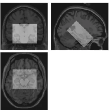
Fig. 1. Coronal, sagittal, and transverse views through the Colin27 high-reso-lution target with the 405 000 voxel VOI (superimposed in white), centered on the medial temporal lobe.
was approximately similar in either probable AD (34 below, 22 standard, 19 above; respectively, 45.3%, 29.3%, and 25.3% of total) or NC groups (41 below, 19 standard, 15 above; respec-tively, 54.7%, 25.3%, and 20% of total).
The use of a common referential target (from hereon, called the “target”) allows for interindividual comparisons. Rather than using a population average, we used a high-contrast, high-res-olution target consisting in the average of 27 T1w MRI scans of the same individual [33], known as the Colin27 MRI average (see Fig. 1). This target exists within a Talairach-like stereotaxic space defined in the context of the ICBM project. Acquisition of the target images was done on the same scanner as the ICBM or reference dataset, using an identical acquisition protocol.
C. Image Processing
All volumes (reference and study subjects, phantoms) were processed according to a similar pipeline, schematized in Fig. 2. The first step following image reconstruction (Fig. 2, item 1) consisted in the correction of the impact of INU (Fig. 2, item 2) due to scanner variations on global MRI data using a non-parametric estimation of the slow varying nonuniformity field [34] (Fig. 2, item 3). Next, prior to spatial alignment of the individual image with the target volume, we scaled its mean
volume intensity to the target mean intensity and fixed the inten-sities within a [0–100] range (Fig. 2, item 1). Spatial alignment of individual images to the target volume (Fig. 2, item 1) was performed using a multistep procedure comparing intensity in-formation from the slightly blurred subject image (FWHM mm ) to the unblurred target [35], increasing at each step the number of degrees of freedom (DF) from a rigid to affine esti-mate (6, 7, 9, then 12 DF). Due to the difference in sequence parameters, the problem was treated as one of multimodality matching, and, therefore, mutual information was chosen as the objective cost function [36], [37]. This choice of cost function also has the advantage of reducing the impact of any intensity difference due to the parameters under study (e.g., TR/TE, INU, noise). This linear registration process was repeated twice, once (Fig. 2, item 5) to optimize the global brain orientation and size, and a second time (Fig. 2, item 6) to optimize the local align-ment of the volume of interest (VOI) from the subject’s brain (Fig. 2, item 8) to the corresponding target VOI. The single VOI selected for this study encompassed both medial temporal lobes, and was oriented towards the long axis of the hippocampus (see Fig. 1). It measured voxels. De-fined within the Colin27 target space, its extent captured the hip-pocampus and neighboring limbic structures (e.g., amygdala, parahippocampal gyrus), irrespective of normal interindividual variability. As a part of the alignment procedure, the data were resampled (Fig. 2, item 7) using trilinear interpolation onto a 1-mm isotropic grid [35]. The first feature of our model con-sists in the rasterized, resampled, scaled grey-level data from the linearly registered VOI, denoted (Fig. 2, item 10).
Nonlinear image registration (Fig. 2, item 9) was then per-formed to derive our shape estimator of local volume change, the second central feature of our ACC methodology. Nonlinear reg-istration attempts to match image features from a subject volume to those of the target image at a local level, typically in a hier-archical fashion, with the aim of reducing a specific cost func-tion. Whereas many nonlinear registration processes exist, the one chosen for this study was ANIMAL [35]. This algorithm attempts to match image grey-level intensity features at a local level (voxel) in successive blurring steps, by maximizing the mutual information of voxel intensities between the subject and target images. The result is a dense deformation field capturing the displacements required to align all voxels within the subject VOI with those of the target VOI. Our local volume change esti-mate is computed (Fig. 2, item 11) from the determinants of the Jacobian of the deformation fields. Our implementation of de-terminant follows the notation developed by Chung et al. [38]. If is the displacement field which matches homologous points between two images, then the local volume change of the defor-mation in the neighborhood of any given voxel is determined by the Jacobian [38], which is defined as
(1)
where denotes the identity matrix and is the 3 3 displacement gradient matrix of .
The rasterized determinant det , denoted d, is the second feature of our model (Fig. 2, item 11). It represents a biologically meaningful quantity, as it is an indicative measure of local brain
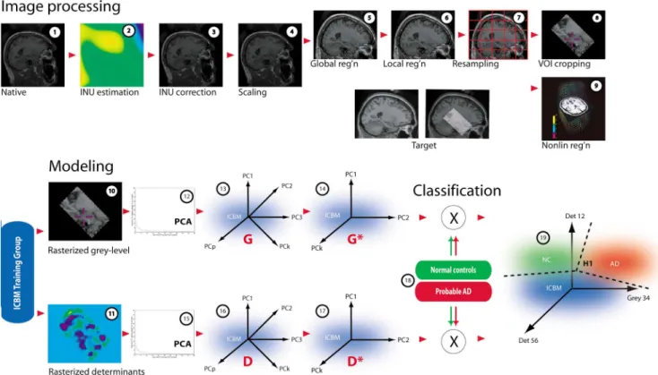
Fig. 2. Schematic representation of the automated computer classification methodology. Images (1) from all subjects are processed in an identical fashion, which includes intensity non uniformity correction (2–3), scaling (4), global and linear registration (5–7), volume of interest extraction (8, 10), nonlinear registration and computation of determinants from the Jacobian of the deformation field (9,11). Principal components analysis is used to reduce the dimensionality of the data and build a model of grey-level intensity (12–14) and determinant eigenvectors from images of 149 healthy young subjects from the ICBM reference group (15–17). Image data from the study cohort (75 probable AD patients, 75 age-matched normal controls) are projected within this reference eigenspace (18). Classification is achieved by calculating the hyperplane or hypersurface separating both groups using either discriminant analysis or SVMs (19). Coronal, sagittal, and transverse views through the Colin27 high-resolution target with the 405 000 VOI ( superimposed in white), centered on the medial temporal lobe.
tissue volume difference when compared to the target volume. When the change is near zero in the neighborhood of , there is no local difference in volume between subject and target im-ages. However, if the determinant is positive, the volume in-creases whereas when negative, the volume dein-creases after the deformation.
D. Modeling and Classification
Our classification approach has been to create a model eigenspace based on grey-level intensity g and determinant information d from subjects in the ICBM database, the co-ordinate space in which we projected image data from our cohorts of patients. The classification was then based on the eigencoordinate distributions of the projected data.
Principal components analysis (PCA) (Fig. 2, items 12 and 13) is used to reduce the dimensionality of the input reference data and generate a linear variation model of covarying infor-mation for the ICBM subjects. A more thorough description of the PCA process was presented in a previous publication [17], based on the seminal work of Cootes and Taylor [39]. In short, we use as input data rasterized vectors of intensity g and Ja-cobian determinants d for all images i belonging to the ICBM reference dataset . Whereas a space built from young, neurologically healthy individuals may not be optimal to represent the study group, our primary goal was to create an independent basis for a comparative evaluation of the MRIs from probable AD and NC individuals and their subsequent
in-dividual classification, rather than a descriptive space that would be the best mathematical representation for aging and disease.
To make the PCA a zero-mean process modeling differences between subjects and the group mean, we first substract the re-spective grey-level and determinant averages of the ICBM ref-erence groups from each input vector
(2) (3) To define the model, PCA is applied to the 149 and 149 ref-erence input data vectors (see Cootes et al. [39] and Duchesne
et al. [17], [40] for a more thorough description of the PCA
process). The resulting ensemble of principal components, where , defines an allowable grey-level domain (Fig. 2, item 14) and allowable determinant domain (Fig. 2, item 15) as the spaces of all possible elements expressed by the determinant eigenvectors and .
Most of the variation can usually be explained by a smaller number of modes, , where and . The total variance of all the variables is equal to
(4)
whereas for eigenvectors, explaining a sufficiently large pro-portion of , the sum of their variances, or how much these prin-cipal directions contribute in the description of the total variance
of the system, is calculated with the ratio of relative importance of the eigenvalue associated with the eigenvector
(5)
The theoretical upper-bound on the dimensionality f of G and D is however, we define restricted versions of these spaces denoted and (Fig. 2, items 16 and 17), using only the first eigenvectors corresponding to a given ratio for each space.
Following the notation of Duda et al. [41], we have defined two states of nature for our study subjects: , and probable AD. For the purposes of this work, the prior probabilities , were known equal
since the compositions of the classification data sets were determined. It must be stated that they do not repre-sent the normal incidence rates of probable AD in the general population.
Once the model eigenspaces and from reference data have been formed, we proceed with the task of projecting the rasterized vectors i and d for the subjects in the study group (Fig. 2, item 18). The projected data in the Domain G* forms the eigencoordinate vectors ; likewise, projected data into the Domain forms the eigencoordinate vectors .
The distribution of eigencoordinates along any principal component for a given population is assumed normally dis-tributed; this normality was assessed via quantile plots and Shapiro-Wilke statistics. Under this assumption of normality, we can use the vectors and as feature vectors in a system of supervised linear classifiers (Fig. 2, item 19). The -dimen-sional real vectors and are normalized to guard against variables with larger variance that might otherwise dominate the classification.
For the purposes of this study we wanted to test simple yet robust classifiers, namely the following.
1) Linear and quadratic discriminant analyses (LDA, QDA). Both are used in machine learning to separate measure-ments of two or more classes of objects or events by either a linear or a quadric surface. In QDA there is no assumption that the covariance of each of the classes is identical. Forward stepwise analysis using Wilk’s method with two different values of (0, 005; 0,01) was used to select the discriminating variables. Classification experiments were computed using the MATLAB Statistics Toolbox (The MathWorks, Natick, MA). The different parameter combinations are detailed in Table II.
2) Support vector machines (SVM). SVMs are a class of linear classifiers that attempt to achieve maximum separa-tion (margin) between the two classes [42]. Experiments were run using three kernels (linear, quadratic, or poly-nomial of third degree), two optimization techniques [two-norm, soft margin (SM) and least squares (LS)], and different constraint sizes on the margin (bounding box). Classification experiments were performed using the MATLAB Statistics Toolbox. The different parameter combinations are detailed in Table II.
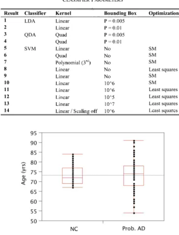
TABLE II CLASSIFIERPARAMETERS
Fig. 3. Study group age distribution.
All classification experiments were run as leave one out trials. In this subset of cross-validation approaches, one subject is re-moved at a time from the study group; the remaining subjects are used as training data to estimate the classification function. The subject left out is then classified independently from the training group. The process is repeated times, being the number of subjects in the study group . The leave-one-out cross-validation has been shown to give an al-most unbiased estimator of the generalization properties of sta-tistical models [43]. The leave-one-out experiments were per-formed using MATLAB’s Statistics Toolbox.
Results were obtained in terms of accuracy (proportion of all subjects correctly classified), sensitivity (proportion of individ-uals with a true positive result), specificity (proportion of in-dividuals with a true negative result), positive predictive value (PPV) (true positive over all positive results), and negative pre-dictive value (NPV) (true negative over all negative results).
Four sets of experiments were conducted.
1) NC versus probable AD classification using linear
discrim-inant analyses. Experiment 1 (LDA) was designed to
as-sess the accuracy of individual classification using forward, stepwise linear discriminant leave-one-out analyses. 2) NC versus probable AD classification using quadratic
dis-criminant analyses. Experiment 2 (QDA) was designed
to assess the accuracy of individual classification using forward, stepwise quadratic discriminant leave-one-out analyses.
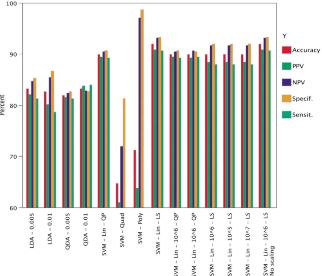
Fig. 4. Automated computer classification results for the three experiments using 14 different combinations of classifiers. The full list and parameters can be found in Table II. Results are given in terms of accuracy (proportion of all subjects correctly classified as being probable AD versus NC), sensitivity (proportion of individuals with a true positive result for probable AD), specificity (proportion of individuals with a true negative result for NC), PPV (true positive over all positive results), and NPV (true negative over all negative results). Using an SVM with linear kernel and least-square optimization (without constraint on boundary) gives the highest classification accuracy (92%, column 8). Gold standard for comparison is comprehensive clinical assessment.
3) NC versus probable AD classification using SVM.
Experi-ment 3 (SVM) was designed to assess the accuracy of
indi-vidual classification using linear and quadratic SVM under various condition.
4) Random permutations of ground truth. In order to test the robustness of the ACC methodology, Experiment
4 (Random) was designed so that random ground truth
(probable AD, NC) was assigned to each of the 150 individual study subjects; the system then attempted to classify using this information. We expected that the system would be, at best, equal to chance in classifying group membership. To test this condition, we performed 1000 trials using the best classifier as selected following the previous LDA, QDA, and SVM experiments. Only mean accuracy will be reported.
III. EXPERIMENTS ANDRESULTS
A. Study Group Demographics
There were no statistically significant differences for age be-tween the 75 probable AD (mean years;
years) and 75 NC individuals (mean years; years) (Student’s -test, ) (see Fig. 3).
B. Allowable Grey-Level and Determinant Domains
We set the variance ratio [see (5)] to 0.997, resulting in a PCA model composed of eigenvectors spanning Do-main and eigenvectors spanning Domain . We have not performed a sensitivity analysis of the classification results for different values of .
C. NC Versus Probable AD Classification Using Linear Discriminant Analyses
The best accuracy result was or 84% reached with P-to-enter set at 0.005, retaining seven variables in the final dis-criminant function (median over 150 leave-one-out trials); de-tailed results are reported in Fig. 4.
D. NC Versus Probable AD Classification Using Quadratic Discriminant Analyses
The best accuracy result was or % reached with P-to-enter set at 0.01, retaining 12 variables in the final discrim-inant function (median over 150 leave-one-out trials); detailed results are reported in Fig. 4.
E. NC Versus Probable AD Classification Using SVM
The best accuracy result was or 92% reached with a linear SVM using least-squares optimization; bounding box constraints did not influence the results. Further results on the other classifiers are reported in Fig. 4.
F. Random Permutation of Ground Truth
The mean accuracy of the linear SVM with least-squares optimization at classifying 1000 trials with randomly allocated ground truth was 49.9% (standard deviation 5.1%; maximum 68%; minimum 36%). Other results (specificity, sensitivity, PPV, NPV) not reported.
IV. DISCUSSION
A. Clinical Considerations
This paper reports results of an automated computer clas-sification technique used in the cross-sectional assessment of probable AD versus normal controls. Cross-sectional methods are potentially useful for early diagnosis, while prospective or longitudinal techniques have limited value in this regard, unless the repeat scan is very close to the baseline, e.g., less than 2–3 months, but to date this is not routinely done.
The cross-sectional accuracy for clinical assessment of prob-able AD versus normal controls, based on neurological and neu-ropsychological assessment, but verified against histopatholog-ical gold standard, is 78% (22% error rate), as mentioned in a recent consensus report [44]. When combining neuropsycho-logical testing (Mini-Mental State Examination [45]) with vi-sual rating of atrophy in the medial temporal lobe as seen from MRI [46], Wahlund and colleagues reported 95% sensitivity to probable AD. Accuracy of cross-sectional assessment of medial temporal lobe atrophy when combined with cerebrospinal fluid proteomic markers is comparable [47], and so is a linear com-bination of manually defined volumes (hippocampus, parahip-pocampal cortex) between controls and probable AD patients (93%) [13], [14].
The proposed ACC methodology achieves a level of accuracy that is similar (92%, 8% error rate) to the previous studies, albeit in a larger cohort, based on MRI information alone, and in the presence of different TR/TE and in-plane resolutions. Further, the proposed technique is completely automated (and therefore reproducible), requires no external expertise and no expert time, and is completely objective. Since MRI is noninvasive, there are no complications related to the procedure, the only limit being contra-indications to MR scanning. Thus, such a tech-nique could easily be implemented in a clinical setting and com-plement the initial assessment. This can be compared to other techniques, such as PET [48], [49] and SPECT [50], that offer sufficient specificity and sensitivity in the diagnosis of probable
AD but are minimally invasive procedures with radiation dose limitations and therefore cannot be repeatedly performed on a single patient nor used as a screening mechanism for large pop-ulations. Other MRI-based techniques such as functional mag-netic resonance imaging (fMRI) [51], MR spectroscopy [52], MR diffusion tensor [53], and MR magnetization transfer [54] show promise for the future, but are difficult to implement in a clinical setting without a dedicated research group for technical support, data acquisition and analysis. Finally, as compared to MRI, CT images lack the detailed soft-tissue information nec-essary for detecting subtle structure changes associated with the disease, especially at an early stage, even though late-stage mea-sures show promise [55].
The paper presents a tool for classifying patients; the fact that the tool classified patients well here does not, strictly speaking, imply anything about the population of patients at large. Clas-sical statistical theory tells us that the results of statistical tests on a representative sample can be used to infer properties of the population at large up to a point; but the generalizability of clas-sifier results is unclear. Therefore whether our technique can say anything about the brain patterns that probable AD subjects have in general must be further justified by studies on larger cohorts. Neuropathological confirmation is also required to replace the clinical evaluation as a gold standard in the evolution of ACC accuracy.
Biological interpretation of the information embedded in the classification function, in terms of local volume and intensity changes, remains to be performed. The separating hyperplane contains information that should be of biological importance in the study of probable AD. The differences in local volume changes should mirror the changes noticed in other reports, such as visual assessment [46], while differences in grey-level might reflect the intensity of neuronal loss induced by the neuropatho-logical changes [56], which precede volume loss as visualized on MRI. This evaluation is beyond the scope of this manuscript.
B. Methodological Considerations
Our goal is to extract pathological grey-level and deforma-tion patterns that are specific and sensitive to the task at hand, i.e., separating probable AD from NC. The registration process relies on point homology, which is of course approximate: in re-gions where there is complete homology, the displacement field will be nearly exact, up to the accuracy of the ANIMAL pro-cedure; and in regions where it is not, the result will be noisy. This latter uncertainty will be rejected in the PCA modeling, as it is uncorrelated and noncovarying. Our results further sug-gest that the system will remain robust even in multisite acqui-sitions, where systematic differences exist due to the various hardware/software configurations, not to mention platform- or vendor-specific sequences that provide similar, but never equal, contrasts [25]. The work presented here (multiple acquisitions, single site) is a necessary step in the validation of the ACC tech-nique, whereas evaluation of the procedure using multisite data will be the subject of a future manuscript.
Over determination in the creation of the reference space is not an issue as the reference group is composed of subjects taken from the ICBM studyl; these are completely independent of the study cohort. Further, by using leave-one-out cross-validation
trials, we ensured that there was no over learning in the classifi-cation stage while maximizing the amount of information avail-able. Experiment 5 (Random permutation) was aimed at demon-strating that the resulting ACC classification is not an artefactual result of over determined classification.
In this paper, the results demonstrate that SVM are margin-ally superior to other supervised classification techniques (LDA/ QDA) for the chosen task. We opted for a single classifica-tion stage using forward, stepwise regression rather than a two-stage univariate/multivariate classification scheme [57], since the latter may result in inclusion of strongly statistically sig-nificant but nonorthogonal features in the second stage, at the expense of variables with wider variance but better discrimina-tive value when combined to other features.
There are similarities and differences between this method-ology and other classification methods [21], principally Lao et
al. [19]. Both reduce a high-dimensional input vector and
at-tempt the classification on the reduction parameters, albeit using a different technique (PCA in this work; wavelet decomposition for Lao et al. [19]); both having some ability at representing spa-tial covariances in the data. The main difference between the two techniques resides in the spatial extent and choice of features. Lao et al. [19] use mass-preserved GM, WM and CSF whole brain concentration estimate maps, which are, effectively, tri-chotomized versions of the original intensity image. These, as discussed above, may prove sensitive to different acquisition pa-rameters. Our modeling is centered on the medial temporal lobe. For intensity, our approach is more in line with that of Webb
et al. [58] and sidesteps the issue of GM/WM classification, that
may suffer from over and under determination of real GM and WM volumes and/or concentrations due to tissue classification problems. The latter GM/WM variability is demonstrated in the Appendix for different contrasts, and further discussed in the work of Brickman et al. [27]. Finally, the proposed technique explicitly models local volume changes, as opposed to its im-plicit formulation within the mass-preserving framework of the RAVENS maps [59].
It is proposed to use statistical criteria (Akaike, Bayes) at a later date to determine the optimum number of eigenvectors to be retained in the separating hyperplane. Multisequence in-formation (e.g., T2) and/or multimodality (e.g., PET) may also benefit the model.
V. CONCLUSION
An immediate goal of image processing is to augment the physicians’ confidence in their diagnosis by offering quanti-tative assessments of brain images, especially in the context of pathologies such as neurodegenerative disorders. We have presented a methodology for computer-aided diagnosis and demonstrated using simulated and real data, that it appears robust to small variations in MRI acquisition parameters, as they present themselves in routine clinical use. Major strengths of this study include the number of subjects in each cohort, and the use of an ACC method that is completely automated (and, therefore, reproducible), requires no external expertise, and is completely objective. The ability of cross-sectional MRI at detecting probable AD with high accuracy is supported by the results: MR-based assessment could cut the diagnosis error
TABLE III PHANTOMSETTINGS
by a factor of two. This could have profound implication in the management of suspected AD candidates.
VI. ROLE OF THEFUNDINGSOURCES
The funding sources had no involvement in study design, col-lection, analysis, and interpretation of the data, writing of the report and in the decision to submit the paper for publication.
APPENDIX
A. Phantom Image Processing
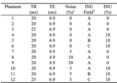
In order to assess the sensitivity of various image features to changes in TR, TE, noise, and INU, sets of coregistered phantom images were produced using the MNI BrainWeb tool (see Table III) [33]. These phantoms, built using the target volume, were by definition coregistered with it. Each MRI phantom was simulated with different imaging parameters, mimicking those present in the real dataset, making it an ideal means of assessing ACC features sensitivity.
In order to assess the sensitivity of various features to changes in acquisition parameters, our strategy was to simulate different MRI phantoms [33], varying the image acquisition parameters for each simulation, mirroring the values found in the real dataset. In the first three phantoms, TR and TE were changed; in phantoms 4–6, TR/TE were identical, but noise was added to the phantom. In phantoms 7–9, TR/TE were identical, but three different INU fields were used, and finally, in phantoms 10–12, all parameters were changed (TR, TE, noise, INU). Table III summarizes the various parameters for each phantom.
Since it is only possible to change slice thickness and not in-plane resolution with the MNI BrainWeb, and since the original image from which the phantoms are built was acquired at 1 mm isotropic resolution, we chose not to assess the variability of the measurements to different thickness/in-plane resolutions.
Different measures were then computed on each of the phantom image groups. These included the mean VOI T1-weighted intensity, in the native images (“unprocessed
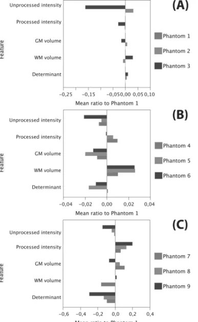
Fig. 5. Results from comparison of image features on the various Colin27 phantoms (see Table III for parameter settings). Mean value for each measure is scaled with respect to the mean value from Phantom 1. After subtraction of unity, deviations from 0 indicate sensitivity of the measurements to (A) changes in TR/TE parameters, (B) increasing levels of white additive Gaussian noise, and (C) the addition of various INU fields to the baseline phantom.
intensity”) and after the global and local affine alignment to the target (“processed intensity”) as well as the mean VOI displacement (“determinant”), after nonlinear registration and determinant computation. For example, for the intensity, labeled int:
(4)
where represents the intensity at voxel within the VOI. The total grey and white matter volumes within the VOI was also assessed, following tissue classification of the locally aligned brain [60], for example, for GM
(5)
Fig. 6. Results from comparison of image features between the baseline phantom (Phantom 1) and three phantoms combining different TR/TE values, 5% white additive Gaussian noise; and three different INU fields. The scaled mean is presented in (A) and the scaled standard deviation in (B) (no devi-ation for total GM/WM volumes). The image determinant has limited mean variations and small standard deviations when compared to other measures.
where represents if voxel has been classified as grey matter.
For each of these measures, its ratio with the base image (Phantom 1, most prevalent protocol in datasets) was calculated. Subtracting unity, any variation from 0 indicates sensitivity of the measurement to the variation in acquisition parameters. In some cases, the standard deviation ratio was also calculated in a similar fashion.
B. Experiments
Sensitivity of intensity, determinant and GM/WM volumes to changes in acquisition parameters were assessed by calculating the mean and standard deviation measures on each phantom and comparing them in turn to Phantom 1: mean variations due to TR/TE changes [Phantoms 1, 2, and 3: Fig. 5(a)]; given fixed TR/TE, mean variations due to 5%, 10%, and 20% noise [Phan-toms 4, 5 and 6; Fig. 5(b)]; given fixed TR/TE, mean variations due to three example INU fields (generated automatically by the MNI BrainWeb phantom, see [61] for details) applied with 10% weight [Phantoms 7, 8, 9; Fig. 5(c)]; finally, mean and standard deviation variations when combining all factors—three TR/TE combinations, each with a different INU field at 10% weight, and 5% noise [Phantoms 10, 11, and 12; Fig. 6(a) and (b)].
C. Results
We make the following observations after analysis of these phantoms.
• Unprocessed intensity: mean unprocessed or native in-tensity within the VOI shows variations on the order of
% to % when one changes TR/TE. For a given TR/TE combination, the impact of noise is smaller, with variations between % to %. There were varia-tions of % to % when comparing the effect of the three different INU fields. Finally, when combining the three factors, the mean unprocessed intensity within the VOI varied from % to %, whereas its standard deviation varied from 0.7% to % with respect to that of Phantom 1.
• Processed intensity: After initial processing (INU cor-rection, scaling and clamping, global and local linear alignment), the mean intensity within the VOI showed reduced variation, when compared to unprocessed results, of % to % when changing TR/TE parameters; sensitivity to noise was also reduced ( % to %), as was the effect of INU ( % to %). For all three parameters, the variation of the mean was 4.4% to 5.6%, whereas the standard deviation variation was 3.7% to 8.8%.
• Grey and white matter: volumes varied as well, indi-cating that the tissue classification process was not en-tirely immune to small contrast differences. Variations to TR/TE ranged from % to 0.6%; variations to noise from % to 2.6% and to INU from % to 10.6%. For all three parameters, variations ranged from % to %. There was no standard deviation on GM/WM vol-umes as they are single measurements for each phantom. • Determinant: variations were 0.4% to 0.9% for TR/TE
changes; % to 0.8% for noise variations and % to % for the different INU fields. Total variation for when all three parameters were combined was % to %. Standard deviation ratios for determinant were % to %, a % difference.
D. Discussion
The results of our feature sensitivity validation on phantom data showed that the selected features (unprocessed or processed intensity, GM/WM volumes, and determinants) exhibited small to large variations when different contrasts, noise, and INU were present in the images, other variables (e.g., resolution, registra-tion) remaining fixed.
GM/WM volume estimations were not immune to contrast differences. Whereas the contrast differences drive the classifi-cation process, one might have expected that the a priori spa-tial distribution knowledge embedded in the classification al-gorithm would have glossed over those differences. To be fair, this was single-modality classification (i.e., only T1-weighted images on input); it is assumed that multispectral images (e.g., with T2, PD) increase the accuracy of the classification. Finally, there was no estimation of partial volumes effects.
The mean intensity after processing (INU correction, scaling, clamping, global and local linear registration) was more robust than the unprocessed intensity. This seems to indicate that signal intensity, and possibly intensity-derived statistical or structural texture features (provided they are estimated in 3-D and are ro-tation-invariant), can act as valid features for ACC methodolo-gies in the case of varying sequence parameters and acquisition irregularities. The smoothing effect on differences of the INU
correction algorithm of Sled et al. was also highlighted in a re-cent multisite longitudinal study [25]. Determinant estimation showed sensitivity to INU fields but overall, displayed the most compact distribution, with nearly the smallest mean differences and the lowest standard deviation ratios of all measures. The use of geometrical information (e.g., Jacobian determinants) as op-posed to intensity-based information, ensures that the technique is less sensitive to image transformations, an issue that was also mentioned by Thirion [62].
ACKNOWLEDGMENT
The authors wish to acknowledge ICBM for the data and anonymous reviewers for their insights into improving the manuscript.
REFERENCES
[1] H. Braak and E. Braak, “Evolution of the neuropathology of alzheimer’s disease,” Acta Neurol. Scand. Suppl., vol. 165, pp. 3–12, 1996.
[2] J. Ashburner, J. G. Csernansky, C. Davatzikos, N. C. Fox, G. B. Frisoni, and P. M. Thompson, “Computer-assisted imaging to assess brain structure in healthy and diseased brains,” Lancet Neurol., vol. 2, pp. 79–88, 2003.
[3] O. Hansson, H. Zetterberg, P. Buchhave, E. Londos, K. Blennow, and L. Minthon, “Association between CSF biomarkers and incipient alzheimer’s disease in patients with mild cognitive impairment: A follow-up study,” Lancet Neurol., vol. 5, pp. 228–234, 2006. [4] B. Dubois, H. H. Feldman, C. Jacova, S. T. Dekosky, P.
Barberger-Gateau, J. Cummings, A. Delacourte, D. Galasko, S. Gauthier, G. Jicha, K. Meguro, J. O’Brien, F. Pasquier, P. Robert, M. Rossor, S. Salloway, Y. Stern, P. J. Visser, and P. Scheltens, “Research criteria for the di-agnosis of Alzheimer’s disease: Revising the nincds-adrda criteria,”
Lancet Neurol., vol. 6, pp. 734–46, 2007.
[5] P. A. Freeborough and N. C. Fox, “MR image texture analysis applied to the diagnosis and tracking of Alzheimer’s disease,” IEEE Trans.
Med. Imag., vol. 17, no. 3, pp. 475–479, Jun. 1998.
[6] G. B. Frisoni, C. Testa, A. Zorzan, F. Sabattoli, A. Beltramello, H. Soininen, and M. P. Laakso, “Detection of grey matter loss in mild alzheimer’s disease with voxel based morphometry,” J. Neurol.
Neuro-surg. Psychiatry, vol. 73, pp. 657–664, 2002.
[7] P. M. Thompson, K. M. Hayashi, G. I. De Zubicaray, A. L. Janke, S. E. Rose, J. Semple, M. S. Hong, D. H. Herman, D. Gravano, D. M. Doddrell, and A. W. Toga, “Mapping hippocampal and ventricular change in alzheimer disease,” NeuroImage, vol. 22, pp. 1754–1766, 2004.
[8] G. B. Frisoni, F. Sabattoli, A. D. Lee, R. A. Dutton, A. W. Toga, and P. M. Thompson, “In vivo neuropathology of the hippocampal formation in AD: A radial mapping MR-based study,” in NeuroImage, 2006. [9] J. G. Csernansky, L. Wang, S. Joshi, J. P. Miller, M. Gado, D. Kido, D.
McKeel, J. C. Morris, and M. I. Miller, “Early DAT is distinguished from aging by high-dimensional mapping of the hippocampus. de-mentia of the alzheimer type,” Neurology, vol. 55, pp. 1636–1643, 2000.
[10] P. M. Thompson, K. M. Hayashi, G. de Zubicaray, A. L. Janke, S. E. Rose, J. Semple, D. Herman, M. S. Hong, S. S. Dittmer, D. M. Dod-drell, and A. W. Toga, “Dynamics of gray matter loss in Alzheimer’s disease,” J. Neurosci., vol. 23, pp. 994–1005, 2003.
[11] D. Chan, J. C. Janssen, J. L. Whitwell, H. C. Watt, R. Jenkins, C. Frost, M. N. Rossor, and N. C. Fox, “Change in rates of cerebral atrophy over time in early-onset alzheimer’s disease: Longitudinal MRI study,”
Lancet., vol. 362, pp. 1121–1122, 2003.
[12] J. P. Lerch, J. C. Pruessner, A. Zijdenbos, H. Hampel, S. J. Teipel, and A. C. Evans, “Focal decline of cortical thickness in alzheimer’s disease identified by computational neuroanatomy,” Cereb Cortex, vol. 15, pp. 995–1001, 2005.
[13] C. Pennanen, M. Kivipelto, S. Tuomainen, P. Hartikainen, T. Han-ninen, M. P. Laakso, M. Hallikainen, M. Vanhanen, A. Nissinen, E. L. Helkala, P. Vainio, R. Vanninen, K. Partanen, and H. Soininen, “Hip-pocampus and entorhinal cortex in mild cognitive impairment and early AD,” Neurobiol. Aging, vol. 25, pp. 303–310, 2004.
[14] S. J. Teipel, J. C. Pruessner, F. Faltraco, C. Born, M. Rocha-Unold, A. Evans, H. J. Moller, and H. Hampel, “Comprehensive dissection of the medial temporal lobe in AD: measurement of hippocampus, amyg-dala, entorhinal, perirhinal and parahippocampal cortices using MRI,”
J. Neurol., vol. 253, pp. 794–800, 2006.
[15] J. C. Pruessner, L. M. Li, W. Serles, M. Pruessner, D. L. Collins, N. Kabani, S. Lupien, and A. C. Evans, “Volumetry of hippocampus and amygdala with high-resolution mri and three-dimensional analysis software: Minimizing the discrepancies between laboratories,”
Cere-bral Cortex, vol. 10, pp. 433–442, 2000.
[16] J. C. Pruessner, S. Kohler, J. Crane, M. Pruessner, C. Lord, A. Byrne, N. Kabani, D. L. Collins, and A. C. Evans, “Volumetry of temporopolar, perirhinal, entorhinal and parahippocampal cortex from high-resolu-tion MR images: Considering the variability of the collateral sulcus,”
Cerebral Cortex, vol. 12, pp. 1342–1353, 2002.
[17] S. Duchesne, N. Bernasconi, A. Bernasconi, and D. L. Collins, “MR-based neurological disease classification methodology: Application to lateralization of seizure focus in temporal lobe epilepsy,” NeuroImage, vol. 29, pp. 557–566, 2006.
[18] Y. Liu, L. Teverovskiy, O. Carmichael, R. Kikinis, M. Shenton, C. S. Carter, V. A. Stenger, S. Davis, H. Aizenstein, J. T. Becker, O. L. Lopez, and C. C. Meltzer, “Discriminative MR image feature analysis for automatic schizophrenia and alzheimer aäôs disease classification,” presented at the Med. Image Comput. Comput. Assist. Intervention Conf., Saint-Malo, France, 2004.
[19] Z. Lao, D. Shen, Z. Xue, B. Karacali, S. M. Resnick, and C. Da-vatzikos, “Morphological classification of brains via high-dimensional shape transformations and machine learning methods,” NeuroImage, vol. 21, pp. 46–57, 2004.
[20] L. G. Apostolova, R. A. Dutton, I. D. Dinov, K. M. Hayashi, A. W. Toga, J. L. Cummings, and P. M. Thompson, “Conversion of mild cog-nitive impairment to alzheimer disease predicted by hippocampal at-rophy maps,” Arch. Neurol., vol. 63, pp. 693–699, 2006.
[21] P. Golland, W. E. Grimson, M. E. Shenton, and R. Kikinis, “Detection and analysis of statistical differences in anatomical shape,” Med. Image
Anal., vol. 9, pp. 69–86, 2005.
[22] J. M. Fitzpatrick and M. Sonka, “Handbook of medical imaging, volume 2. medical image processing and analysis,” in Int. Soc. Optical
Eng., 2000.
[23] P. Tofts, Quantitative MRI of the Brain: Measuring Changes Caused
by Disease. New York: Wiley, 2003.
[24] G. M. Preboske, J. L. Gunter, C. P. Ward, and C. R. Jack Jr., “Common MRI acquisition non-idealities significantly impact the output of the boundary shift integral method of measuring brain atrophy on serial MRI,” NeuroImage, vol. 30, pp. 1196–1202, 2006.
[25] A. D. Leow, A. D. Klunder, C. R. Jack Jr., A. W. Toga, A. M. Dale, M. A. Bernstein, P. J. Britson, J. L. Gunter, C. P. Ward, J. L. Whitwell, B. J. Borowski, A. S. Fleisher, N. C. Fox, D. Harvey, J. Kornak, N. Schuff, C. Studholme, G. E. Alexander, M. W. Weiner, and P. M. Thompson, “Longitudinal stability of MRI for mapping brain change using tensor-based morphometry,” NeuroImage, vol. 31, pp. 627–640, 2006. [26] S. Duchesne and K. De Sousa, “Predicting MCI progression to AD via
automated analysis of T1 weighted MR image intensity,” Alzheimer’s
Dementia, vol. 83, 2005.
[27] A. M. Brickman, C. Habeck, E. Zarahn, J. Flynn, and Y. Stern, “Struc-tural MRI covariance patterns associated with normal aging and neu-ropsychological functioning,” Neurobiol. Aging, vol. 28, pp. 284–295, 2007.
[28] Y. Fan and N. Batmanghelich et al., “Spatial patterns on brain atrophy in MCI patients, identified via high-dimensional pattern classification. predict subsequent cognitive decline,” NeuroImage, vol. 39, no. 4, pp. 1731–1743, 2008.
[29] A. Shiino, T. Watanabe, K. Maeda, E. Kotani, I. Akiguchi, and M. Msuda, “Four subgroups of Alzheimer’s disease based on patterns of at-rophy using VBM and a unique pattern for early onset disease,”
Neu-roImage, vol. 33, pp. 17–26, 2006.
[30] S. Duchesne, J. Pruessner, S. Teipel, H. Hampel, and D. L. Collins, “Successful AD and MCI differentiation from normal aging via au-tomated analysis of MR image features,” Alzheimer’s Dementia: J.
Alzheimer’s Assoc., vol. 1, p. 43, 2005.
[31] J. C. Mazziotta, A. W. Toga, A. Evans, P. Fox, and J. Lancaster, “A probabilistic atlas of the human brain: Theory and rationale for its de-velopment. the international consortium for brain mapping (ICBM),”
NeuroImage, vol. 2, pp. 89–101, 1995.
[32] G. McKhann, D. Drachman, M. Folstein, R. Katzman, D. Price, and E. M. Stadlan, “Clinical diagnosis of Alzheimer’s disease: Report of the NINCDS-ADRDA work group under the auspices of department of health and human services task force on alzheimer’s disease,”
Neu-rology, vol. 34, pp. 939–944, 1984.
[33] D. L. Collins, A. P. Zijdenbos, V. Kollokian, J. G. Sled, N. J. Kabani, C. J. Holmes, and A. C. Evans, “Design and construction of a realistic digital brain phantom,” IEEE Trans. Med. Imag., vol. 17, pp. 463–468, 1998.
[34] J. G. Sled, A. P. Zijdenbos, and A. C. Evans, “A nonparametric method for automatic correction of intensity nonuniformity in MRI data,” IEEE
Trans. Med. Imag., vol. 17, no. 1, pp. 87–97, Feb. 1998.
[35] D. L. Collins and A. C. Evans, “ANIMAL: Validation and applications of non-linear registration based segmentation,” Int. J. Pattern Recognit.
Artif. Intell., vol. 11, pp. 1271–1294, 1997.
[36] A. Collignon, F. Maes, D. Delaere, D. Vandermeulen, P. Suetens, and G. Marchal, “Automated multi-modality image registration based on information theory,” in Information Processing in Medical Imaging. Norwell, MA: Kluwer, 1995.
[37] F. Maes, A. Collignon, D. Vandermeulen, G. Marchal, and P. Suetens, “Multimodality image registration by maximization of mutual infor-mation,” IEEE Trans. Med. Imag., vol. 16, no. 2, pp. 187–198, Apr. 1997.
[38] M. K. Chung, K. J. Worsley, T. Paus, C. Cherif, D. L. Collins, J. N. Giedd, J. L. Rapoport, and A. C. Evans, “A unified statistical approach to deformation-based morphometry,” NeuroImage, vol. 14, pp. 595–606, 2001.
[39] T. F. Cootes, G. J. Edwards, and C. J. Taylor, “Active appearance models,” IEEE Trans. Pattern Anal. Mach. Intell., vol. 23, no. 6, pp. 681–685, Jun. 2001.
[40] S. Duchesne, J. Pruessner, and D. L. Collins, “Appearance-based seg-mentation of medial temporal lobe structures,” NeuroImage, vol. 17, pp. 515–531, 2002.
[41] R. O. Duda, P. E. Hart, and D. G. Stork, “Pattern classification,” in
Wiley-Interscience, 2001.
[42] C. J. Burges, “A tutorial on support vector machines for pattern recog-nition,” Data Mining Knowledge Discovery, vol. 2, pp. 121–167, 1998. [43] G. C. Cawley and N. L. Talbot, “Fast exact leave-one-out cross-vali-dation of sparse least-squares support vector machines,” Neural Netw., vol. 17, pp. 1467–1475, 2004.
[44] M. Weiner, M. Albert, C. DeCarli, S. de Kosky, M. de Leon, N. L. Foster, N. Fox, R. Frank, R. Frackowiak, C. Jack, W. Jagust, D. Knopman, J. Morris, R. C. Petersen, E. Reiman, P. Scheltens, G. Small, H. Soininen, L. Thal, L. Wahlund, W. Thies, and K. Khacha-turian, The use of MRI and PET for clinical diagnosis of dementia and investigation of cognitive impairment: A consensus report Alzheimer’s Assoc., 2005.
[45] M. F. Folstein, S. E. Folstein, and P. R. McHugh, ““Mini-mental state” A practical method for grading the cognitive state of patients for the clinician,” J. Psychiatr. Res., vol. 12, pp. 189–198, 1975.
[46] L. O. Wahlund, P. Julin, S. E. Johansson, and P. Scheltens, “Visual rating and volumetry of the medial temporal lobe on magnetic reso-nance imaging in dementia: A comparative study,” J. Neurol.
Neuro-surg. Psychiatry, vol. 69, pp. 630–635, 2000.
[47] N. S. Schoonenboom, W. M. van der Flier, M. A. Blankenstein, F. H. Bouwman, G. J. Van Kamp, F. Barkhof, and P. Scheltens, “CSF and MRI markers independently contribute to the diagnosis of alzheimer’s disease,” Neurobiol. Aging, 2007.
[48] W. E. Klunk, H. Engler, A. Nordberg, Y. Wang, G. Blomqvist, D. P. Holt, M. Bergstrom, I. Savitcheva, G. F. Huang, S. Estrada, B. Ausen, M. L. Debnath, J. Barletta, J. C. Price, J. Sandell, B. J. Lopresti, A. Wall, P. Koivisto, G. Antoni, C. A. Mathis, and B. Langstrom, “Imaging brain amyloid in alzheimer’s disease with Pittsburgh com-pound-B,” Ann. Neurol., vol. 55, pp. 306–319, 2004.
[49] A. Nordberg, “PET imaging of amyloid in Alzheimer’s disease,”
Lancet Neurol., vol. 3, p. 519, 2004.
[50] F. J. Bonte, M. F. Weiner, E. H. Bigio, and C. L. White, 3rd, “SPECT imaging in dementias,” J. Nucl. Med., vol. 42, pp. 1131–1133, 2001. [51] S. C. Johnson, A. J. Saykin, L. C. Baxter, L. A. Flashman, R. B.
San-tulli, T. W. McAllister, and A. C. Mamourian, “The relationship be-tween fMRI activation and cerebral atrophy: Comparison of normal aging and alzheimer disease,” NeuroImage, vol. 11, pp. 179–187, 2000. [52] K. Kantarci, C. R. Jack Jr., Y. C. Xu, N. G. Campeau, P. C. O’Brien, G. E. Smith, R. J. Ivnik, B. F. Boeve, E. Kokmen, E. G. Tangalos, and R. C. Petersen, “Regional metabolic patterns in mild cognitive impairment and alzheimer’s disease: A 1H MRS study,” Neurology, vol. 55, pp. 210–217, 2000.
[53] R. Stahl, O. Dietrich, S. Teipel, H. Hampel, M. F. Reiser, and S. O. Schoenberg, “Assessment of axonal degeneration on Alzheimer’s disease with diffusion tensor MRI,” Radiologe, vol. 43, pp. 566–575, 2003.
[54] N. J. Kabani, J. G. Sled, and H. Chertkow, “Magnetization transfer ratio in mild cognitive impairment and dementia of Alzheimer’s type,”
NeuroImage, vol. 15, pp. 604–610, 2002.
[55] G. B. Frisoni, R. Rossi, and A. Beltramello, “The radial width of the temporal horn in mild cognitive impairment,” J. Neuroimag., vol. 12, pp. 351–354, 2002.
[56] L. O. Wahlund and K. Blennow, “Cerebrospinal fluid biomarkers for disease stage and intensity in cognitively impaired patients,” Neurosci.
Lett., vol. 339, pp. 99–102, 2003.
[57] E. Duchesnay, A. Cachia, A. Roche, D. Riviere, Y. Cointepas, D. Papadopoulos-Orfanos, M. Zilbovicius, J. L. Martinot, J. Regis, and J.-F. Mangin, “Classification based on cortical folding patterns,” IEEE
Trans. Med. Imag., vol. 26, no. 4, pp. 553–565, Apr. 2007.
[58] J. Webb, A. Guimond, P. Eldridge, D. Chadwick, J. Meunier, J. P. Thirion, and N. Roberts, “Automatic detection of hippocampal atrophy on magnetic resonance images,” Magn. Reson. Imag., vol. 17, pp. 1149–1161, 1999.
[59] C. Davatzikos, A. Genc, D. Xu, and S. M. Resnick, “Voxel-based morphometry using the RAVENS maps: Methods and validation using simulated longitudinal atrophy,” NeuroImage, vol. 14, pp. 1361–1369, 2001.
[60] C. A. Cocosco, A. P. Zijdenbos, and A. C. Evans, “A fully automatic and robust brain MRI tissue classification method,” Med. Image Anal., vol. 7, pp. 513–527, 2003.
[61] R. K. Kwan, A. C. Evans, and G. B. Pike, “MRI simulation-based eval-uation of image-processing and classification methods,” IEEE Trans.
Med. Imag., vol. 18, no. 11, pp. 1085–1097, Nov. 1999.
[62] J. P. Thirion and G. Calmon, “Deformation analysis to detect and quan-tify active lesions in three-dimensional medical image sequences,”