Improved crack tip enrichment functions and integration for crack modeling using the extended finite element method

HAL Id: hal-01006957

https://hal.archives-ouvertes.fr/hal-01006957

Submitted on 20 Feb 2018

HAL is a multi-disciplinary open access

archive for the deposit and dissemination of

sci-entific research documents, whether they are

pub-lished or not. The documents may come from

teaching and research institutions in France or

abroad, or from public or private research centers.

L’archive ouverte pluridisciplinaire HAL, est

destinée au dépôt et à la diffusion de documents

scientifiques de niveau recherche, publiés ou non,

émanant des établissements d’enseignement et de

recherche français ou étrangers, des laboratoires

publics ou privés.

Improved crack tip enrichment functions and integration

for crack modeling using the extended finite element

method

Nicolas Chevaugeon, Nicolas Moës, Hans Minnebo

To cite this version:

Nicolas Chevaugeon, Nicolas Moës, Hans Minnebo. Improved crack tip enrichment functions and

integration for crack modeling using the extended finite element method. International Journal for

Multiscale Computational Engineering, Begell House, 2013, 11 (6), pp.597-631.

�10.1615/IntJMult-CompEng.2013006523�. �hal-01006957�

IMPROVED

CRACK TIP ENRICHMENT FUNCTIONS AND

INTEGRATION

FOR CRACK MODELING USING THE

EXTENDED

FINITE ELEMENT METHOD

Nicolas Chevaugeon, Nicolas Moës & Hans Minnebo

LUNAM Universite, GeM UMR6183, Ecole Centrale de Nantes, 1 Rue de la Noe, 44321, Nantes, France

∗_Address

all correspondence to Nicolas Chevaugeon, E-mail: nicolas.chevaugeon@ec-nantes.fr

This paper focuses on two improvements of the extended finite element method (X-FEM) in the context of linear fracture mechanics. Both improve the accuracy and the robustness of the X-FEM. In a first contribution, a new enrichment strategy is proposed to take into account the singular stress field at the crack tip that is meant to replace the traditional four-crack-tip enrichment functions. The efficiency of the new approach is demonstrated on mesh convergence experi-ments for two-dimensional straight and curved crack problems, using first- and second-order shape functions, both in terms of convergence rates and in terms of condition number of the system to solve. The second contribution revisits the problem of the numerical integration of the stiffness operator when singular functions like the tip enrichment functions are used. An original algorithm to build accurate and fast integration rules for elements in the enrichment zone, touch-ing the crack tip singularity, or not, is presented. The effects on convergence rate of the choice of the integration rule are illustrated on numerical examples.

KEY WORDS: X-FEM, cracks, singular function integration, LEFM 1. INTRODUCTION

The paper presents some improvements to the extended finite element method (X-FEM) in the context of linear fracture mechanics. The goal is to provide better convergence rate and robustness to the method. Most FEM industrial codes provide up to a second-order finite element, with a corresponding optimal second-order h convergence rate of the energy norm error when applied to regular problems. The X-FEM, beyond relaxing the constraint on the mesh, also has the potential to reach optimal convergence rate in the presence of a stress singularity such as a crack. It is generally considered achieved when first-order shape functions are used (B´echet et al., 2005; Laborde et al., 2005). Using a geometrical enrichment strategy and a sufficiently accurate integration rule, a first-order convergence rate has already been demonstrated. Moving to higher order while keeping the optimal convergence rate is much more difficult. This is our ultimate goal and the contributions of this paper are steps toward that goal.

The outline of the paper is as follows: In the first section, the X-FEM modeling strategy for cracks is briefly recalled, with references and comparisons to the variants introduced by the generalized finite element method (G-FEM). Special care is focused toward the definition of the enrichment zone, either topological or geometrical. In this first section, the vectorial crack tip enrichment strategy is be presented, along with some details on its implementation. The second section is devoted to the analysis and the construction of a new quadrature rule meant to reduce the integration error in the stiffness matrix, due to the presence of singular terms coming from the tip enrichment functions. In the last section, the proposed improvements are tested on some benchmarks where high-order accuracy is achieved. Optimal order of convergence is obtained, for both first- and second-order shape functions, with a reasonable condition number for the stiffness matrix, compared to the previous method. Lastly, taking advantage of the structure of the vector enrichment functions, a very fast stress intensity factor extractor is presented. Its usefulness as compared to G-theta domain integral methods is discussed. Finally, the paper ends with some conclusions.

2. THE X-FEM MODELING OF CRACKS 2.1 Problem Statement

We place ourselves within the context of linear elasticity. On a discretized domain Ωh, where h is a discretization parameter (element size) bounded by Γh, the weak form of the discretized equilibrium equations may be written as follows:

Find uh, the discretized displacement field ∈ Vh, such that

Z Ωh B(uh, vh)dΩ = Z Γt L(vh)dΓ∀vh∈ Vh0 (1.1)

where Vhis the trial space for the displacement field, over the mesh that discretizes the domain Ω, that fulfills the Dirichlet boundary condition on Γh_u, and Vh₀ is the corresponding space with a homogeneous Dirichlet boundary condition. B is a bilinear operator, defined as B(u, v) = ∇suh_{: D : ∇}s_vh_{, where ∇}S_{u is the symmetric part of the}

gradient tensor of u (e.g., the linearized strain tensor), and D is the fourth-order elasticity tensor. L is a linear operator corresponding to the Neumann boundary condition on Γt : L(u) = t.u, where t represents the prescribed tractions

known on Γt.

The domain Ω is then cut by a traction-free crack. In the context of X-FEM, the mesh does not conform to the crack and alternative representations for the geometry of the crack need to be used.

2.2 Geometric representation of the crack

The modeling of three-dimensional (3D) cracks not aligned with the mesh using the partition of unity was first devel-oped in Sukumar et al. (2000). The description of the crack location was explicit in this paper.

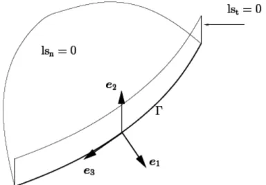
Later, in Mo¨es et al. (2002), a more flexible level set representation was introduced, the representation used in the present work, which we describe in the following. The crack location is given by two level sets. The normal level set, lsn, corresponds to the signed distance to the crack surface. The tangential level set lstcorresponds the signed distance to the front (or to be more precise, the distance to a surface passing through the front and orthogonal to the crack surface). The crack front is given by the set of points were both lsnand lstare zero, whereas the crack is given by the set of points for which lsn= 0 and lst≤ 0. The iso-zero of the two level sets are depicted in Fig. 1 close to a crack front portion.

Numerically, the level sets are discretized as a linear finite element approximation, over the mesh that is used for the computation of the displacement field. It is, of course, possible to use another mesh to represent the level set. For example, it was proposed to represent the level set on a finer mesh, or on a structured or octree type of mesh (Legrain et al., 2012; Prabel et al., 2007; Sukumar et al., 2008). The latter versions are sometimes more memory efficient, and more efficient propagation algorithms can be used to update the position of the crack when performing crack propagation analysis. Using an implicit representation of the crack such as the one presented, has some drawbacks. Indeed, the crack surface, if simple enough, could be described by a parametric surface, or by a mesh. The memory cost of such a representation would be in most cases much smaller than the cost of representing two discrete level sets over a whole mesh. Those claims could nonetheless be more balanced, since the level sets need only to be defined in a narrow band containing the crack surface (Osher and Fedkiw, 2002; Sethian, 1999).

In the context of crack propagation, the crack front represented by the level set lstis able to take any topology. Updating a mesh of the crack front, on the other hand, can be more difficult.

2.3 Crack Tip Enrichment: Classical Version

The commonly used X-FEM approximation field is as follows. If no crack is present, the displacement field u(x) over the body located in Ω is approximated by

uh(x) = X

i∈[1:dim]

X

I∈N

NI(x)uIiEi (1.2)

where N is the set of all nodes in the mesh, NI are the classical C0shape functions, and uIiare the displacement

degrees of freedom attached to node I in direction Ei, where the Ei form a global orthonormal basis, and dim is

the number of spacial dimensions of the problem. Introducing a crack in the mesh yields the following enriched approximation: uh(x) = X i∈[1:dim] X I∈N NI(x)uIiEi+ X i∈[1:dim] X I∈Ncrack NI(x)H[lsn(x)]hIiEi + X i∈[1:dim] X I∈Ntip X α NI(x)Fα[lsn(x), lst(x)]aIiαEi (1.3) in which

– Ncrackis the set of nodes whose support (union of the elements connected to the node) is completely cut into two by the crack. These nodes are enriched by the generalized Heaviside function:

H[lsn(x)] = sign[lsn(x)] (1.4)

sign(x) = −1 if x < 0, sign(x) = +1 if x ≥ = 0.

– Ntipis the set of nodes enriched by the tip enrichment functions:

[Fα] = · √ r sinθ 2, √ r cosθ 2, √ r sinθ 2sin θ, √ r cosθ 2sin θ ¸ (1.5) where r = q lsn2+ lst2, θ = tan−1 µ lsn lst ¶ (1.6)

– hIiare the degrees of freedom associated to the Heaviside enrichment function attached to node I, in direction i.

– aIiαare the degrees of freedom associated to the α crack tip enrichment function attached to node I, in

The set Ntipmust at least contain the nodes whose supports touch the crack front. Similarly to what was introduced in B´echet et al. (2005) and Laborde et al. (2005), we can distinguish topological and geometrical enrichment. We denote by Vgeo(R) the set of elements for which at least one node is at a distance r to the crack front smaller or

equal to R. The distance r is computed by Eq. (1.6). We denote by Vtopo(n) the set of elements composing n layers

of elements around the front. The precise definition of the layers follows. The first layer contains all the elements touching the front. The second layer is defined as the elements connected to the nodes of the elements of the first layer. The third layer is defined as the elements connected to the nodes of the elements of the second layer and so on. For all the numerical examples presented in the presented here, we use the geometrical enrichment strategy where

Ntipis the set of nodes of Vgeo(R). It was shown, for example, in B´echet et al. (2005) that it was required to obtain an optimal rate of convergence in energy error norm. For the rest of the paper, we refer to the use of the four Fαcrack tip enrichment functions as the scalar enrichment or scalar tip enrichment to differentiate with the new enrichment that is presented in the next section.

2.4 Crack Tip Enrichment: Updated Version 2.4.1 Presentation

In the present paper we propose to investigate an updated version of the X-FEM enrichment we just discussed. The main difference is that instead of using the four Fαscalar enrichment functions, we propose to use three Kα vector enrichment functions. Equation (1.3) then reads

u(x) = X i∈[1:dim] X I∈N NI(x)uIiEi+ X i∈[1:dim] X I∈Ncrack NI(x)H[lsn(x)]hIiEi + X I∈Ntip X α NI(x)Kα[lsn(x), lst(x)]aIα (1.7)

In this updated version, only the last sum differs slightly. The aIαare now scalar degrees of freedom and the vectorial

nature of the displacement field is embedded in the enrichment functions. We make the choice to use three vector enrichment functions that are a dimensionless version of the three Irwin asymptotic opening modes (Irwin, 1957).

K1= √ r cosθ 2(κ − cos θ)[e1(x) + e2(x)] (1.8) K2= √ r sinθ 2(κ + 2 + cos θ)e1(x) + √ r cosθ 2(κ − 2 cos θ)e2(x) (1.9) K3= √ r sinθ 2e3(x) (1.10)

where κ = 3–4ν, with ν the Poisson ratio, in 3D or the plane strain case.

2.4.2 Bibliographic Discussion

While the idea of using these enrichment functions seemed original to us at the time of development, further review of the bibliography showed that the idea was already used in a similar form in the G-FEM context. While G-FEM and X-FEM methods appeared approximately at the same time and were both applications of the partition-of-unity method and were both applied to the modelization of cracks, they were initially quite different. The two methods evolved since then borrowing ideas from each other to the point that it is difficult to distinguish them now (Belytschko and Fries, 2010). If we refer to early applications for cracks (1999, 2000) the introduction of discontinuity inside an element was done using a discontinuous partition of unity in the G-FEM, while in the case of the X-FEM, the discontinuity was introduced via Heaviside enrichment multiplied by a linear, continuous partition of unity. In the original G-FEM, the displacement space is defined as

where the φi(x) are constructed from Shepard function, using the visibility criteria, and the Niare the classical finite

element shape functions. In the original X-FEM the displacement space is defined as

u =XqiNi+

X

hiNiH[lsn(x)] (1.12) where the Niare the classical finite element shape functions and H is the Heaviside function, defined on top of the

normal level set that gives the distance to the crack surface. More recent papers in G-FEM seem to have adopted a formulation closer to X-FEM, where the discontinuity is now introduced via the enrichment. Enriching the elements touching the crack tip directly with vectorial functions that are the asymptotic expansion of the exact solution ap-peared, to our knowledge, in G-FEM in Duarte et al. (2000), where it was applied to describe corners or wedges and, at the limit when the angle goes to 0, cracks. The discrete displacement field is enriched around a corner using vecto-rial functions that are directly the asymptotic expansion of the exact solution. In this paper, the mesh was conformed to the corner. In the following paper (Duarte et al., 2001), the method is explicitly applied to cracks and the “WA” criteria is used to choose a node enriched by the asymptotic expansion. WA criteria refer to “wrap around nodes,” e.g., all nodes belonging to elements that intersect the crack front. At this time, the enrichment is therefore only “topo-logic” in our designation. The enrichment proposed in this paper is indeed the same as the one proposed in Duarte et al. (2000), but at the time of this paper, the need to have a geometric criteria instead of a topological in order to get optimal convergence order was not yet realized, and the idea of using a level set to represent the crack was not used. In a more recent paper (Pereira et al., 2009), the same group proposed another enrichment strategy, inspired by the initial one, where the three vectorial asymptotic displacement field functions are split in six enrichment functions according to the tangential and normal directions. This approach permits the precise description of the direction of the crack to be avoided, while still limiting the number of degrees of freedom per enriched node to 6 (to be compared to the 12 enrichment functions with scalar enrichment). In this paper, the author used topologic enrichment, claiming that geometrical enrichment only works for planar crack. As shown in the examples Section 3, the geometric enrichment works perfectly in our case, even for nonplanar cracks. Until now, all papers that model crack using the X-FEM and crack tip enrichment used the basis proposed initially, i.e., the four scalar enrichment functions 1.5, applied separately in each space direction. In view of the bibliography, the originality of the present paper is therefore not to use the presented vector enrichment functions, but rather to use them in the context of geometrical enrichment, based upon a level set representation of the crack and realizing the consequences on the conditioning of the stiffness matrix, while showing an optimal rate of convergence for both straight and curved cracks.

2.4.3 Implementation Issues

The three vector enrichment functions (1.8–1.10) are defined as a function of the local crack basis, that, in general depends on x. Therefore, to ensure continuity of the displacement field, at first sight, it seems that the local basis has to be defined continuously over the enrichment zone. It would mean that one needs to build from the gradient of the discretized level set, a continuous field of moving local basis. Furthermore, when computing the gradient of the proposed enriched function, a curvature term (∂ei)/xjwould appear. Even if this term might be neglected when

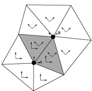
the curvature of the crack is small compared to the element size in the enrichment zone, it seems a difficult task to implement a robust version using this point of view. In fact, we propose a much easier alternative. We propose to define a local crack basis discretization per enriched node. This local basis needs only to be defined over the support of the enriched node. Since the enrichment function associated to an enriched node is multiplied by the finite element shape functions associated to the node, the resulting function is always zero on the boundary and outside of the support. This alleviates the continuity constrain over the local crack basis discretization: for each enriched node, its associated local crack basis discretization needs only to be continuous over its support, resulting in an overall continuous field. To simplify the discretization even more, we choose a constant approximation of each local crack basis per enriched node over the node’s support. This permits the computation of the curvature term to be avoided. Figure 2 illustrates a typical situation. On this small mesh, suppose that only nodes A and B are enriched. When computing the stiffness matrix on the gray element, the contribution of the enrichment of node A and B must be taken into account. When computing the enrichment attached to node A, we use the local basis defined for the support of node A, and respectively, when

FIG. 2: The support of two nodes (large dot), with two local basis, one belonging to each node.

computing the enrichment attached to node B, we use the local basis defined for the support of node B. The number of local basis defined over an element is equal to the number of supports of enriched nodes this element is a part of. The enrichment function is now a function of the enriched node. This is reflected in the following rewriting of the last term of Eq. (1.7): X I∈Ntip X α NI(x)KIα[lsn(x), lst(x)]aIα (1.13)

where the dependence of the enrichment function on the node it is attached to appears clearly, and where

KI 1= √ r cosθ 2(κ − cos θ)(e I 1+ eI2) (1.14) KI 2= √ r sinθ 2(κ + 2 + cos θ)e I 1+ √ r cosθ 2(κ − 2 cos θ)e I 2 (1.15) KI 3= √ r sinθ 2e I 3 (1.16)

where eI_i is the discretized value of the ith basis vector of the moving local axis, at node I. In our implementation of the X-FEM, the two level sets are discretized with linear shape function over the mesh. We can therefore compute their gradient, constant in each element, and from them construct a constant orthogonal basis per element that approximates the local crack tip axis. But we need a constant value per support. To obtain this value, we simply take the weighted average of the constant gradients over each element in the support of the enriched node, and from these values, construct an orthogonal basis. This scheme is very efficient and easy to implement.

This concludes our first part. We reviewed the X-FEM for linear fracture mechanics, covering the representation of the geometry and proposing a different crack tip enrichment strategy. Our vector enrichment strategy is tested and discussed more in part 3, but first we must cover the problem of the integration of the elasticity operator (the stiffness matrix) over enriched elements.

3. INTEGRATION RULE

Integration of the bilinear form B(vh, uh), for each enriched element, is known to be problematic. Indeed, leading terms of the expression to integrate include terms such as 1/r due to the tip enrichment, and the functions to integrate

are discontinuous across the crack surface. In the context of two- or three-dimensional problems, there is no hope for an exact integration of the bilinear form over a tip-enriched element. Numerical integration is, of course, needed. From the start of the X-FEM, some papers already tried to deal with this issue: how to obtain an efficient integration scheme so that the error in the integration of the bilinear form doesn’t pollute the results so much as it degrades the convergence properties. Recent references on the subject are, among others, B´echet et al. (2005), Park et al. (2009), and Mousavi and Sukuvar (2010), which used ideas developed outside of the X-FEM context in Duffy (1982) and Nagarajan and Mukherjee (1993). The first step was to cut the element to integrate into a series of cells along the crack surface and then use classic Gauss-like integration rules over each cell, usually of higher order than the rule needed to integrate classic terms. This permits us to have exact integrations of terms that come from classic shape function and Heaviside enrichment, but leaves in most cases, many errors for terms that involve the tip enrichment functions. The situation was improved when special integration rules where used for cells that have one node on the crack tip. We think that this approach is not always sufficient. In the present paper, we propose and implement, starting from a singular mapping for singular elements, a new strategy that permits all the enriched elements to be integrated with high precision, not only the ones that touch the crack tip, for the two-dimensional case.

3.1 Fundamental Background — Integration of Weakly Singular Functions Over a Segment

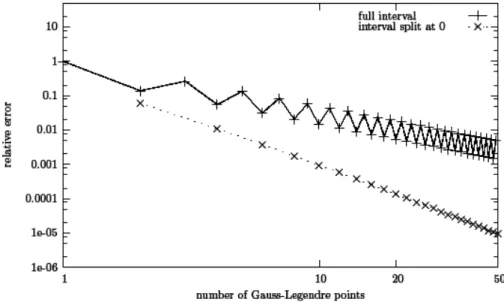
In the present section we analyze a very simple one-dimensional case in order to explain the problems we want to cope with in the more general case. Integration of a function over an interval using a Gauss-Legendre rule is known to converge exponentially to the exact solution if the function to integrate is regular (C∞). In our case, we are interested in the computation of functions with a singularity, or a singularity in one of their gradients, at the position of the crack tip. To start the analysis, let us consider the quadrature ofp(|r|) over the interval [–1 : 1], using Gauss-Legendre

points. Since the function has indefinite derivative at zero, the error in the integral does not converge exponentially. A first improvement would be to cut the interval at point r = 0 and perform a numeric integral over [–1 : 0[ and then

]0 : 1]. As can be seen in Fig. 3, in the first case, the error oscillates while slowly converging to zero with the number

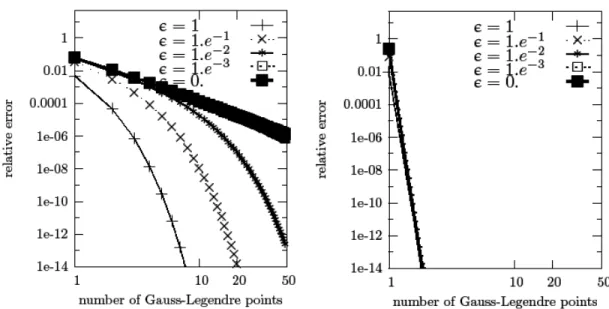
of points: in the second case, the convergence is still slow, but does not oscillate anymore. This first basic observation will motivate the choice of cutting the elements into cells that can contain the singularity only on their corner, not inside. Let us now pursue the analysis by considering the quadrature of√r over the interval [² : 1 + ²] with ² ≥ 0. On the left side of Fig. 4, we report the relative error of the quadrature of√x as a function of the number of

FIG. 4: Integration error ofp(krk) over [², 1 + ²]: (left) direct Legendre integration, and (right)

Gauss-Legendre integration after change of variable (2.1).

Legendre points used for ² ranging from 1 to 0. For large ², the quadrature rule converges exponentially with the number of Gauss points, but as ² goes to 0 the error becomes higher and higher for the same number of Gauss points. At the limit when ² goes to 0, the exponential convergence is lost and a very slow power law rate is obtained. The important point that we want to make is that in fact, as long as ² > 0 the convergence is indeed exponential, but as ² becomes smaller, one needs more and more points to see the effect of the exponential convergence. It appears linear. Of course the integral can be computed after a change of variable r = y2so that the integrand becomes regular on the full integration interval:

Z _b a √ rdr = Z √ b √ a 2y2_{dy (2.1)}

Numerical integration on the right-hand side then provides excellent results, since the exact result, up to round-off error, can be obtained with the two points Gauss-Legendre rule (see Fig. 4, right).

The difficulty in integrating the term of the bilinear form associated with the crack tip enrichment functions was of course noted in numerous papers (B´echet et al., 2005; Mousavi and Sukumar, 2010; Park et al., 2009) and are founded on a change of variable that cancels the singularity. But except in B´echet et al. (2005), only the cases where the singularity is at an integration cell vertex (and/or along an edge of an integration cell in three dimensions) are treated. In B´echet et al. (2005), a solution is proposed: a triangular cell is replaced by a superposition of three cells. Each of the cells has one of its nodes on the singular point, and the two others are two nodes of the original cell. The paper reports good results in this case, but this strategy implies the use of evaluation points that are outside of the original element, which limits its application and increases the total number of evaluation points. Outside the last mentioned strategy, we found no special treatment in the X-FEM or G-FEM literature applied to cells close to the crack tip, which do not contain the crack tip. If nothing special is done for those cells, the quadrature will converge very slowly. We propose here a new integration scheme, also based on a change of variable, but we extend it to the case where the crack tip does not coincide with a node of the cell.

In order to benchmark different integration strategies, in a first step we compute the stiffness matrix of one two-dimensional element and compare it with a reference solution. Let Ke_i be the stiffness associated with element e obtained using an integration strategy, and Ke_r be the reference matrix. In the following we use err as our error measure, where err = (kKe_i − Ke_rk∞)/(kKerk) and kAk∞= max{|aij|}. The reference matrix is obtained using an

adaptive integration scheme, built on top of the functiongsl_integration_qags provided by the Gnu Scientific Library (GSL) (Galassi, 2009). This function uses an adaptive algorithm to integrate a scalar function over an interval, until the estimated error is less than a threshold provided by the user.

3.2 Partition of the Elements

Starting with early X-FEM papers (Mo¨es et al., 1999), the elements are cut along the crack front into a partition of cells that does not cross the discontinuity, and then Gauss-like integration rules over the triangular cells are used. In this part we want to discuss the splitting strategies that produce the integration cells that form a partition of the elements so that each cell is in one of the quadrant of the crack coordinate system. This is the analog to what was just presented in our first improvement of the one-dimensional case.

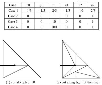
In the present work, we use the integration scheme over the triangle as can be found in Solin et al. (2004), where optimal rules over the triangle are given, classified by the polynomial order they can integrate exactly. We only used among these rules those which do not have negative weight nor point outside of the reference element. Table 1 gives the number of integration points for each polynomial order. For all the following integration benchmarks, the coordinates of the triangle nodes are given with respect to the crack tip coordinate system. The first results we want to discuss are results for which the crack tip are inside the element (case 1 in Table 2). The element is partitioned along the crack as in Fig. 5, according to lsnfor case 1a (Fig. 5, left) and according to lsnand lstfor case 1b. In case 1b, the element is first divided in three cells by triangulating the element, after a cut along lsn= 0, then each cell of the first partition is

TABLE 1: Number of integration points (nbpt) as a function of highest-order

polynomial integrated exactly over a triangle, following Solin et al. (2004)

Order 1 2 3 4 5 6 8 9 10 12 13 14 17 19

nbpt 1 3 4 6 7 12 16 19 25 33 37 42 62 73

TABLE 2: List of case tested for the different integration rule

Case x0 y0 x1 y1 x2 y2

Case 1 –1/3 –1/3 2/3 –1/3 –1/3 2/3 Case 2 0 0 1 0 0 1 Case 3 0 0 10 0 0 1 Case 4 0 0 100 0 0 1

(1) cut along lsn= 0 (2) cut along lsn= 0, then lst= 0

further triangulated after a cut along lst= 0. The goal here is to divide the element so that each cell is forced inside one of the quadrants of the crack coordinate system. Of course, this partitioning strategy is not the optimal one to achieve these properties, but it has the advantage to be built around the preexisting cut primitive to cut along the iso-zero of one level set. In case 1b, we therefore end up with a total of nine integration cells. With the last splitting strategy, a cell belonging to an enriched element can touch the crack tip with one of its nodes. In this case we call it a singular

cell, or the crack tip is strictly outside the cell and we call this cell a weakly singular cell.

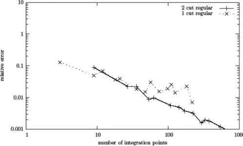
Error in the local stiffness matrix, as defined above, is plotted as a function of the total number of integration points over all the cells for the two cutting strategies as reported in Fig. 6 [For example, for the order 1 rule (one point per cell), we have three points in case 1a and nine points in case 1b]. In both cases, the convergence rate is slow. In case 1a (one cut), the convergence is not even guarantied; one can see that the error oscillates from one integration degree to the next. Even if the cut was not optimal (we integrate over nine cells), the error in case 2b is constantly less than in the case of one cut, at equal number of points. The convergence, while still slow in case 1b, oscillates much less than for case 1a. The previous experiment has been repeated for different relative positions of the crack tip and various element shapes, and it always shows an improvement when the elements are cut along lsn= 0 and lst= 0. This is related to the fact that by cutting the element twice, the singularity can only be on a vertex or strictly outside a cell. In the following, the integration algorithm using the second partitioning strategy and the regular Gauss-like integration rule over the resulting triangle is called partition integration and is parametrized by the order of the integration rule o used for each cell.

3.3 Treating the Singularity

As seen above, partitioning the element into a suitable partition of cells improves the situation by confining the singularity on a corner of a cell. For all elements in the enrichment zone, there are terms in the form of 1/r, 1/p(r),

p

(r), r which are singular or singular in their gradient for r = 0. In the literature, such singularity is already treated

properly for a cell which has one node on the singularity. In most cases, the authors used changes of variables before performing the integration that renders the integrand regular. Among those changes of variables, we concentrate on the one proposed in B´echet et al. (2005). First, a cell with a node on the crack tip is mapped via a linear mapping to a reference element that has the crack tip on its first node. Let us label ξ and η the coordinates in the reference element. Then the following change of variable is applied:

ξ = 1 2ρ

2_{[1 − sinh(τ)], η =} 1

2ρ

2_{[1 + sinh(τ)] (2.2)}

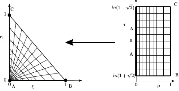
where ρ takes values in [0 : 1] and τ in {–ln[1 +√2] : ln[1 +√2]}. The change of variable defined in Eq. (2.17) can be seen as a map between the rectangle {[0, –ln(1 +√2)], [1, –ln(1 +√2)], [1, +ln(1 +√2)], [1, +ln(1 +√2)]} in the (ρ, τ) plane to the triangle [(0, 0), (1, 0), (0, 1)] in the (ξ, η) plane, as represented in Fig. 7. Note that the grid represented in the triangle is made of the isolines of ρ and τ. The singular point A in the triangle is the image of the line ρ = 0. This change of variable is very close to a polar change of variable, where τ plays the role of the angle and where ρ is close to the square root of the radius.

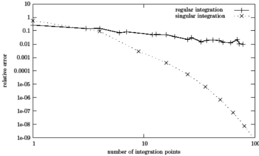
This change of variable was built with the previous consideration in mind and so that the domain that represents the triangle in the ρ, τ plane is a simple rectangle, where it is easy to build an integration rule by using a tensor product of Gauss-Legendre rule in each direction of the (ρ, τ) plane. This is exactly what is done in our next numerical experi-ment. We integrate the stiffness matrix for an element which corresponds to the reference element with the singularity at the first node (case 2 in Table 2), for different numbers of Gauss-Legendre points using the presented change of vari-able, and compare using regular integration points over the triangle. The one-dimensional Gauss-Legendre rules used to build the two-dimensional rules are rules starting at one point and ending at ten points. The number of integration points for the two-dimensional rules therefore range from 1 to 100.

Figure 8 reports the error in the stiffness matrix as a function of the total number of Gauss points. The results are of course much better using the change of variables. We can observe an exponential convergence rate. The error reaches a value of 7.28 × 10−9for 81 points and 7.406 × 10−10for 100 points, while the classic integration rule of highest order on the triangle just reaches 9.77 × 10−3with 79 points.

Unfortunately, even for the case where one node is exactly singular, the results are not always good enough. Even if the change of variable always improves the situation, the fact that the change of variable is done with regard to a reference element in order to always have a known rectangular domain on which to develop the integration rule can induce a relative loss of efficiency when the cell on which one wishes to integrate has a high aspect ratio (the shortest edge is much smaller than the longest edge), as can be seen in the following experiment. Cases 2, 3, and 4 from Table 1 are tested; they are all elements with the first node at the singularity, the third node at (0, 1), but the second node is at y = 0, and x is respectively set to L = 1, L = 10, and L = 100. The goal of the experiment is here to relate the aspect ratio of the cell to the accuracy of the integration rule. As can be seen in Fig. 9, the quality of the

FIG. 8: Error in stiffness matrix max norm for case 2, comparing regular integration with Gauss-Legendre integration

using a change of variable 2.17.

FIG. 9: Error in Stiffness matrix max norm for cases 2, 3, and 4: with a varying aspect ratio max(x)/ max(y) using

change of variable 2.17.

convergence is clearly degraded by the high aspect ratio. This point is, in fact, very important for the robustness of the overall method. Indeed, since the mesh is not related to the crack, the positions of the nodes relative to the crack type will dictate the shape of the integration cells. Even with a very-high-quality mesh, the cells can have a very bad aspect ratio. It happens if one node of the mesh is very close to the crack surface. Therefore, even for the case where one cell node is on the crack tip, the strategy proposed in most papers suffers from robustness issues even when using a special integration scheme of the type we just presented. But the situation in the particular case of a node on the crack tip, as we will show, is going to be improved by the general approach that we develop in the following.

3.4 Treating the Singularity for All Enriched Cells: the Algorithm

We have just shown that even when one node of a cell is on the crack tip, singular integration schemes are insufficient to get a rapid and robust convergence of the integration of the stiffness matrix. But perhaps more importantly, we also need to consider the case where the crack tip is outside of the element but still close to the element. This case is analogous to our one-dimensional analysis where the singularity was outside of the integration domain: even if the singularity is outside, the convergence rate is very slow if no change of variable is applied. So far, all the integration schemes that we used were found in the literature. In this section, we develop what we think is a new contribution to the field. After the discussion about the partition of the elements, we place ourselves in a framework where a cell is always in one of the quadrants of the crack coordinate system. Furthermore, we propose that a cell has to be in the positive quadrant (x ≥ 0 and y ≥ 0). If this is not the case, the cell is first mapped to the positive quadrant by reversing one or two of its node coordinates. No further mapping to a reference element is applied, contrary to the scheme presented in the previous section. Indeed, since the singular point can be outside of the element, there is no gain to apply any such mapping. We then consider the same change of variable but directly applied to a triangle in crack the coordinate system (positive quadrant).

x = 1

2ρ

2_{[1 − sinh(τ)], y =} 1

2ρ

2_{[1 + sinh(τ)] (2.3)}

The domain that represents the triangle in the (ρ, τ) plane can have a variety of shapes. If no node is on the crack tip, the shape in the (ρ, τ) plane is a curved triangle. When a node of the triangle is continuously moved to the crack tip, the curved triangle looks more and more like a quadrilateral with one straight edge on ρ = 0 at the end of the motion. Figure 10 gives some examples of the effect of mapping for some typical cell.

We now wish to integrate the stiffness matrix after having performed the change of variable by mapping Gauss-Legendre points on the unit square to the triangle in the (ρ, τ) plane. Fortunately, in order to perform this task, we can count on some properties of the change of variable. First, the change of variable can be inverted for all points but the

-1 0 1 0 1 1.4 -1 0 1 0 1 1.4 -0.8 0 0.2 0 1 2 -0.8 0 0.8 0 1 2 0 1 2 0 1 2 0 1 1.4 0 1 1.4 0 1 0 1 0 0.2 0.4 0.6 0.8 1 0 1 y τ ρ ρ ρ ρ x x x x τ τ τ y y y

FIG. 10: Effect of the change of variable (2.3) on some cells. Top: cell in the (x, y) plane, Bottom: corresponding

singular point, which means that by knowing the coordinate x, y of a point in the (x, y) plane, the coordinates ρ, τ can be computed as ψ−1_{: (x, y) → (ρ, τ) x ≥ 0 y ≥ 0 x + y > 0, ρ =}√_{x + y, τ = arcsinh} µ y − x x + y ¶ (2.4)

Let us now consider a segment [AB] in the (x, y) plane. This segment is mapped on a curve on the (ρ, τ) plane, for which the graph and its derivative can be computed. Let αAB, βAB, and γAB be three constant values computed as

follows from the coordinates xA, yAand xB, yB:

αAB= (xA+ xB)(yB− yA) − (yA+ yB)(xB− xA) (2.5)

βAB = xA− xB− yA+ yB (2.6)

γAB= xA− xB+ yA− yB (2.7)

The segment [AB] is described by the following curve ρAB(τ) and derivative ρ0AB(τ) in the (ρ, τ) plane, if τA6= τB:

ρAB = r αAB βAB+ γABsinh(τ) (2.8) ρ0 AB= − 1 2αABρ 3_γ ABcosh(τ) (2.9)

Alternatively, it can be described by the curve τ(ρ) and derivative τ0(ρ) if ρA6= ρB:

τAB= asinh(−βAB/αAB+ αAB/βABρ−2) (2.10) τ0 AB = −2αAB βABρ3 1 p 1 + (−βAB/αAB+ αAB/βABρ−2)2 (2.11)

An important property of the curve ρAB(τ) is that it is monotonous in τ for all points of the segment [AB] in the

positive quadrant [respectively τAB(ρ) is monotonous in ρ]. It means that the curve representing one edge of a

triangle in the (ρ, τ) plane is increasing or decreasing, exclusively. This property will be used very shortly.

In a first step of our algorithm to build an integration rule over the image of the triangle in the (ρ, τ) plane, we first classify each edge [AB] according to the value of τ0_AB(ρ) along the edge. If locally τ0

AB(ρ) is in [–1 : 1], then the

tangent of the curve is labeled to be “along” the ρ direction; otherwise it is labeled to be along the τ direction. Since the curve for one edge is monotonous, only four situations can occur for the “direction” of the edge, depending on the value of τ0_AB(ρ) at the extremities A and B of the segment:

i. (τ0_AB(ρA) ∈ [−1 : 1]) and (τ0AB(ρB) ∈ [−1 : 1])

ii. (τ0_AB(ρA) /∈ [−1 : 1]) and (τ0AB(ρB) /∈ [−1 : 1])

iii. (τ0_AB(ρA) ∈ [−1 : 1]) and (τ0AB(ρB) /∈ [−1 : 1])

In case 1, the edge is said to be in the ρ direction, and in case 2, the edge is said to be in the τ direction. In cases 3 and 4, there exists one and only one point ab on the edge [AB], such as we have τ0_AB(ρab) = 1 or τ0AB(ρab) = –1.

We call this point a cut point, and it can be found easily by using any root solver. In such a case, the edge is split in two parts, each part with one properly defined direction, either ρ or τ. Therefore for any triangle, by eventually splitting each edge at most once, we can construct a list of at most six edge parts. Each edge part is aligned either in the τ or ρ direction. A number of cases depending on the alignment of each edge part in the (ρ, τ) plane can be recognized, but before pursuing, let us include the case where one node of the cell is on the singularity. In this case, the mapping from the (ρ, τ) plane to the (x, y) plane is not invertible for points on the line ρ = 0. The image of the singular point of a triangle is a segment in the (ρ, τ) plane along the ρ = 0 axis and its direction is τ. The two edges connecting the singular point produce two segments for which τ is fixed and therefore, their direction is ρ. Only the image of the third edge of the triangle is curved on the (ρ, τ) plane. This edge cannot have any singular point, and the previous formulas can be used with no change to choose its direction or split it and choose the direction of its edge parts if needed (see Fig. 11). We end up with a list of at most four edge parts in this case, and the algorithm beyond this point is the same for cells with or without one node on the singular point. To keep the discussion brief, let us first discuss a typical case as seen in Fig. 12. The triangle (ABC) is mapped in the (ρ, τ) plane. According to our splitting rule, the edge [AB] is split in [A ab], which is found to be in the τ direction, and [abB], which is in the ρ direction. The edge [AC] is split in [A ca], which is in the τ direction, and [ca C], which is in the ρ direction. From these five edges, we now want to construct a partition of the image of the triangle in the (ρ, τ) plane so that each subcell is a curved quadrilateral (or eventually curved quadrilateral degenerated to a curved triangle when two consecutive nodes are at the same position). But we do not want any curved quadrilateral, we want quadrilateral, so that when traversing the contour-connected curved edge by the connected curved edge, the direction of edge 1 is ρ, edge 2 is τ, edge 3 is ρ, and edge 4 is τ. By imposing these conditions, we end up with a curved quadrilateral, with each edge as much as possible aligned with the ρ, τ coordinate axis. In the case presented in Fig. 12, it is possible to obtain a partition in two quadrilaterals by constructing one more point: the point [bc], which is the intersection of the curve [BC] with the axis τ = τA. Note that this point is easy to obtain because we have an explicit equation for the curve [BC] in the

form of the ρBC(τ). The two curved quadrilaterals, respecting the direction condition and forming a partition of the

0 1 0 10 -1 -0.5 0 0.5 1 0 1 2 3 3.5 y x ρ τ A C B A1 A2 C B bc a2a1 a1b

st -1 -1 sb 1 1 -1 1 -1 1 A C A B ca bc bc ab -1 -0.5 0 0.5 1 0.4 1 1.8 A B C ca bc ab ρ τ tb tt (ρ, τ) = φt(st, tt) (ρ, τ) = φs(ss, ts) 0 0.5 1 1.5 2 0 1 2 3 C A B bc ab ca xcp ycp (xcp, ycp) = ψ(ρ, τ)

FIG. 12: Singular integration scheme.

image of [ABC], are now [A bc C ca] and [ab B bc A]. Each of these curved quadrilaterals can now be mapped on a reference square in the (s, t) plane. The details of the subcell construction algorithm for all the different cases is quite technical, would take a lot of space, and are not necessary to pursue the discussion. We prefer to directly distribute the code, which will be freely available upon request.

In the following, we call [A0B0C0D0] a curved quadrilateral in the (ρ, τ) plane, with edge [A0B0], [B0C0], [C0D0], and [D0A0] respectively in the ρ, τ, ρ, and τ direction, with the the previously defined meaning. This quadrilateral is mapped to a reference square in the (s, t) plane, such as A0, B0, C0, and D0are, respectively, the image of (–1, –1), (1, –1), (1, 1), and (–1, 1) by ρ = 1 2(1 − s)ρA0D0(t) + 1 2(1 + s)ρB0C0(t) (2.12) τ = 1 2(1 − t)τA0B0(s) + 1 2(1 + t)τD0C0(s) (2.13)

where the functions ρA0_D0(t), ρ_B0_C0(t), τ_A0_B0(s), and τ_D0_C0(s) need to be defined. We detail the construction of

τA0_B0(t) in the following; the three other functions are constructed in a similar way. First note that by construction,

edge [A0B0_{] is aligned with ρ, following our definition — τ}0

A0_B0(ρ) is in [–1 : 1] and cannot change sign being either

positive, negative, or identically zero. If the slope is identically zero, then τA0_B0(s) = τ_A0 = τ_B0. Otherwise, we

first define ρA0_B0(s) by mapping linearly [–1 : 1] to [ρ_A0 : ρ_B0]. Then we set τ_A0_B0(s) = τ_A0_B0[ρ_A0_B0(s)]. This is of

course always possible since the curve is monotonous. This mapping is reproduced in Fig. 12. A square in the (s, t) is mapped on each of the curved quadrilateral subcell of the image of (ABC) in the (ρ, τ) plane. On this figure the grid is defined on the square of the (s, t) plane and is successively mapped on the (ρ, τ) and (x, y) plane, from right to left. It is now easy to construct an integration rule: For each quadrilateral in the (s, t) plane that forms a valid partition of a cell, construct a Gauss-Legendre rule which is a tensor product of classic one-dimensional rule. Then compute the coordinate of each point in the (x, y) plane by chaining the mapping and the change of variable. The overall algorithm can be summarized as follows, for a given triangular cell:

i. Compute the direction of each edge in the (ρ, τ) plane. ii. Split edges that need it at the point τ0(ρ) = +1 or –1.

iii. Divide the cell in “aligned” curved quadrilateral.

iv. For each quadrilateral, construct a Gauss-Legendre integration rule using the mapping between the (s, t) and the (ρ, τ) plane.

Each of the steps of the previous algorithm, except for the second one, have been fully described. There are a lot of possible alternatives to achieve this second step, and the implementation can be tedious. The full description of the second step as we implemented it, for the sake of the tractability of the presentation, is not exposed in the paper. The code that constructs it, as mentioned before, will be given upon request to the authors. We present and analyze results of this integration scheme in the next section.

3.5 Treating the Singularity for All Enriched Elements: Some Results

First we show the convergence rate for the elements presented at the beginning of the section, and then we present a more global benchmark of the integration rule that tests the algorithm for a large quantity of elements.

3.5.1 Integration Error Over One Element

Cases 2, 3, and 4 were designed with various degrees of aspect ratio, as previously described to measure the integration error when an element or a cell was strictly singular. Results applying the new algorithm are displayed in Fig. 13 and are to be compared with the previous results using only the change of variable presented in Fig. 13. The results for case 2, which is the reference element, are exactly the same as results obtained using only the variable change. This is because no edge split is needed in this case and the integration rule produced is exactly the same. For cases 3 and 4, the results are greatly improved. For these two cases, the edge not connected to the crack tip is split in such a manner that the algorithm, as represented in Fig. 11 for case 3, produces three subcells aligned with the (ρ, τ) axis:

[A1, a1b, bc, a2a1], [a2a1, bc, C, A2], and [a1b, B, B, bc] (the last quadrilateral being degenerated to a triangle). This

explains the total number of integration points reaching 300 for the highest-order rule used (again, a 10-point one-dimensional Gauss-Legendre rule). The best rule returns an error as low as 1.87 × 10−11and 3.482 × 10−8for cases 3 and 4, respectively, to compare with the value obtained by applying only the change of variable: 8.235 × 10−5and 1.521 × 10−4, respectively.

Case 1, which was first used to compare the merit of two splitting strategies into cells, as can be seen in Fig. 5 does not produce only cells with one node on the crack tip but also produces cells that, in the second splitting strategy,

1e-10 1e-08 1e-06 0.0001 0.01 1 1 10 100 300 rel at iv e er ror

number of integration points

L = 1

+

+

+

+

+

+

+

+

+

+

+

×

×

×

×

×

×

×

×

×

×

∗

∗

∗

∗

∗

∗

∗

∗

∗

∗

∗

FIG. 13: Error in Stiffness matrix max norm for cases 2, 3, and 4, varying the aspect ratio max(x)/ max(y) using

have a singularity close and outside of the element. Applying only the change of variable is not practicable for those cells, but the new algorithm is applicable for all the cells. As mentioned before, the splitting strategy produces nine integration cells, and the new algorithm from these nine cells generates a total of 17 (ρ, τ) aligned subcells. This appears to be a lot, but as can be seen in Fig. 14, this is still an efficient algorithm: The error obtained applying the one-dimensional 10-point Gauss-Legendre rule (for a total number of 1700 points) reaches an error of 3.47 × 10−9, while the best partition integration (for a total number of 9 × 79 = 711 integration points) only reaches 9.015 × 10−4.

3.5.2 Integration Error Over an Unstructured Mesh

The experiment could be repeated for a lot of elements, with varying shapes and relative positions to the crack tip, but in the following we propose what we think is a better benchmark that tests at once for a great variety of elements. The elasticity problem is solved on a square that contains a straight horizontal crack with the crack tip at the center of the square (see Fig. 15). On the boundary of the square, the tension found by computing the stress of an exact solution for a crack in an infinite domain is applied. The exact solution of this problem coincides with the exact solution in infinite domain, inside the square. The square is meshed with an unstructured mesh, and the displacement field is discretized by using the tip enrichment everywhere, and only the tip enrichment, multiplied by the partition of unity. The only difference with classical benchmarks used to show the h convergence of the X-FEM method, as used, for instance, in B´echet et al. (2005), is that we use only the tip enrichment functions, and these functions are used everywhere in the mesh. In principle, if the integration of the bilinear form was exact and if the obtained system of linear equation was not singular, we should end up with the exact solution, since the exact solution is contained in the enriched finite element space we just constructed on our square. Our first experiments trying this strategy were unsuccessful when using what we call the classic scalar enrichment in the first part of this paper. Indeed, when using a weak integration rule on quite coarse meshes, we were able to obtain some results, with quite high error, but when the mesh was refined or the integration rule was improved, we often end up with a singular system of equations that we could not solve with a direct solver (in our case superlu, described in Demmel et al. 1999). Further analysis, and as was noted in B´echet et al. (2005) or Laborde et al. (2005), showed that the space obtained by using the four scalar shape functions, produces

1e-09 1e-08 1e-07 1e-06 1e-05 0.0001 0.001 0.01 0.1 1 1 10 100 1000 1700 rel at iv e er ror

number of integration points

Classic integration over cell

+

+ +

++

+ ++ +

+++ ++

+

×

×

×

×

×

×

×

×

×

×

×

FIG. 14: Error in stiffness matrix max norm for case 1, crack tip inside the element, using regular integration and the

(−1, −1) (1, −1) (1, 1) (−1, 1)

t_{= σex}n

FIG. 15: Sketch of the benchmark problem. Traction on the boundary of the square (arrows) is computed from the

exact solution of a straight crack in infinite media.

a more and more ill-conditioned stiffness matrix as the enrichment zone grows, to the limit of a singular matrix when the enrichment is applied on all the nodes. As will be shown, this is not the case with the vector enrichment shape function proposed in this paper. But to keep the presentation consistent, we still want to use the scalar enrichment to show the gain of an improved integration strategy. In order to do that, we will reduce the enriched space a little bit by keeping only the needed enrichment function to produce a space that still includes the pure mode I opening solution. This reduction will be used only for the present benchmark. The other experiment wil, of course, use the full scalar enrichment. The full tip enrichment space in the two-dimensional case is reminded in the following equation:

X i∈[1:2] X I∈Ntip X α∈[1:4] NI(x)Fα(x)EiaIαi (2.14)

The directions of the physical space are enriched with each of the four scalar enrichment functions. We reduce this space by using a space where only F1and F2are used in both the Exand Ey direction, while F3and F4are only applied, respectively, in the Exand Eydirection. The space of shape functions used in our benchmark, using scalar

enrichment function everywhere, is now

X

I∈N

NIF1ExaI1x+ NIF1EyaI1y+ NIF2ExaI2x+ NIF2EyaI2y+ NIF3ExaI3x+ NIF4EyaI4y (2.15)

This reduction of the space insures the presence of a pure mode I opening field and produces a regular stiffness matrix when all the nodes of a mesh are enriched. The problem is solved on a square aligned with the crack, with crack tip at (0, 0), the two opposite corners of the square at position (–1, –1) and (1, 1), respectively. The mesh is built using the Gmsh package (Geuzaine and Remacle, 2009; Remacle et al., 2007). Each edge of the square is divided in 20 equal sized segments, for a total of 560 nodes and 1038 triangles for the final unstructured mesh. With the space used, we end up with 3360 degrees of freedom, 1228 integration cells and 1805 sub-cells for the new integration strategy.

For this test, we define the error err to be the relative energy error norm defined as follows

err = sZ

Ωh

(σh_{− σ}e_{) : (²}h_{− ²}e₎

σe_{: ²}e dΩ (2.16)

This error cannot be computed exactly, since the fields to integrate are singular. We could have used our integration rule to measure the error. Experiment proved that this is not necessary, and instead, we used the simple partition integration rule, with order 5 (seven points per cell), to evaluate the error. The error is reported in Fig. 16 as a function of the total number of integration points used to compute the stiffness matrix. As can be seen, while with the partition integration the error converges very slowly and with oscillations, the new scheme displays an exponential convergence rate and reaches very small relative energy error. The best partition integration (order 19) gave an error of 7.2 × 10−4 for a total of 89,644 integration points, while the new algorithm gave an error of 2.99 × 10−5for a total of 88,445 points, and the highest order used (20 points in the underlying one-dimensional Gauss-Legendre rule) reached an error of 1.13 × 10−9for 722,000 points.

3.5.3 Adaptive Strategy

On a reasonable scale problem like the one we just showed, one can ask about the penalty of a new approach in total computation time. Indeed, for the partition integration scheme, the integration points are known and are the same in the reference cell for all the integration cells. While in the case of our algorithm, for each cell, subcells must be constructed in the (ρ, τ) plane, and the integration point positions are the same for each subcell only in the (s, t) plane. In the context of a classic finite element method, this would probably be an unacceptable price to pay. Indeed, all the shape functions in classic finite element method are defined on a reference element, and the evaluation of the shape function at each integration point can be done once and for all, in the reference element. Only the jacobian must be computed separately for each element. In the context of the X-FEM, the enrichment functions are defined as a function of the position of the point of evaluation in the global frame. There is no possibility to evaluate the shape function without knowing the coordinate of the node in real space. Whatever the method to construct the integration points, which can be viewed as a preprocessing step done once for a given mesh and given crack, the enrichment functions need to be computed at each integration point of each element. At equal numbers of integration points, the time to build the stiffness matrix is equal, whatever method is used to construct them. In our experiments, the time to construct the integration points was always so negligible compared to the rest of the solution process that we did not

1e-09 1e-08 1e-07 1e-06 1e-05 0.0001 0.001 0.01 0.1 1 10 3000 10000 100000 1e+06 rel at iv e er ror in en er gy n or m

number of integration points

Partition integration

+

+

++

₊₊

+ + ++ ++

₊

++

₊₊

+

+

+

×

×

×

×

×

×

×

×

×

×

×

×

×

×

×

×

×

×

×

×

FIG. 16: Relative energy error norm, for a computation on a full mesh using enrichment everywhere, using partition

even bother to save them from one computation to another. They are computed when they are needed by the assembly process.

Nevertheless, if we could achieve a similar accuracy as the one just presented with fewer integration points, we would get faster assembling process. In order to achieve that, we will need some sort of adaptive strategy. Indeed, experiments showed that even with a small number of integration points, the new integration strategy gives very high accuracy in the local stiffness for most of the elements of the mesh. Only a few of them need a high number of points. Unsurprisingly, those elements are usually the one close to the crack tip. The direction is therefore clear. We could adaptively set the number of points of the underlying one-dimensional Gauss-Legendre rule from one cell to another if we had some sort of a priori error indicator for constructed rule over a cell. Our experiments have shown that the error in the evaluation of the area of a triangle using our integration scheme was strongly correlated to the error in the local stiffness matrix. This error, when all the points are mapped to the reference element, is very easy to evaluate: just sum all the weight of the integration points and compare to 0.5, the exact area of the reference element. So, for each element, we construct all the subcells and then iteratively construct the integration points for an underlying one-dimensional rule of increasing order until a threshold in the relative area error is reached. The experiment is reported in Fig. 17, where the relative energy error norm is plotted against the total number of points, for our integration algorithm with or without adaptivity, on the previous benchmark.

For the adaptive version, we set our parameter so that the minimum and maximum number of points of the one-dimensional Gauss-Legendre rule are 3 and 49, respectively. For each point of the curve, we set a different value of the relative area error threshold, starting at 1.0 × 10−2, and dividing by 10 for each new point until we reach our minimum threshold of 1.0 × 10−13. As clearly shown, a huge gain in accuracy at equal number of integration points is achieved. The best reported adaptive result is reached for the smallest relative area error threshold of 1.0 × 10−13. The energy error norm is then 3.476 × 10−10for a total of 161,271 points, compared to the 722,000 points obtained without adaptivity for an error still 3 times higher (1.13 × 10−9).

The last version of our integration method is referred to as the singular integration in the rest of the text. The

sin-gular integration is parametrized by the minimum and maximum number of points in the underlying Gauss-Legendre

rule (minpt and maxpt, respectively) and the area error threshold (ae).

1e-09 1e-08 1e-07 1e-06 1e-05 0.0001 0.001 0.01 0.1 1 10 3000 10000 100000 1e+06 rel at iv e er ror in en er gy n or m

number of integration points New algorithm

+

+

+

+

+

+

+

+

+

+

+

+

+

+

+

+

+

+

+

+

×

×

×

×

× ×

× ×

×

×

×

×

FIG. 17: Relative energy error norm, for a computation on a full mesh using enrichment everywhere, using the new

3.5.4 Comparison with a Scheme that Properly Treats Singular Cells Only

Up to this point, we only compared our integration strategy with the quite crude partition integration. In the following we compare it with a more advanced scheme presented in Nagarajan and Mukherjee (1993) and Park et al. (2009), and apply it to our setting. We call this strategy polar mapping. In the polar mapping strategy, elements are split into integration cells in the same fashion as in partition integration. Weakly singular cells are integrated using one of the Gauss quadrature rules over the triangle, and singular cells are treated by using a the following ”quasipolar” change of variable

ξ = r cos2_{(θ); η = r sin}2_{(θ); (2.17)} where r takes values in [0 : 1] and θ in [0 : π/2] and again, ξ and η are the coordinates of a reference element, such as the singular node is mapped on (0, 0) in the (ξ, η) plane. The integration rule is then constructed using a tensor product of the one-dimensional Gauss-Legendre rule. The polar mapping strategy therefore has two controlling parameters: the order o of the integration rule in the weakly singular cell and the number npt of Gauss-Legendre points in each direction of the (r, θ) map. Figure 18 compares the results between the polar mapping strategy, the partition integration, and the adaptive singular integration, on the same test case. For the polar strategy, o is increased from 6 to 19, while npt is set to 20. One can see that the polar strategy is of course better than the partition integration. The error is much less for an equivalent number of integration points: 97,012 points for an error of 0.0014 is the partition integration case, and 91,606 points for an error of 6.57 × 10−5 in the polar mapping case. The adaptive singular integration with 86,704 points gives an error of only 6.52 × 10−9, 4 orders of magnitude smaller than the polar mapping strategy. An error of 1.42 × 10−5, slightly better than the best polar mapping, is obtained with 31,025 points, less than one third the number of points needed with the polar mapping. From the curves of the convergence of the polar mapping error, one can see that the error is not necessarily smaller when one increases the number of points. It does not seem to be the case with the adaptive singular mapping.

1e-09 1e-08 1e-07 1e-06 1e-05 0.0001 0.001 0.01 0.1 1 10 3000 10000 100000 1e+06 rel at iv e er ror in en er gy n or m

number of integration points Partition integration

+

+

++

₊₊

+ + ++ ++

₊

++

₊₊

+

+

+

×

× ×

×

×

×

× ×

×

∗

∗

∗

∗

∗ ∗

∗ ∗

∗

∗

∗

∗

FIG. 18: Relative energy error norm, for a computation on a full mesh using enrichment everywhere, using the

3.5.5 Robustness of the Scheme Compared to Polar Mapping

In order to measure the robustness of the integration rule with respect to the relative position of the crack tip within an element, we next perform the following experiment. We take the same setting as in the previous experiment, we select the element where the crack tip is, and we do the same computation for different positions of the crack tip inside the element. More precisely, we will gradually move the crack tip xtfrom the center of gravity xg of the element

to the closest point xcto xgon the boundary of the element. This experiment is parametrized by s ∈ [0,1], such as

xt= (1 – s)xc+sxg. In Fig. 19, left side, the previous parametrization is depicted. We performed the same experiment

as before, for different values of s, and measure the error in the energy norm using the polar mapping strategy or the singular integration. For this experiment, we took the best polar strategy used in the previous computation (o = 19,

npt = 20) and the adaptive singular integration scheme that gave the same order of magnitude in the error (minpt = 3,

ae = 1.0 × 10−7_{). The results of this experiment are depicted on the right of Fig. 19. In the case of the polar integration}

strategy, the magnitude of the error varies from a minimum of 1.2 × 10−7 to a maximum of 7.8 × 10−4, almost 4 orders of magnitude. This contrasts with the singular integration strategy, which returns an error varying only from 1.09 × 10−5to 1.41 × 10−5. This contrast can easily be explained. When the crack tip moves closer and closer to the boundary of an element, the integration cells of the element on the other side of the boundary are more and more close to the crack tip, and therefore closer and closer to singular. With the polar mapping strategy, those cells are integrated with the classical integration rule that gives worse and worse results, while with the singular integration strategy, the singularity is taken into account. We think that this is an important fact, never reported before in the X-FEM literature. If close to singular cells are not taken into account properly in the integration scheme, the error in the stiffness matrix is very much dependent on the mesh (more precisely, the relative position of the crack tip inside an element). Treating properly the singular cell only is not enough to insure the robustness of the stiffness matrix computation. This issue might be crucial in particular for crack propagation problems where one as no control of the relative position of the crack tip of the element.

This concludes, for now, our work on the integration scheme for enriched elements. Starting from an efficient integration rule for singular cells (the parabolic mapping), we extended it in this contribution to weakly singular cells. This new integration scheme is efficient and accurate on any element, whatever its position relative to the crack tip. We have shown in the end of this section that the scheme, at equal numbers of integration points performs better than the partitioning strategy and also gives better results than the polar mapping.

s

= 1

s

= 0

s

+

+

+

+

+

+

+

×

×

×

×

×

×

×

FIG. 19: Variation of the energy error with respect to the position of the crack tip. Left: parametrization of the crack