Computational techniques which simplify the correlation between steady-state and transient response of filters and other networks

DOCUIjT ROOU 36-412

COMPUTATIONAL TECHNIQUES WHICH SIMPLIFY

THE CORRELATION BETWEEN STEADY-STATE

AND TRANSIENT RESPONSE OF FILTERS

AND OTHER NETWORKS

E. A. GUILLEM

Technical Report No. 268 September 2, 1953

RESEARCH LABORATORY OF ELECTRONICS

Massachusetts Institute of Technology

Cambridge, Massachusetts

Reprinted from the PROCEEDINGS OF THE NATIONAL ELECTRONIC CONFERENCE

VOL. 9, February, 1954

Department of Electrical Engineering and the Department of Physics.

The research reported in this document was made possible in part by support

ex-tended the Massachusetts Institute of Technology, Research Laboratory of Electronics,

jointly by the Army Signal Corps, the Navy Department (Office of Naval Research),

and the Air Force (Air Materiel Command), under Signal Corps Contract DA36-039

sc-100, Project 8-102B-0; Department of the Army Project 3-99-10-022.

COMPUTATIONAL TECHNIQUES WHICH SIMPLIFY THE

CORRELATION BETWEEN STEADY-STATE AND TRANSIENT

RESPONSE OF FILTERS AND OTHER NETWORKS"

E. A. GUILLEMIN

Massachusetts Institute of Technology, Cambridge, Massachusetts

Abstract.-In some wave filter applications it is significant to know or to investigate the transient

response for the contemplated excitation as well as to control the pertinent sinusoidal steady-state transmission and rejection properties. In others we may need to consider simultaneously the tolerance specifications on the transient response as well as on the steady-state frequency response of the filter in its design. The difficulty involved in handling such specifications lies primarily in finding a reasonably simple way (computationally as well as logically) of correlating tolerances or errors in the time domain with their counterparts in the frequency domain. Formally, this correlation is expressible through use of the Laplace transform; but from the standpoint of computational ease and interpretive clarity this mathematical relationship leaves much to, be desired. The method proposed in this paper effects the desired correlation without integration, and in many cases the pertinent results can be written down by inspection. While not an exact method, it is a very much better approximation than some other approximate procedures that have previously been proposed. The same techniques also enable us to compute readily the minimum phase associated with a specified magnitude vs. frequency variation, and thus obtain a relatively simple and direct way of computing transient response from a specified gain or loss characteristic that is as accurate as need be and one in which the appropriate asymptotic character of the filter characteristic is properly taken into account.

I. TIME AND FREQUENCY DOMAIN CHARACTERIZATIONS OF NETWORK RESPONSE

The so-called system function or response function of a (finite, lumped, linear, passive, bilateral) network, which is a rational function of a complex frequency variable s -= + jo, and may be either a driving-point or transfer function, is interpreted physically as the complex ratio of output-to-input amplitudes in the sinusoidal steady state defined by s = jo. It is the transform of the associated time function; for s jo, it is the Fourier transform, and for any complex s, it is the

Laplace transform (if we do not imply the usual restricted interpretation of the latter which assumes that the time function is identically zero for t < 0). The time function has the physical interpretation of being the response of the pertinent network when the excitation is a unit impulse.

If we denote the time function by f(t) and the associated system function by F (s), then their interrelation is expressible by means of the well-known Fourier integrals

(1) f(t)

JF(jo,)

j t do,; F(jo) f(t) e- j t dt

27r

f

-Cc -CC

-We speak of F (j,) as characterizing the pertinent network in the frequency domain, while f(t) is its time domain characterization. The integrals (1) are the means for obtaining one of these modes of describing the network response from the other.

In the practical design of networks the desired response may be specified either by

'This work was supported in part by the Signal Corps, the Air Materiel Command, and the Office of Naval Research.

513

prescribing F(jw) or f(t). If F(jw) is the prescribed function, the problem is said to involve frequency-domain synthesis; if f(t) is specified, we are dealing with a time-domain synthesis problem. In order for the construction of a network to be possible, the function F(jo), which is the starting point for this construction process, must in either case be rational.

In frequency-domain synthesis where F(jo) is prescribed, it may be given to us in the form of a rational function, but more often it is specified graphically; and we, must first find a rational function which approximates these graphical specifications with acceptable tolerances. In time-domain synthesis we might in some rare instance be given an f(t) whose transform is rational, but usually we will be required to construct a rational function whose inverse transform is an acceptable approximation to f(t) . The procedure here may be to find first a time function f* (t) whose transform is rational and whose approximation to f(t) is acceptable, or from the transform

F(jo) of f(t), find a rational approximant F* (jo) whose inverse transform f (t)

is acceptable as a sufficiently close representation of f(t).

However we approach the time-domain synthesis problem, it is clear that we shall need to make use of the relations (1) in some form in order to relate tolerances in the time and frequency domains, one to the other. In the frequency-domain synthesis problem where this particular aspect of things does not enter, we may nevertheless collaterally be interested in the time-domain response of the network, and hence be obliged also to make use of one of the transformations (1). In such cases we may sometimes wish to go directly from the given graphical specifications for F(jw) to the impulse response f(t). It is then that we must resort to some form of graphical integration (with its attendant approximations).

II. SUFFICIENCY OF THE REAL OR IMAGINARY PART

OF A RESPONSE FUNCTION

In any of these manipulations, the integrals (1) are found to be computationally cumbersome, and the solution to some very elementary situations often turns out to be a tedious and time-consuming task. It is the purpose of this paper to point out means whereby much of this sort of tedium may be relieved.

First we make use of the fact that if we are dealing with an f(t) that is identically zero for t < 0 (in other words, one that is dead before t = ) then it will suffice to use either the real or imaginary part of F(jwo) and thus eliminate one troublesome feature, namely, the complex nature of the transform. Recognition of the sufficiency of either the real or imaginary part of F(jo) as uniquely characterizing an f (t) which is dead before t = O, is easy if we observe, after writing

(2) F(jo) =

F,(o)

+

jF

2(w)

in the first of the two integrals (1), that F1(o), which is even, determines the even

part of

f(t),

and that F(o), which is odd, determines the odd part of

f(t).

Since

f (t) is zero for t < 0, it is clear that its even and odd parts must cancel for t < 0,

whence it follows that they are identical for t > 0, and either part therefore equals half, of f(t) for positive t. Thus with the implication that f(t) is to be discarded for negative t and only evaluated for positive t, one obtains the transformation integrals

o oo

(3) f(t) - - 1FF(o) cos wt d; F1(w) - f() cos t dt

07' 0

_ __

Correlation Between Steady-State and Transient Response

in which F(o) is the real part of the transform F(jo) as expressed in (2). If we use the integrals (3) instead of (1) then the function which uniquely char-acterizes f(t) in the frequency domain, namely F1(to), like f(t), is also a real function

of a real variable, and we are rid of the nuisance of having to deal with a complex - frequency function while we are concerned with the correlation of time and frequency domain tolerances. The rational function in the frequency domain with which we seek to fulfill the requirements on a stated f (t) in the time domain, is F (w) instead of the complex F(jo), which we can readily generate by well-known methods once we have an acceptable rational function Fl(to).

The fact that F₁() contains all of the information in the complex function F(jo)

and hence logically determines f(t) uniquely and reversibly as the integrals (3) show, may also be seen in other ways. Thus it is evident, for example, that quite generally

1

(4) F₁

(o)

= Re[F(jo)] -=

[F(s)

+

F(- s)] _j_

since

F(-

s)

is the conjugate of

F(s)

for s - jo. Now if the associated f(t) is

dead before t = 0, then F(s) is analytic in the right half of the s-plane. [Recall that evaluation of the first of the integrals (1) through setting jo = s and using methods of complex integration requires for t < 0 that we close the path of integra-tion by a large semicircle in the right half-plane, and the necessary condiintegra-tion that the value of this integral be zero in general requires that the closed contour so formed shall contain no poles. Being dead before t = on the part of f (t) is equivalent to analyticity in the right half-plane on the part of F(s).] Now if F(s) has poles only in the left half of the s-plane, then F(- s) has only these same poles reflected about

the j-axis. Moreover, the residues of F(s) + F(- s) in the poles of F(s) are the

residues of F(s) in these poles; and so it is clear that if we are given the rational function F (c), which is equivalent to being given F(s) -t F(- s), we can

uniquely construct F(s) because we know the locations of its poles, and we can compute the residues of F(s) in those poles.

III. THE PROCESS OF CONSTRUCTING F(jo) FROM ITS REAL PART IS UNIQUE EVEN WHEN j-AXIS POLES ARE INVOLVED

It is ordinarily pointed out that we must make an exception to the uniqueness claim if F(s) has poles on the j-axis, for the contribution to F(o) due to such poles is identically zero and hence F1 (o) is the same whether F(jo)) has additional

j-axis poles or not. (For example, a pure reactance is said to have an identically zero real part for s = jo), and so we can add an arbitrary pure reactance to any impedance without changing its real part.) This attitude is incorrect, as the following simple analysis shows.

Suppose we consider the function

(5) F(s) )

r(s + a)

having a simple pole on the negative real axis, a units to the left of the origin. For s j we find

a o

(6) F(jo) -- _

(and so we have in t his + 2case and so we have in this case

·_I _I__ __~ _II_ _11 _ I _ _I(

a -w

(7) Fl(w) -- ) 2 +

if we set a = 0, the pole in the function F(s) as given by (5) becomes a j-axis pole, and F

(o)

in (7) appears to become zero. This latter phenomenon, however, is a mirage. F1 (w) in (7) does not go to zero for a = 0, but becomes a unit impulse, as may be seen by plotting it as a function of (w for a -~ 0 and noting that its peak value at o) - 0 is proportional to 1/a. The width of its pulse-like shape between half-peak value points is proportional to a, and the total enclosed area equals unity. As a becomes smaller and smaller, F1(w) has the form of a pulse that becomes taller

and narrower while enclosing the unit area independent of the value of a. Clearly, the limiting process a -+ 0 converts Fl(w) into a unit impulse located at to - 0.

Using the notation u(x) for the singularity function of order n (having the transform s), the unit impulse becomes u,(x), and we can say that the function

1

(8) F(s)

7rS when evaluated for s - jw reads

(9) F(jo) - Uo(o) - j

7ro

Similarly, a function F(s) having simple j-axis poles at o = + o with positive real residues a is given by

(10) F(s) - -a

7r s - s - too jO)o

For s = j:o it has the real and imaginary parts

(11) F,(o) = a[u ( - w,) + u (o) + o))]

and

2ao (o

(12) F₂(w) = X 2

7r 0)02 o2

The time function corresponding to the F(s) given by (8) is the step function of value 1/7r

(13) f(t) =- u-1 (t)

77r

while that corresponding to the transform (10) is recognized to be

2ao

(14) f(t) - _-1(t) X cos oot

7r

Thus if we consider F1 ()) and f(t) as a transform pair, related by the Fourier integrals

(3), we may say that an impulse in the frequency domain (occurring at o, = 0) corresponds to a step function in the time domain (occurring at t = 0); and a pair of symmetrically spaced impulses in the frequency domain yield a cosine function in the time domain (for t > 0).

The imaginary part (12) is recognized as being the reactance of a parallel LC circuit. According to our present interpretations, the impedance of such a circuit

(for s = jo) does not have an identically zero real part as is usually stated, but instead it has the real part (11) consisting of a pair of impulses. If we consider-impulses as legitimate components in the construction of real-part functions, then it is clear that we no longer need to exclude pure reactances as legitimate components

Correlation Between Steady-State and Transient Response

of impedance functions constructible from such real parts; and we may state without reservations of any kind that an impedance (or admittance or dimensionless transfer function) is uniquely characterized by its real part. Given that real part, inclusive of any impulses that it may contain, we can find the complex function; and this function is unique.

Concerning transfer functions in particular, it is significant to note that no such unique relation exists between this function and its magnitude. Thus the specification of the magnitude of a transfer function determines uniquely only the so-called mini-mum-phase transfer function having this magnitude. From a given magnitude function we cannot determine the associated impulse response in the time domain unless we invoke the condition of minimum phase shift. If there is no clue in the given physical data that implies a minimum phase-shift condition, then nothing at all can be done about finding the associated time function. This difficulty is completely avoided if we work with the real-part function, for it fixes the entire system function uniquely whether it be minimum phase or not, and we do not have to consider the latter question at all.

IV. GRAPHICAL CONSTRUCTION OF A TIME FUNCTION FROM THE REAL PART OF ITS TRANSFORM

Now let us discuss the method by which we can carry out the transformation from a given Fo(w) to its associated f(t), or vice versa. As a specific example, let us consider the F(ow) function plotted in Fig. 1 and suppose that we wish to use the first of the integrals (3) to compute the associated time function. For this real part we have chosen the function

(15) F

(oo) =

for 1 I

to

<

I

1 + tan4 o

zero, otherwise

Since analytic evaluation of the first integral (3) for this function would prove rather difficult, it is evident that we should resort to approximate integration by graphical means.

.0

0.5

Fig. -The real part, F(w).

0

Accordingly, we divide the function into rectangular elements as indicated by the . oppositely cross-hatched areas and assume that cos ot is essentially constant throughout

the width of any element and equal to its value at the center of that element. If the areas of the elements are respectively denoted by a, a2, a, . . . and their center

frequencies by o1, o, t3, . .., then this process of approximate integration leads to

__11_1 __ ·_

CI __ _ IllsP_C _sl I_

the time function

2

(16) f(t) - (al cos olt + a2 cos W)2t +

+.

an cos wot)

7r

where n equals the number of elements.

The approximation involved in this result is two-fold. First, the rectangular shape of each element leads to a step-like approximation to the function F1(w); and second,

the assumption that cos ot is replaceable by cos o)kt is equivalent to replacing each elementary pulse by an impulse whose value equals the respective pulse area, its point of occurrence being at the pulse center. Thus the function F () is seen to be replaced by the approximant F1- (o) consisting of a succession of n impulses as shown in the

bottom half of Fig. 1.

Of the two sources of error involved here, the one due to replacing pulses by impulses is the more serious, particularly for larger values of t. If the width of each pulse is sufficiently narrow, these errors may nevertheless be within tolerable limits, but the total number of terms in (16) will then become rather large and the computation of f(t) will be correspondingly cumbersome. The remainder of this paper will show how we can improve the accuracy in this sort of graphical integration process and actually decrease the number of terms needed to represent f(t).

To begin with, we observe that in the integrals (1) we can differentiate under the integral sign with respect to that variable, t or to, which is a parameter so far as the particular integration is concerned and thus obtain the well-known result that differen-tiation in the time domain corresponds to multiplication by jo in the frequency domain, while differentiation in that domain (with repect to jo) corresponds in the time domain to multiplication by - t. As a result of this property of the Fourier

integrals (1) we can rewrite them in the form

oo oo

(17)

(-

t)

f(t)

*-fF(l)(j)

Ejt

do);

jo2

F(joi) =/f(l)(t)

c-jt

dt

-CO --03

where the superscript (1) indicates that the function is differentiated once. We can repeat the process and have (- t) 2 f(t) expressed in terms of F(2' (jo,), or

(j) 2 F(jo)

in terms

of f(") (t),

and so forth.

In the same manner in which the integrals (3) are derived from (1) we can then obtain

00oo 00

2

f(t)

-

_rt

F()( ) sin t do); Fl(co) = o ( I (t) sin tot dt

o o

(18)

-

s

JF(2)

()t)

cos

wt

do; F

(J))

Cos

t d

t

o 0

and so forth. These relations are, of course, valid only so long as the integrals exist, but this question need not concern us at the moment. In these last results, differentiation of F () is with respect to o, not jo).

Let us consider that integral in (18) which expresses f(t) in terms of F1(1) (o)

Correlation Between Steady-State and Transient Response

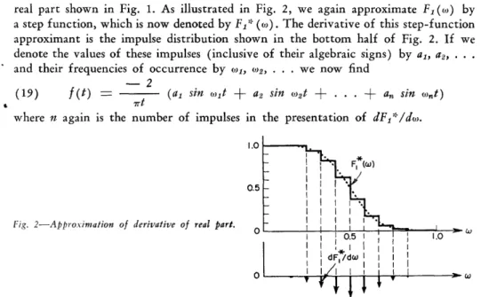
real part shown in Fig. 1. As illustrated in Fig. 2, we again approximate F (o) by a step function, which is now denoted by F₁* (to). The derivative of this step-function

approximant is the impulse distribution shown in the bottom half of Fig. 2. If we denote the values of these impulses (inclusive of their algebraic signs) by al, a₂, .

and their frequencies of occurrence by ol, o, ... we now find

-2

(19) f(t) = (al sin ) t q- a sin O2t + . . a,, sin ont)

7rt

where n again is the number of impulses in the presentation of dFl/d).

1.0

0.5

Fig. 2-Approximation of derivative of real part.

0

The important difference between this result and that expressed by (16) is that the only error committed is that due to the step approximation of F (o). The impulses are true impulses this time. The expression (19) is, therefore, equally good for all values of the time t. If we are willing to tolerate the same average error with our present approach as with the previous one, we can probably make a cruder step approximation (which need not, incidentally, involve uniform increments) and obtain an expression for f(t) involving fewer terms than before. This is the goal at which we are aiming.

We can continue to take further advantage of this sort of reasoning. Thus if we were to construct an approximant F* (o) consisting of straight line segments-a so-called piecewise-linear approximation to F(o)-then its first derivative becomes a step approximation and its second derivative a sum of impulses. For the same number of impulses as before, the piecewise-linear approximation to F(to) is much better than the step approximation; or for the same approximating tolerance we will now have still fewer impulses. The expression for f (t) is readily obtained from the appro-priate integral in (18). We are now in a position to generalize these ideas. In this generalization we will have no need to use any of the above Fourier integral relations. We will obtain all of the desired results in a simpler and more direct manner.

V. THE GENERAL METHOD OF DETERMINING APPROXIMATE INVERSE TRANSFORMS

The mode of approximation logically following the piecewise-linear procedure is one in which F1(o) is approximated by a set of confluent parabolic arcs. Thus a fairly

decent approximation to the Fl (to) function shown in Fig. 1 might consist of just two such arcs, confluent at the point to = 0.5, one with its apex at wo = 0 and the other with its apex at (o = 1. The first derivative of this approximant is a piecewise-linear approximation to the true derivative of F (to) and has just two break points:

(_1 IIII _LI I--·-11----· -C P-ill-·--·--- I-

one at w = 0.5 and another at = 1. It is the third derivative of this approximant which now consists of impulses (at the break points of the first derivative), and the corresponding time function is given by just two terms.

The time functions obtained in this way, like (19), contain powers of t in their denominators, but this fact should not be construed to mean that f(t) becomes infinite for t = 0. This item will be discussed later on in connection with the question of how the proper asymptotic character of F(s) is taken into account.

In the following generalization of these ideas we will not bother to distinguish the approximant to F1(o) by an asterisk. The vth derivative of this approximant we

will denote by F( )(o) and assume that it consists of a sum of impulses. If we remind ourselves that Fl (o) is an even function and hence that all of its even-order derivatives are likewise even, while all odd-order derivatives are odd, we see that the vth derivative of the approximant to the given real part is given by an expression of the form

(20) F,(l() =

a:

ak[0o(w - )k) + (-1)" Ito( + wk)]

k=1

By use of the reasoning that relates (10) and (11), noting also that

d/ds

=

d/jdo,,

we see that the system function having the real part (20) is (21)

F(" (s)

=

(j) ak - - + (- 1) S +

-k=1

where the superscript (v) here indicates the vth derivative with respect to s. To obtain the corresponding time function, we need merely remember that the transform of

es.tis 1/ (s - o), and that v-fold differentiation of F(s) corresponds to multiplication

of f(t) by (- t) . Thus the time function corresponding to the real part (20) is

seen to be given by

(22) -2

()

-2-

) 2

eak

cos okt, for v even

(22) R0 - 7rtv

k~l

and by

.(23 ) f M = 2 (- ) (+S)/2 v

=The

questions that are uppermost in one's mind at this point are: What is a1 The questions that are uppermost in one's mind at this point are: What is a good procedure for determining the values of the coefficient adk in a given situation, and how does one decide upon a value for the integer v? The relevant factors involved here are best seen in terms of a specific example, and so we return once more to the real part shown graphically in Fig. 1 and given analytically by (15). In Fig. 3 we have plotted this function again, and below it the first and second derivatives. We might remark that successive differentiation clearly accentuates the variable properties of a function. While the given real part is exceptionally smooth (it was chosen for this reason), its second derivative is rather jagged in character and differs very little from the broken-line approximation (shown dotted).

Correlation Between Steady-State and Transient Response 1.0 0.5 0 0 -0.5 -1.0 1.5

Fig. 3-Fl(w) and first two derivatives.

1.0 0.5 0 -0.5 -1.0 -1.5

If we thus approximate the second derivative of the given real part, then its first derivative becomes approximated by parabolic arcs, and the approximant to the real part itself consists of third-degree parabolic arcs. The fourth derivative of this approximant consists of a sum of impulses; in the formulas (20), (21), (22), and (23), the integer v equals four. Since the broken-line approximation in Fig. 3 has four break points, there will be four terms in expression (22) for f(t).

A less good approximation to the given real part will result if we use a broken-line approximation to the first derivative with the same number of break points. Such an approximation to Fl(l) (w) in Fig. 3 would be trapezoidal in character. A simpler one, triangular in form, would do almost as well and would involve only three break points and hence only three terms for its time function representation. In either case we would have v = 3; that is, the third derivative of the approximant to the given real part (consisting of two confluent parabolic arcs) is a sum of impulses.

It is significant that a piecewise linear approximation of F) () with four break points offers little improvement over the one with three, so far as closeness of approximation is concerned. If we are willing to use four terms in the expression

W

OJ

1.0 -W

_

IC 1 __III__I_____I_______II___ C _

for f(t) then we should use the piecewise linear approximation to F1( 2) (() as pointed

out above, for this one will yield an approximant to F (to) that is much better than the ones obtained from a similar approximation of F,(l) (o) with either three or four break points. We can obtain a still better degree of approximation by considering the third derivative of Fl (w) and approximating it by a broken line. However, the third derivative has an additional change of sign and will require a broken line with at least five break points. Hence, we will get this better approximation to the given real part at the cost of one additional term in the representation for f(t).

VI. ERROR ESTIMATION

If a certain derivative of the given real part, like F(2) () in Fig. 3, is approximated

by a broken line, the question is to estimate, from this approximation, how closely the given function is approximated. For example, in Fig. 3 we can readily measure the maximum error between the broken line and the true second derivative. From this value, we wish to determine the maximum tolerance between the given function and the approximant whose second derivative is the broken line.

In Fig. 4 we show the approximate behavior of the error between the broken line in Fig. 3 and the true second derivative. We note that the error changes sign three times along any straight line segment (of the broken line in Fig. 3) and that the number of segments is one less than the number of break points. Hence, if the number of break points is n, then the error involved in the broken line approximation will ordinarily change sign 3 (n- 1) + 1 times.

g 0.10

-\ 1

-00 xI i o i oI

I.

' Fig. 4-Error in broken line approximaton.

.- oo.10

Since the function F1,( ) is approximated by impulses, F₁(l- 2) is the one that is

approximated by a broken line. In order to get an estimate of the error between the given real part and its approximant, suppose we assume that the break points are equally spaced and that the maximum deviation between the broken line and F1(P- ;)

is uniform and equal to . Then the approximate plot of the error, as in Fig. 4, would have the form of identical alternately positive and negative triangles whose common base is

(24) n

1

3(n -

I) + 1

since we are taking the width of the entire approximation interval equal to unity-a normunity-alizunity-ation thunity-at cunity-an unity-alwunity-ays be munity-ade.

The integral of this error function is again oscillatory with a maximum deviation from the mean equal to the area of a triangle which is the

(25) error in F1( - s) = (a)

2

If we assume that the corresponding error curve again has an essentially triangular character and apply to it the same reasoning that has just been applied to the initial error, we obtain the

Correlation Between Steady-State and Transient Response

(26) error in F'( -4) -= (- )2

Continuation of this process yields the

(27) error in F1 = 2()-2

which is an optimistic value for several obvious reasons, but perhaps is sufficiently close for estimating how far we should go in forming successive derivatives (that is, how to choose the integer v) in a given problem.

If we apply this method of error estimation to the problem illustrated in Fig. 3 in which F(2) is approximated by a broken line, we have: n = 4, v = 4, and by (24),

8 = 1/10. By inspection of the figure we see that E is about 0.1, and so (27) gives 1

(28) error in F -= 0.1 X (- ) 2 = 0.0004

20

Since two or three times this value is still a pretty small error we see that the results obtained with four terms in this example should be rather close. In any case, one can always compute the approximate error in the approximation to F₁(oh) and convert

it into a time function by the same process in order to determine the corresponding error committed in the time domain.

VII. ASYMPTOTIC BEHAVIOR

From established properties of Fourier and Laplace transforms we know that if

F(s) behaves like l/Sk for s -+ co, then f(t) behaves like tk -l for t -+ 0. For

example, a step function has the transform 1/s; a linear ramp function has the transform 1/S2, and so forth. It is not as well known but readily established that if

for - c

I 1 1

F(jo) -+ , then F(o) -2 and F(,,)

} o o,3 ,

if

I 1 1

(29) F(jo) -+ , then F(o) -- and F2(o)

-if

I 1 1

F(jo) - O -, then F(,o) --+; and F (o,)

and so forth.

For a given asymptotic behavior on the part of F(s), the real and imaginary parts for s = j,) have a definite asymptotic behavior. Specifically, F (o)) will always ultimately drop off as the reciprocal of some even power of o, and F₂(,) as the reciprocal of some odd power. In the foregoing plots of F₁(o)), such asymptotic behavior

was ignored completely. In fact, the function was assumed nonzero over only a finite frequency interval which we normalized as 0 < w < 1. While this assumption may seem justified in view of the fact that F(o)) must become small at least as fast as l/o2 for large w and hence will have negligibly small values beyond some finite upper frequency limit, we cannot be sure that the process of chopping off the asymptote of this function might not introduce some troublesome error, and so it is necessary that we find a way of controlling this aspect of our problem.

I_ _I_ 11 __II_1__________IIYf--·ll···l1-·lp-·

The starting point in this discussion is the vth derivative of the system function given by (21). This expression is actually the partial fraction expansion of F(V) (s), and + ak are the residues (apart from the factor 1/7r) in its j-axis poles. Suppose we also consider the corresponding partial fraction expansions of the functions sF(v) (s),

s2F(v) (s), s3F(v)(s), and so forth. These all have the same poles as F(v) (s) but

with altered values for their residues. In the pole at s - jok, the residue is ak(jok) P,

and in the pole at s = - jok it is ak(- 1)v (- jo))P. For p = 0 these are the residues of F( )(s) as given in (21), and for p = 1, 2, . . . they are the residues of the other functions in the above-mentioned sequence.

We now make use of a well-known theorem in function theory which states that if a rational function of the complex variable s behaves for s -+ like /s" with the integer q 2, then the sum of the residues of this function is zero. If we regard sF (")(s) as being the function in question, then this theorem yields the

result that

(30) E [a,(jo)) + ak(-l) (-jo)v) ] 0 for q 2

kI=1

This result is obviously trivial for p + v = an odd integer, but for p + v = an even integer we have

n

(31) E ak,;,.P 0=

k=l

If v is even, p = 0, 2 ... ; and if v is odd, p = 1, 3,...

Now let us see about the condition q 2 for which this result is true. Suppose the system function F(s) for s --+ oc behaves like 1/sk. It is then clear that its vth derivative behaves like /sk +" and so we have k- + v = p + q, and our condition becomes q k + v - p ' 2, or

(32) p k- + v- 2

For example, if the asymptotic behavior of F(s) is like 1/s3 and v = 4, then

k +- -2 = 3 + 4 -3- 2 = 5, and the condition (31) holds for p = 0, 2, 4,

It is useful to see what these conditions mean from several other points of view also. Thus from the representation for the vth differentiated real part given by (20) we can obtain the corresponding expression for the ( - r)th differentiated real part, namely

(33) F₁l(,-r() = E ak[u(o-) - (- 1)v Ul-r() + )k)

k=1

If we evaluate this expression for = 0, only the second term in the bracket is nonzero. Hence

(34) Fl(v-r)(O ) = E (_ ) v alU-()k) k=l

From the fundamental definition of the singularity functions we have, however,

(35) Ur(wk)

(r - 1)! Substituting in (34) and letting r- 1 p, we have

(36) akto)kP = (-I )v P! F(v-P--l)(0) k=1

Correlation Between Steady-State and Transient Response

If we remember that F(o(w) is an even function, but that all of its odd-order derivatives are odd functions and hence are zero for o) = 0, we have the result (31) again with its specification that p is even when v is even, and odd when v is odd, because v - p - I must be odd.

This method of deriving the result (31) does not yield the range of p-values for which it is true, but if we make use of the result (32), we find that (36) holds for

(37) (v - p -

1)

I , - k - v + 2 - I = I - k

For k > 1 this is a negative integer, which implies successive integrations of the real part F(o).

The left-hand side of (36) for p = 0, 1, 2, ... represents the moment (of corresponding order) of the impulse distribution about = 0. We shall refer to

(31) or (36), therefore, as moment relations.

Of special interest is the particular condition (36) for v - p - 1 = 0, which reads

(38) ak - ' = (-1) (v- 1)! F₁(O)

7=1

It is always advantageous in numerical work to normalize the amplitude of the function

Fl (o)) by setting its zero-frequency value equal to unity (as is done in Fig. 1). This

normalization process thus fixes one of the moment values, and together with the relations (31) forms a set of requirements to be fulfilled by the as that are referred to hereafter as the moment conditions.

Let us now see what these moment conditions mean so far as the time function given by (22) and (23) is concerned. If we replace the cosine and sine functions in these expressions by their Maclaurin series, we find

(39) 2 (- 1) //2 ak akOJk 2 akwk4

f(t)

_{7r 1 1}

t

-

₂

2!tv-

_!t,-2

+

_4!t"-~

t-l

-

. .

for v

even Ic=l and

(40)

2 (-1)

± 1)/2 ako)k jakwk ak)k5

f(t) = _-r -+ _... _{3!t 3} - for v odd

5

k=1

The moment conditions (31) for p-values satisfying (32) are now seen to assure that these expressions behave properly for t = 0. Thus so long as the moments are

zero for v - p I, f(t) will not become infinite for t = 0. Since p iv - 1 is surely contained in the values allowed by (32), even for k = 1 which permits f (t) to have a discontinuity at t = 0, we see that the results (22) and (23) are guaranteed not to "blow up" for t = 0.

We notice, incidentally, that the Maclaurin series (39) and (40) contain only even powers of t. This is to be expected, since the time function obtained from the real part of F(jo) must be even. For this reason we cannot expect our present results to reflect correctly the asymptotic behavior F(s) -+ /sk for k/ equal to an even

integer because the Maclaurin expansion of f (t) in such a case should begin with an odd power of t.

) _ I_ I _ _ _ _ I C_ 1_1 s I I _

This circumstance is, of course, of no great moment. In fact, this whole question regarding asymptotes and how to take them into account should not be taken too seriously. So long as the time function has roughly the right behavior in the immediate vicinity of t = 0 we need not have any further concern about chopping off an asymptote, since the behavior of f(t), except in the very immediate vicinity of t - 0, is no longer controlled by such an asymptote but rather by the form of F1(o) over

that range of frequencies where it has appreciable values.

If we nevertheless insist that f(t) should correctly reflect the asymptotic behavior of F(s), then for even integer values of

k.

as defined above, we should derive f(t) from the imaginary part of F(jo) rather than from its real part, for then f(t) will be an odd function and its Maclaurin expansion will contain only odd powers of t. For this approach we represent the vth derivative of the imaginary part F₂() as a sum of impulses, and have instead of (20)

n

(41) F2()(o) = a, [o(o - o)k) - (- I) Uo (' +

1

o)k)]

k1c In place of (21) we find n (42) F(v)(s) aL - -

(

1) r(i₎ LS - jo)k + j,)k k=l

and for the time function we have

(43) 43)

fM(t=

t) = -- 2t 7rtv L

a,,

ak cos okt OS

for

for v odd

v

odd

k=1

and

it

2 (- 1)( + 2) /2/

(44) f(t)

=

ak sin (Okt for , even

k=l

We can thus work with the imaginary part in essentially the same way as was discussed for the real part above. Except for this question of asymptotic behavior, however, there is little choice between working with the real or with the imaginary part of F (jo).

In order for the reader to get a better idea of how the moment conditions enter into the solution of a problem, suppose we consider a real part function having the general character of the one shown in Fig. 1, and for which the asymptotic condition

F(s) -+ I/s for s -+ o is to be met. In order to fix things further, suppose we

decide upon an approximation of F(o)) by means of parabolic arcs so that v = 3. The relation (32) tells us that we have only one moment condition (31) to fulfill, namely for = 1, while normalization of the amplitude of F(0)) requires (38). Thus we have in this case

(45) n ak o)k 0= k=l and n ' ak o = -k _ 2 k=l

Correlation Between Steady-State and i ransient Response 527

frequency ovl between zero and one. The broken line approximation of f13l) (o,) then has two break points: at o = ol and at o = 1. The moment conditions (45) read

('6) a l 4+ a = 0

a_l (l +- a₂ = - 2

In this simplest case, the moment conditions fix everything as soon as the point of confluency i), is chosen. Suppose we let o) = 0.4. Then (46) gives

25 10

(47) al - , a -- -_

3 3

The approximant to the given real part becomes

(48) F1(w) = - -) - US(w +

-

)

-_ -__(_ - 1) - l.3()

-4+

1)

]

If we want to plot this function to see what it looks like, we have

25 2 10

6 5 6

while for 0.4 < w < I we must add the term [25/6] [o - (2/5) ]2. After

simplifica-tion we have

(49) F(o)

=

.1 ₅

-_

-w ₁₀ for 0 < ₅ -< 0.4 °

3

3

3

This function as well as its first three derivatives are plotted in Fig. 5. The time function is immediately written down, using (23), thus_{25 100}

2 sin 0.4t - sin t

- - ) - )' for 0 < o.

5 67r

It contains a step at = O, as required by the assumed asymptotic condition. As a second example let us choose the asymptotic condition F(s) -O- 1/s8 and again use the parabolic arc approximation so that ' = 3. According to (32), the

condition (31) applies for = 1, 3. Together with the normalization (38), this ives

E al; 0)7i = 0 k=l tion we have * (51) F I, o for 0 a - 2 FI, - ) (

a

- (

0

or 0.4 < 25 sin 0.4t sin t k I -- k=l -- I I L -- I-- -

I---1.0 0.5 0 0 -I -2 4 2 0 -2 -4 0 F. It"u point of 'confluency w l - (2 ) I F,(2)M _(3), . W) c) 3 C w CU o,

Fig. 5-Real part for example 1. Fig. 6-Real part for example 2.

The simplest approximation will involve three arcs, and the pertinent a-values must satisfy the equations

(52)

a,

o,, + a₂ o)2 + as - 0

al tol S

+ a2 23

+

as = 0

We now have only to choose the break points. Suppose we let o) -= 1/3, 0)2 = 2/3.

Then (52) yields

(53) a, = 45, a2 = - 36, a = 9

The real part function which these ak-values imply is found to be

- ! -2 -k -I 1-1 I I I I v T c I

Correlation Between Steady-State and Transient Response F(oW) = 1 _ 92 for 0 < <-7 27 1 2 (54) - -o) 15 +

_

2o for - < <

-2 2 3 3 9 9 2 F1() - - -+ 9 - - o' for - < < 1 2 2 3

Plots of this function and its first three derivatives are shown in Fig. 6. As required by the assumed asymptotic behavior, the real part has one change of sign, and encloses zero area, which, according to the relation (36), is the meaning of the third condi-tion (51).

The time function is obtained from (23) to be

(55)

₂

t

2t

2 ()= 45 sin (-) - 36 sin (-) + 9 sin t

/ (t)

_7r

-

-

t~

_t3

7r 27 729

from which we see that the proper behavior at t = 0 is obtained.

These examples show that fulfillment of the moment conditions as required by the pertinent asymptotic behavior and the amplitude normalization of F (o,)) curtails to some extent the ability to approximate arbitrary functions with a limited number of terms. This result is, however, entirely logical, since the added requirement of meeting certain desired asymptotic conditions can only be met through relinquishing some other desired features or increasing correspondingly the total number of adjust-able parameters.

VIII. TRANSFORMATION FROM TIME TO FREQUENCY DOMAINS

Esszntially the same methods may be used to find the real and imaginary parts of

F(jo) from a given time function. Thus if the vth derivative of f(t) is given by

a sum of impulses for t > 0, then f(t) itself has the representation

(56) f(t) ak u_ (t - tk)

Since _ (t) has the transform s-V, and delay of a time function by t seconds amounts to multiplication by -jw'k in the frequency domain, we see that the transform of the function in (56) is

(57) F(jo)) a,

k=l

having the real and imaginary parts n

(-1 )v/2

(58) Fi(o) a COS tot_k for v even

k=1

II __ _ _ _ C I_ _ _ _ _C _ II _ _ _ _

n

(59) (

+

')/

(59) F,(t)

(

( ak sin tk for v odd kc=i

and

n

(60) (I+1)/2

(61) F2() = ak cs o)t for v

oddeven

k=l

(61) F2(W) -cos t for odd

IX. APPLICATION TO PHASE DETERMINATION

As pointed out in Sec. III, the magnitude of a transfer function for s - j, does not uniquely characterize that function and therefore does not determine the pertinent time function unless we specify that a minimum phase shift is to be associated with the stated magnitude. When a problem of this sort arises, it is necessary first to find the minimum phase function compatible with the given magnitude. When the phase is determined one can readily compute the real part of the transfer function and from it the impulse response as described above. We wish now to show that the same techniques may be used to obtain the phase from a given magnitude in an analytically closed form which lends itself to numerical computation far more readily than do the presently known procedures for accomplishing this same end.

Our starting point in this analysis is (9) which shows that the imaginary part associated with a unit impulse real part is -I/ro. If a sum of impulses represents the tfh derivative of a given real part, then the associated imaginary part is a cor-responding sum of the vth repeated integral of -1/7ro). It is convenient to write the sequence of successive integralsb

I I (62) vo(o) - -7r to 1 (63) v_l() - In o2 27r 1 (64) v_ 2() - - (o In o 2 - 20,)) 27r (65) Vs() -

--

(

_

In _ 2 o

)

( In 2 (66) V 4(-) = - _o? - 18

)

27r 6 18

which are the imaginary parts associated with a real part equal to u (o) for v= 0, 1, 2, 3, 4,

The system function or response function is now represented in the exponential form

(67) F(jo) - e-(a+i#)

bSince (9) comes from (7), we should integrate (7) and then set a - O. If we do this it becomes

clear that InX/w2 can be written In! w but not as Inw.

Correlation Between Steady-State and Transient Response

in which a((w) and A (o,) are the familiar loss and phase functions expressed in nepers and radians respectively.

In terms of the preceding method these functions have the representations

(68) a () -= ak

-1;= [u_ (o - ok) + (-1)v U_ (° - + k)]

(69) /(ow) - ak [V_ ( - k) + ( I) v_ ( + Ok)] k=l1

Evaluation of /3(w) through substitution of the pertinent expressions for v_ (w) is simplified if we observe that the second terms in the right-hand members of (64),

(65), (66) and the following ones in this sequence contribute nothing and may

therefore be dropped. To appreciate the truth of this statement, note, first, that these terms introduce into the sum (69) the following expression

(70) ak[ - k)p-I + (- 1) (W + -k) - ']

If v is even, the bracket yields terms involving only even powers of o)k up to v - 2; and if v is odd, only odd powers of fok up to v - 2 are present. If we make use of

the relation (36) with a(o) in place of Fl(wo) and note that odd order derivatives ale odd and hence

(70), the value of for the phase

are zero for o - 0, we see that for the powers of wOk present in (36) is zero and hence (70) equals zero also. Thus we may write

1 (71) /3(w) -- - ak[ ( 7r i k=1 - ok) in Io - O)kl + (,) + O)k) In 1 + - kl] for v - 2 (72) () =-1 = ak (' k=l - Wk) 2 In [) - Wki -() + ()k)2 n In + (ki] for v = 3 n (73) f/3() - ak[ (o 67r k=l and so forth.

It is helpful to have an expression fo

- )k) In IW - [kl +

(W) + Ok)3 In + o)k|] for

v

-4

r the phase valid near o) = 0. Evaluation of the linear term in the Maclaurin expansions for the above functions leads to

, (75)

(76)

( ) - a k In eok + . . . for v

=

2

k=l n

t3(o) = - o akk In olk + . . . for v = 3

7r k=1

_ _ I _ I _ I I_ y_ _ C----·l _ ----I

-20 k2

(77) -

A(Z) =

a

k In Ok + . .· · for v

=

4

k=l

By means of these expressions one can readily compute the phase slope at o) = 0, which is often useful.

Fig. 7-Example of phase determination.

0 1 2 3 4

As an example the phase associated with the a-function shown in Fig. 7 is computed and plotted in the same figure. Here, a() is assumed to have the form of two confluent parabolic arcs. One apex is at o) = 1, the other is at o = 3, and the point of confluency is at o = 2. The amplitude of a is normalized at one neper. By inspection, one has: al =- 1, a2= -2, as - 1, and wo = 1, (02 = 2, o5 =- 3. With these values, (72) yields

(78)

-1

P(o)

= 2-[

(

( )2 Inl)

- 1

-

(1 + 1)2 In +

Il

-

2(o

-

2)2 In O - 21 27r

+ 2( + 2)2 in 1 + 21 + (o) - 3)2 In 1o - 31- (t + 3)2 In I + 31] and, for small values of o, (76) gives

1.05

(79) 8(w) t . .-- }

It is possible to get a rather good idea of the phase (78) by computing its value only at the points w = 1, 2, 3, which are particularly simple points to pick because several terms drop out. Together with the initial slope made evident by (79) one is able to plot the curve shown in Fig. 7 without difficulty. And it is significant to observe that this phase for the assumed a-function is exact.

Use of this method of phase computation is facilitated through the availability of carefully plotted curves (charts) for the functions x In x, x2 In x, In x, ... over

the range 0 < x < 10, for with the appropriate one of these, the numerical evaluation of an expression like (78) for ten or so points becomes a relatively rapid and effortless procedure. In this connection it is of prime importance to apply frequency scaling to the given problem for which the pertinent frequency range is not likely to lie between zero and ten radians per second. If the actual frequency range covers a wider interval than can conveniently be squeezed into 0 to 10, we can chop it into handy chunks and compute the phase pertinent to the loss per chunk, and afterward add these phase functions together. We may also find it useful to use a different frequency scaling factor for the separate chunks. If we avail ourselves of such simple techniques, a good table of natural logarithms covering the range 0 to 10 is adequate for any practical problem, and our arithmetic need never be encumbered with the handling of large numbers.