HAL Id: hal-00341972
https://hal.archives-ouvertes.fr/hal-00341972
Submitted on 18 Jul 2009
HAL is a multi-disciplinary open access
archive for the deposit and dissemination of
sci-entific research documents, whether they are
pub-lished or not. The documents may come from
teaching and research institutions in France or
abroad, or from public or private research centers.
L’archive ouverte pluridisciplinaire HAL, est
destinée au dépôt et à la diffusion de documents
scientifiques de niveau recherche, publiés ou non,
émanant des établissements d’enseignement et de
recherche français ou étrangers, des laboratoires
publics ou privés.
Delays in Biological Regulatory Networks
Jamil Ahmad, Adrien Richard, Gilles Bernot, Jean-Paul Comet, Olivier Roux
To cite this version:
Jamil Ahmad, Adrien Richard, Gilles Bernot, Jean-Paul Comet, Olivier Roux. Delays in Biological
Regulatory Networks. Proceedings of the 2nd International Workshop on Bioinformatics Research
and Applications, 2006, United Kingdom. pp.887–894, �10.1007/11758525_118�. �hal-00341972�
Delays in Biological Regulatory Networks (BRN)
Jamil Ahmad1, Adrien Richard2, Gilles Bernot2,
Jean-Paul Comet2 and Olivier Roux1 1IRCCyN UMR CNRS 6597
BP 92101, 1 rue de la No¨e, 44321 Nantes Cedex 3, France
2Programme ´epig´enomique and IBISC, Universit´e d’Evry
Tour Evry 2, Boulevard Fran¸cois Mitterrand, 91025 Evry cedex, France
Abstract. In this article, we propose a refinement of the modeling of genetic regulatory networks based on the approach of Ren´e Thomas. The notion of delays of activation/inhibition are added in order to spec-ify which variable is faster affected by a change of its regulators. The formalism of linear hybrid automata is well suited to allow such refine-ment. We then use HyTech for two purposes: (1) to find automatically all paths from a specified initial state to another one and (2) to synthesize constraints on the delay parameters in order to follow any specific path.
1
Introduction to Biological Regulatory Networks
Biologists often represent their knowledge on a biological system in terms of graphs[dJ02]. Biological regulatory networks (BRN) represent interactions be-tween biological entities which can be genes or their products, proteins. For example, genetic regulatory networks are graphs where vertices represent genes or regulatory products (e.g. RNA, proteins) and edges represent interactions be-tween them. These interactions are further directed (regulators are distinct from targets) and signed (+ for activation, − for inhibition).
It is now clear for researchers that the semantics of a biological regulatory system and more generally an interaction system, is encoded in the dynamics of the system and not only in the entities of this system. Biologists often use the previously described regulatory graphs as a basis for generating dynamical models using either continuous representation or discrete ones.
– In differential models the activity of each gene is represented by a concen-tration of the associated RNA or proteins xi, and the evolutions of all
con-centrations x = (xi)i∈[1,n]obey a differential equation system dx/dt = f (x).
Observation leads biologists to consider only highly non-linear models with some strong threshold effects. The derivation of the dynamics from the in-teraction graph is not trivial even if the type of each inin-teraction is known, because a lot of parameters have to be inferred, and a tiny modification of a parameter can lead to a strong change in the dynamics.
– In discrete models, the threshold effects are highlighted and allow mod-ellers to discretize the concentrations. The first approach has been based on drastic discretization since all genes can be either on (present) or off
(absent) [Tho78]. This boolean model has been generalized into a multi-valued model [Sno89,Tho91], in which logical identification of all steady states [ST93,DHL03] becomes possible. The dynamics of these networks are based on abstraction of continuous-time switching networks which are a spe-cial type of hybrid systems as studied in, for example, control theory. Such continuous-time switching networks have been used to model dynamics in, for example, the sporulation network of Bacillus subtilis [dJGB+04]. The
derivation of the dynamics from the interaction graph remains difficult even if the number of possible models is now finite. Since the formalism consists essentially in the discretization of the continuous differential equation sys-tem, the state space is divided into set of domains representing the symbolic qualitative states of the network. The transitions between the different states depend on logical parameters that play the role of limits of the solutions of the differential equation system of each domain in the continuous space. These limits are sometimes called attractors or targets [BCRG04].
The modeling activities then focus on the determination of parameters of the model which lead to a dynamic coherent with the specification (formal trans-lation of experimental facts). Formal verification is not possible in the general framework of differential equation systems. In [dJGHP03] authors focus on a particular discrete model and use model checking in order to verify if the tem-poral properties are satisfied. Bernot et al. [BCRG04] proposed to consider all possible parameterizations, to generate all possible dynamics, to call for each of them a model checker for verification and to select only models which lead to a dynamic coherent with the specification. The enormous number of models limits this brute force approach.
One can also notice that the transition systems obtained in the formalism of R. Thomas [Tho78] or of H. de Jong [dJGHP03] are not deterministic: they ab-stract all possible continuous trajectories but they introduce some traces which do not correspond to continuous ones. This is due to a complete and total ab-straction of time. To overcome this point Ad´ela¨ıde and Sutre [AS04] showed that under some conditions of equality of degradation constants, this abstraction can lead to a dynamic which does not present the same drawback.
In this article we propose to take into account activation and inhibition de-lays in the formalism of R. Thomas following [TK01] where dede-lays have been introduced to study traces closer to the experiment facts. After having briefly presented R. Thomas modelling in section 2, we introduce in section 3 the refine-ment based on delays. The example presented in section 4 allows us to present an algorithm for searching paths between two specified states (section 5). Finally we show how this algorithm can be helpful for parameter synthesis (section 6). The section 7 is devoted to conclusion.
2
Modeling of R. Thomas
In a directed graph G = (V, A), we note G−(v) and G+(v) the set of predecessors
Definition 1. A biological regulatory network, or BRN for short, is a tuple G = (V, A, l, s, t, K) where
– (V, A) is a directed graph denoted by G,
– l is a function from V to N with l(v) > 0 if G+(v) 6= {},
– s is a function from A to {+, −},
– t is a function from A to N such that {t(u, v)|v ∈ G+(u)} = {1, ..., l(u)},
– K = {Kv|v ∈ V } is a set of maps: for each v ∈ V , Kv is a function from
2G−(v) to {0, ..., l(v)} such that Kv(ω) ≤ Kv(ω0) for all ω ⊆ ω0⊆ G−(v).
The map l describes the domain of each variable v: if l(v) = k, the abstract concentration on v holds its value in [0, 1...k]. Similarly, the map s represents the sign of the regulation (+ for an activation , - for an inhibition).
t(u, v) is the threshold of the regulation: the regulation takes place iff the abstract concentration of u is above t(u, v), in such a case the regulation is said active. The condition on these thresholds states that each abstract level of u plays a role in the set of regulations of v. For all x ∈ [0...l(u) − 1[, the set of active regulations of u, when the expression level of u is x, differs from the set when the expression level is x + 1.
Finally, the map Kvallows us to define what is the effect of a set of regulators
on the specific target v. If this set is ω ⊆ G−(v), then, the target v is subject to a set of regulations which makes it to evolve towards a particular level Kv(ω).
Definition 2 (States). A state µ of a BRN G = (V, A, l, s, t, K) is a function from V to N such that µ(v) ∈ {0, ..., l(v)} for all variable v ∈ V . We denote EG the set of states of G.
When µ(u) > t(u, v) and s(u, v) = +, we say that u is a resource of v since the activation takes place. Similarly when µ(u) < t(u, v) and s(u, v) = −, u is also a resource of v since the inhibition does not take place (the absence of the inhibition is treated as an activation).
Definition 3 (Resource function). Let G = (V, A, l, s, t, K) be a BRN. For each v ∈ V we define the resource function ωv: EG → 2G
−(v) by: ωv(µ) = {u ∈ G−(v) | (µ(u) ≥ t(u, v) and s(u, v) = +) or
(µ(u) < t(u, v) and s(u, v) = −)}.
As said before, at the state µ, Kv(ωv(µ)) gives the level towards which the
variable v tends to evolve. We consider three cases, (1) if µ(v) < Kv(ωv(µ)) then
v can increase by one unit, (2) if µ(v) > Kv(ωv(µ)) then v can decrease by one
unit and (3) if µ(v) = Kv(ωv(µ)) then v can not evolve. The state graph of BRN
represents the set of the states that a BRN can adopt with transitions between them deduced from these rules.
Definition 4 (State graph). Let G = (V, A, b, s, t, K) be a BRN. The state graph of G is a directed graph G = (EG, T ) with (µ, µ0) ∈ T if there exists v ∈ V
such that :
Kv(ωv(µ)) 6= µ(v) and µ0(v) = µ(v) + αv(µ) and µ(u) = µ0(u), ∀u ∈ V \{v}
3
Refinement based on delays
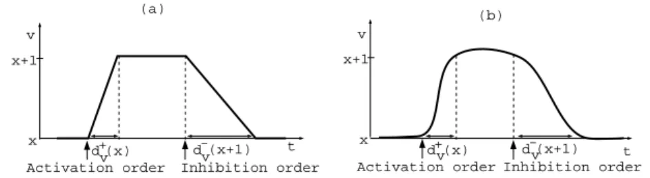
In the semantics that we use, a state can have several successors, each of them corresponding to the evolution of the expression level of a unique gene (the dynamic is asynchronous). One way to overcome this indeterminism is to use timing constraints in terms of parameters with a path algorithm (section 5). These parameters represent time delays for the discrete changes in expression levels of a gene. To be more precise, when an order of activation/inhibition arrives, the biological machinery starts to increase/decrease the corresponding protein concentration, but this action takes time. These times are abstracted by these time delays. We use two types of time delays d+
v(x) and d−v(x) to represent
the time required to change the expression level of a gene v from an abstract level x to x + 1 and from the level x to x − 1 respectively as shown in figure 1.
v t d v + d v
-Activation order Inhibition order (x) (x+1) x+1 x v t dv+ dv
-Activation order Inhibition order (x) (x+1) x
(a) (b)
x+1
Fig. 1. Approximate evolution (a) of the actual evolution (b) of a gene’s expression
4
Example of a BRN
Consider three genes a, b and c which interact according to the graph of figure 2-(a). From this BRN, we obtain the table of resources (figure 2-(c)) and state graph as shown in figure 2-(b).
In the table of figure 2, ωvis the set of resources of a gene v ∈ {a, b, c}, that is
the set of biological entities which helps variable v to increase. The evolution of the expression level of a gene v depends on its resources ωv. Table of figure 2-(c)
helps the reader to reconstruct the state graph representing the dynamics of the BRN. The edges in the graph give the possible transitions between states which can occur with time. The circuit (010, 011, 001, 101, 100, 110, 010) represents an unstable circuit in the dynamics and the two states not involved in the circuit are the only two stable states.
We associate a clock hv, to each variable v ∈ {a, b, c}. All the clocks of the
system increase continuously and simultaneously1. The guard hv == dαv, where
1
It is possible to go from x to x0via the increasing (resp. decreading) of variable v if the time delay d+v (resp. d
−
+ + + a b c (a) 000 100 010 110 011 001 101 111 (b) (C) a b c ωa ωb ωc Ka(ωa) Kb(ωb) Kc(ωc) µ00 0 0 {} {} {} 0 0 0 µ10 0 1 {c} {} {} 1 0 0 µ20 1 0 {} {} {b} 0 0 1 µ30 1 1 {c} {} {b} 1 0 1 µ41 0 0 {} {a} {} 0 1 0 µ51 0 1 {c} {a} {} 1 1 0 µ61 1 0 {} {a} {b} 0 1 1 µ71 1 1 {c} {a} {b} 1 1 1
Fig. 2. BRN (a) and its state graph (b) according to the attractor parameters: Ka({}) = Kb({}) = Kc({}) = 0 and Ka({c}) = Kb({a}) = Kc({b}) = 1.(c)
Asso-ciated table of resources
α ∈ {+, −} gives the condition for the transition. The clock of a variable is set to zero when this variable changes its abstract level. In figure 3 all the transitions are labeled with guards and clock initializations.
011 111 001 101 010 110 000 100 h == d a +a h a 0 h == d c c+ h 0c h == d a -a h 0a h == d b +b h 0b h == d b -b h 0b h == d a +a h 0a h == d c c+ h 0c h == d c c -h 0c h == d b +b h 0b h == d a -a h 0a h == d c c -h 0c h == d b -b h 0b
Fig. 3. Transition system for the BRN of figure 2 along with guard conditions
5
Searching paths between two states
The analysis of the hybrid refinement of the BRN is performed by using a linear hybrid model checker HyTech [HHWT97]. The delays are defined as parameters whose values are unknown. We associate timing constraints with qualitative states of a BRN in terms of time delay parameters. Our path algorithm finds all the possible paths between two qualitative states of a regulatory network. We have implemented this algorithm in HyTech and obtained the exact path between any two qualitative states of a BRN by applying timing constraints in terms of delay parameters.
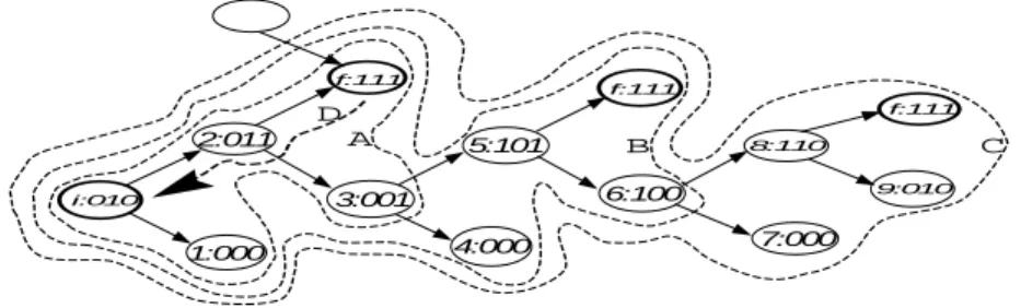
Algorithm 1 is the pseudocode of the HyTech implementation. pre and post operators returns respectively the predecessors and successors of a state includ-ing the state itself. The difficulty of the algorithm lies in the fact that it con-verts the breadth-first search (induced by the post operator) into the depth-first search of a path. The algorithm consists of two main loops. In the outer loop the algorithm exhaustively searches the final state from the initial state and accumulates the accessed states in a set named states accumulated. When the algorithm finds the final state then it starts the nested loop and be-gins backward search from final state and takes the intersection of each ac-cessed states with the set states accumulated. If the intersection is not empty then the algorithm gives the intersection as a state of the path which is ac-cumulated in a set path states. Finally the algorithm invokes the procedure print path(path states) to print the states of a path in proper order.
i:010 f:111 1:000 3:001 2:011 4:000 5:101 6:100 7:000 A B C D f:111 f:111 8:110 9:010
Fig. 4. How the algorithm finds the final states from initial state and vice versa. The empty state shows the accessibility of final state through other path
The dashed lines (A), (B) and (C) of figure 4 represent the successive sets of accumulated states when the algorithm finds the final state f during the outer loop. The inner loop is used for backward search and the dashed arrow (D) shows this search for the first path. Algorithm 1 finds the three paths between states (0,1,0) and (1,1,1) in the example of figure 3.
6
Parameters synthesis
The delay parameters used for the increasing and decreasing of the expression level of a gene v can be synthesized in HyTech to form timing constraints for each transition that takes place in paths between two states. The conjunction of constraints along any sequence of transitions gives the synthesized parameters constraint for the given path.
– For the transition (0,1,0) → (0,1,1): d+ c ≤ d
− b
– For the transition (0,1,1) → (0,0,1): d−b ≤ d+ a
– For the transition (0,0,1) → (1,0,1): d+
c + d+a ≤ d−a + d − b + d
− c
– For the transition (1,0,1) → (1,1,1): d+ a + d + b ≤ d − c ∧ d+a + d+c ≤ d−a + d − b
Algorithm 1Finds paths between two states 1:Path(initial state, final state)
2:states accessed :=initial state; // The first accessed states is the initial state 3:reached := initial state; // The first visited state is the initial state 4:path := initial state; // Path is set to initial state
5:states accumulated := initial state;
6:// while exist accessible states of a BRN from initial state 7:while not empty(states accessed) do
8: // The set of accessed states is now the successors of the previously accessed states 9: states accessed := post(states accessed) - states accessed;
10: path := states accessed - path; // Find new states of a path
11: states accumulated := states accumulatedS path; // Set that accumulates the states 12: states accumulated := states accumulated - initial state; // Remove the initial state from
the set
13: states accessed := states accessed - reached; // Remove all previously visited states from set of accessed states
14: reached :=reachedS states accessed; // The previously visited states will now be the accessed states
15: // Check if final state is accessed 16: if not empty(pathT final state) then 17: states accessed1:= final state; 18: reached1 := final state; 19: path1:=final state;
20: //The nested loop starts here 21: while not empty(states accessed1) do
22: // The set of accessed states is now the predecessors of the previously 23: // accessed states in a set of accumulated states
24: states accessed1 := (pre(states accessed1)-states accessed1)T states accumulated; 25: path1:=states accessed1 - path1;
26: path states := path statesS path1; // Set that accumulates the states of one discovered path
27: states accessed1 := states accessed1 - reached1; 28: reached1:= reached1S states accessed1; 29: end while
30: print path(path states); // To print the states of a path 31: end if
32: end while
Now if we desire to find only the path shown by the bold line in figure 3, then we use the timing constraints which are synthesized2 by HyTech for the
transitions in one path starting from a state where ha = hb = hc = 0 (see
below). Thus, we draw an equivalence between the path (0, 1, 0) → (0, 1, 1) → (0, 0, 1) → (1, 0, 1) → (1, 1, 1) and the region described by the conjunction of constraints: (d+ c ≤ d − b) ∧ (d − b ≤ d+a) ∧ (d+c + d+a ≤ d−a + d − b + d−c) ∧ (d+a + d + b ≤ d−c) ∧ (d+a + d+c ≤ d− a + d − b).
7
Conclusion
We propose in this paper a refinement based on delays for BRN modelling. The introduction of delays allows one to distinguish paths from one state to another one. This refinement reintroduces time in the abstraction of R. Thomas, and this way is different from the refinement of [BRdJ+05] and [AS04] which split
the state space by partitioning the domains of the state space. The present work describes how the introduction of time can be helpful for modeling such
2
networks, allowing the modeller to verify temporal properties. It is now crucial to confront this modelling with real experiments. Our experience in modeling in a multidisciplinary context will help to initiate biological modeling with delays. Our future work is threefold: (1) formal representation of parameters con-straints, (2) parameter synthesis: we have to check when a path is equivalent to an empty region and what this really means, and (3) cycles: we have to check if there are cycles in the state graph of a BRN.
References
[AS04] M. Ad´ela¨ıde and G. Sutre. Parametric analysis and abstraction of genetic regulatory networks. In Proc. 2nd Workshop on Concurrent Models in Molecular Biology (BioCONCUR’04), London, UK, Aug. 2004, Electronic Notes in Theor. Comp. Sci. Elsevier, 2004.
[BCRG04] G. Bernot, J.-P. Comet, A. Richard, and J. Guespin. Application of for-mal methods to biological regulatory networks: Extending Thomas’ asyn-chronous logical approach with temporal logic. Journal of Theoretical Bi-ology, 229(3):339–347, 2004.
[BRdJ+05] G. Batt, D. Ropers, H. de Jong, J. Geiselmann, M. Page, and D. Schneider.
Qualitative analysis and verification of hybrid models of genetic regulatory networks: Nutritional stress response in Escherichia coli. In M. Morari and L. Thiele, editors, Eighth International Workshop on Hybrid Systems: Computation and Control, HSCC 2005, volume 3414 of Lecture Notes in Computer Science, pages 134–150. Springer, 2005.
[DHL03] V. Devloo, P. Hansen, and M. Labb´e. Identification of all steady states in large networks by logical analysis. Bull. Math. Biol., 65(6):1025–51, 2003. [dJ02] H. de Jong. Modeling and simulation of genetic regulatory systems: a
literature review. J. Comput. Biol., 9(1):67–103., 2002.
[dJGB+04] H. de Jong, J. Geiselmann, G. Batt, C. Hernandez, and M. Page. Qualita-tive simulation of the initiation of sporulation in Bacillus subtilis. Bulletin of Mathematical Biology, 66(2):261–299, 2004.
[dJGHP03] H. de Jong, J. Geiselmann, C. Hernandez, and M. Page. Genetic network analyzer: qualitative simulation of genetic regulatory networks. Bioinfor-matics, 19(3):336–44., 2003.
[HHWT97] T-A. Henzinger, P-H. Ho, and H. Wong-Toi. HYTECH: A model checker for hybrid systems. International Journal on Software Tools for Technology Transfer, 1(1–2):110–122, 1997.
[Sno89] E.H Snoussi. Qualitative dynamics of a piecewise-linear differential equa-tions : a discrete mapping approach. DSS, 4:189–207, 1989.
[ST93] E.H. Snoussi and R. Thomas. Logical identification of all steady states : the concept of feedback loop caracteristic states. Bull. Math. Biol., 55(5):973– 991, 1993.
[Tho78] R. Thomas. Logical analysis of systems comprising feedback loops. J. Theor. Biol., 73(4):631–56, 1978.
[Tho91] R. Thomas. Regulatory networks seen as asynchronous automata : A logical description. J. theor. Biol., 153:1–23, 1991.
[TK01] R. Thomas and M. Kaufman. Multistationarity, the basis of cell differenti-ation and memory. Chaos, 11:180–195, 2001.