OPTIMIZATION OF ALGORITHMS WITH THE OPAL FRAMEWORK
CONG KIEN DANG
D´EPARTEMENT DE MATH´EMATIQUES ET DE G´ENIE INDUSTRIEL ´
ECOLE POLYTECHNIQUE DE MONTR´EAL
TH`ESE PR´ESENT´EE EN VUE DE L’OBTENTION DU DIPL ˆOME DE PHILOSOPHIÆ DOCTOR
(MATH ´EMATIQUES DE L’ING ´ENIEUR) JUIN 2012
c
´
ECOLE POLYTECHNIQUE DE MONTR´EAL
Cette th`ese intitul´ee :
OPTIMIZATION OF ALGORITHMS WITH THE OPAL FRAMEWORK
pr´esent´ee par : DANG Cong Kien
en vue de l’obtention du diplˆome de : Philosophiæ Doctor a ´et´e dˆument accept´ee par le jury d’examen constitu´e de :
M. LE DIGABEL S´ebastien, Ph.D., pr´esident
M. AUDET Charles, Ph.D., membre et directeur de recherche
M. ORBAN Dominique, Doct.Sc., membre et codirecteur de recherche M. BASTIN Fabian, Doct.Sc., membre
Acknowledgements
I am deeply grateful to my supervisors Charles Audet and Dominique Orban. Their academic knowledge, creativity, availability and particularly great efforts to explain things clearly and simply guided me through my exploration and helped shape my work in many important ways.
I would like to show my gratitude to my friends, Thu Lan and Phuong Anh, who helped me greatly during the writing process of my thesis. Not only did I take advantage of their detailed corrections but I also learned a lot to improve my writing skills.
Many thanks to everyone in GERAD, in the department of Applied Mathematics and Industrial Engineering, as well as in Center of Consultation in Mathematics who have helped me out in one way or another. A new life, new working environments, new culture gave me a lot of difficulties, without help and understanding, I could not have this final happy ending.
Finally, I would like to thank my parents, my wife and my sister of their continuous, infinite supports.
R´
esum´
e
La question d’identifier de bons param`etres a ´et´e ´etudi´ee depuis longtemps et on peut compter un grand nombre de recherches qui se concentrent sur ce sujet. Certaines de ces recherches manquent de g´en´eralit´e et surtout de re-utilisabilit´e. Une premi`ere raison est que ces projets visent des syst`emes sp´ecifiques. En plus, la plupart de ces projets ne se concentrent pas sur les questions fondamentales de l’identification de bons param`etres. Et enfin, il n’y avait pas un outil puissant capable de surmonter des difficult´e dans ce domaine. En cons´equence, malgr´e un grand nombre de projets, les utilisateurs n’ont pas trop de possibilit´e `a appliquer les r´esultats ant´erieurs `a leurs probl`emes.
Cette th`ese propose le cadre OPAL pour identifier de bons param`etres algorith-miques avec des ´el´ements essentiels, indispensables. Les ´etapes de l’´elaboration du cadre de travail ainsi que les r´esultats principaux sont pr´esent´es dans trois articles correspondant aux trois chapitres 4, 5 et 6 de la th`ese.
Le premier article introduit le cadre par l’interm´ediaire d’exemples fondamentaux. En outre, dans ce cadre, la question d’identifier de bons param`etres est mod´elis´ee comme un probl`eme d’optimisation non-lisse qui est ensuite r´esolu par un algorithme de recherche directe sur treillis adaptatifs. Cela r´eduit l’effort des utilisateurs pour accomplir la tˆache d’identifier de bons param`etres.
Le deuxi`eme article d´ecrit une extension visant `a am´eliorer la performance du cadre OPAL. L’utilisation efficace de ressources informatiques dans ce cadre se fait par l’´etude de plusieurs strat´egies d’utilisation du parall´elisme et par l’interm´ediaire d’une fonctionnalit´e particuli`ere appel´ee l’interruption des tˆaches inutiles.
Le troisi`eme article est une description compl`ete du cadre et de son impl´ementation en Python. En plus de rappeler les caract´eristiques principales pr´esent´ees dans des travaux ant´erieurs, l’int´egration est pr´esent´ee comme une nouvelle fonctionnalit´e par une d´emonstration de la coop´eration avec un outil de classification. Plus pr´ecis´ement, le travail illustre une coop´eration de OPAL et un outil de classification pour r´esoudre un probl`eme d’optimisation des param`etres dont l’ensemble de probl`emes tests est trop grand et une seule ´evaluation peut prendre une journ´ee.
Abstract
The task of parameter tuning question has been around for a long time, spread over most domains and there have been many attempts to address it. Research on this question often lacks in generality and re-utilisability. A first reason is that these projects aim at specific systems. Moreover, some approaches do not concentrate on the fundamental questions of parameter tuning. And finally, there was not a powerful tool that is able to take over the difficulties in this domain. As a result, the number of projects continues to grow, while users are not able to apply the previous achievements to their own problem.
The present work systematically approaches parameter tuning by figuring out the fundamental issues and identifying the basic elements for a general system. This provides the base for developing a general and flexible framework called OPAL, which stands for OPtimization of ALgorithms. The milestones in developing the framework as well as the main achievements are presented through three papers corresponding to the three chapters 4, 5 and 6 of this thesis.
The first paper introduces the framework by describing the crucial basic elements through some very simple examples. To this end, the paper considers three ques-tions in constructing an automated parameter tuning framework. By answering these questions, we propose OPAL, consisting of indispensable components of a parameter tuning framework. OPAL models the parameter tuning task as a blackbox optimiza-tion problem. This reduces the effort of users in launching a tuning session.
The second paper shows one of the opportunities to extend the framework. To take advantage of the situations where multiple processors are available, we study various ways of embedding parallelism and develop a feature called ”interruption of unnecessary tasks” in order to improve performance of the framework.
The third paper is a full description of the framework and a release of its Python implementation. In addition to the confirmations on the methodology and the main features presented in previous works, the integrability is introduced as a new feature of this release through an example of the cooperation with a classification tool. More specifically, the work illustrates a cooperation of OPAL and a classification tool to solve a parameter optimization problem of which the test problem set is too large and
Table of Contents
Acknowledgements . . . iii
R´esum´e . . . iv
Abstract . . . v
Table of Contents . . . vii
List of Tables . . . x
List of Figures . . . xi
List of Appendices . . . xii
Acronyms and abbreviations . . . xiii
Chapter 1 INTRODUCTION . . . 1
Chapter 2 EMPIRICAL OPTIMIZATION OF ALGORITHMS: STATE OF THE ART . . . 5
2.1 Automatic parameter tuning is an active research area . . . 5
2.2 The basic questions of an automated tuning method . . . 11
2.2.1 Parameterizing the target algorithm . . . 12
2.2.2 Empirical quality evaluation methods . . . 13
2.2.3 Search methods for exploring parameter space . . . 15
2.3 Automatic parameter tuning as an optimization problem . . . 17
2.3.1 Formulation of a parameter optimization problem . . . 17
2.3.2 Direct-search methods for solving blackbox optimization problem 18 2.3.3 The MADS algorithm and the NOMAD solver . . . 22
Chapter 4 Article 1: ALGORITHMIC PARAMETER OPTIMIZATION OF
THE DFO METHOD WITH THE OPAL FRAMEWORK . . . 29
4.1 Introduction . . . 30
4.2 Optimization of Algorithmic Parameters . . . 33
4.2.1 Black Box Construction . . . 34
4.2.2 Direct Search Algorithms . . . 36
4.3 The OPAL Package . . . 37
4.3.1 The OPAL Structure . . . 38
4.3.2 Usage of OPAL . . . 38
4.4 Application to Derivative-Free Optimization . . . 40
4.4.1 General Description of DFO . . . 40
4.4.2 Two DFO Parameter Optimization Problems . . . 41
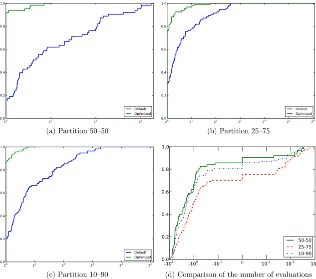
4.4.3 Numerical Results . . . 46
4.5 Discussion . . . 51
Chapter 5 Article 2: EFFICIENT USE OF PARALLELISM IN ALGORITH-MIC PARAMETER OPTIMIZATION APPLICATIONS . . . 52
5.1 Introduction . . . 53
5.2 The Opal framework . . . . 54
5.2.1 Parameter optimization as a blackbox optimization problem . 55 5.2.2 Computational cost reduction with Opal . . . . 55
5.3 Parallelism in algorithmic parameter optimization . . . 56
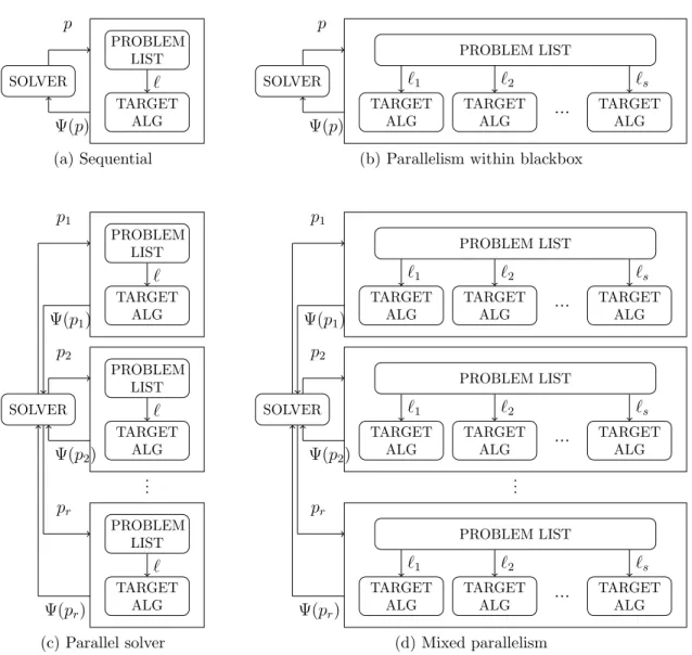
5.3.1 The blackbox solver handles the parallelism . . . 56
5.3.2 Parallelism within the blackbox . . . 58
5.3.3 Mixed parallelism . . . 59
5.4 Numerical results . . . 60
5.4.1 The target algorithm: A trust-region method for unconstrained optimization . . . 60
5.4.2 The parameter optimization problem . . . 61
5.4.3 Comparative study of parallelism within Opal . . . . 62
5.5 Outlook . . . 67
Chapter 6 Article 3: OPTIMIZATION OF ALGORITHMS WITH OPAL . 69 6.1 Introduction . . . 69
6.2.1 Algorithmic Parameters . . . 71
6.2.2 A Blackbox to Evaluate the Performance of Given Parameters 73 6.2.3 Blackbox Optimization by Direct Search . . . 74
6.3 The OPAL Package . . . 77
6.3.1 The Python Environment . . . 77
6.3.2 Interacting with Opal . . . . 80
6.3.3 Surrogate Optimization Problems . . . 82
6.3.4 Categorical Variables . . . 84
6.3.5 Parallelism at Different Levels . . . 86
6.3.6 Combining Opal with Clustering Tools . . . . 87
6.3.7 The Blackbox Optimization Solver . . . 87
6.4 Discussion . . . 88
Chapter 7 GENERAL DISCUSSION . . . 90
Chapter 8 CONCLUSION AND RECOMMENDATIONS . . . 92
Bibliography . . . 95
Appendix . . . 104
A.1 Direct Optimization of some IPOPT Parameters . . . 106
List of Tables
4.1 Algorithmic Parameters of DFO. . . 41
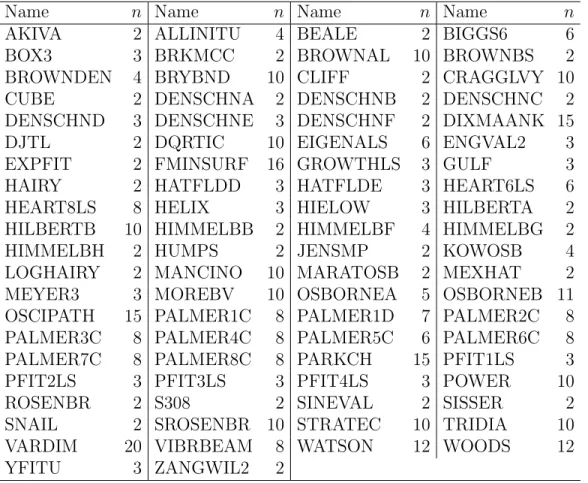
4.2 Unconstrained problems from the CUTEr collection . . . 42
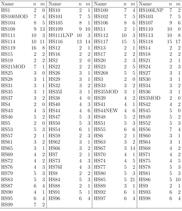
4.3 Constrained problems from the Hock-Schittkowski collection . 44 4.4 Optimized Parameters for different parameter optimization prob-lems and different test problem sets . . . 46
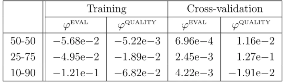
4.5 Cross-Validation Results on Unconstrained Test Problems . . 47
4.6 Cross-Validation Results on Constrained Test Problems . . . . 47
5.1 Test set. . . 63
5.2 Solutions produced from the initial point p0 . . . 64
5.3 Solutions produced from the initial point pcpu . . . 64
A.1 Six IPOPT parameters . . . 105
List of Figures
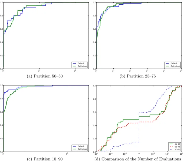
2.1 Classification of direct-search methods . . . 19 2.2 Meshes and poll sets with different sizes . . . 23 4.1 Schematic Algorithmic Parameter Optimization Framework . 34 4.2 Profiles for (4.3) on Each Cross-Validation Set. . . 49 4.3 Profiles for (4.4) on Each Cross-Validation Set. . . 50 5.1 High level representation of the sequential and parallel
strate-gies in Opal . . . 57 5.2 Objective function value versus wall clock time from the initial
point p0. . . 65
5.3 Objective function value versus wall clock time from the initial point pcpu. . . 66 6.1 Performance in MFlops of a particular implementation of the
matrix-matrix multiply as a function of the loop unrolling factor and the blocking factor. . . 78 A.1 Performance profiles for the sets of parameters p0 and p1 . . . 108
List of Appendices
Acronyms and abbreviations
AEOS Automated Empirical Optimization of Software ATLAS Automatically Tuned Linear Algebra Software BLAS Basic Linear Algebra Subprograms
CUTEr Constrained and Unconstrained Testing Environment, revisited DFO Derivative-Free Optimization
DIRECT DIviding RECTangles
EGO Efficient Global Optimization
FFTW Fastest Fourier Transform in the West
GRASP Greedy Randomized Adaptive Search Procedure GPS Generalized Pattern Search
ILS Iterated Local Search
IPC Inter-Process Communication LAPACK Linear Algebra PACKage LSF Load Sharing Facility MPI Message Passing Interface MADS Mesh Adaptive Direct Search
MDO Multi-disciplinary Design Optimization MFN Minimum Frobenius Norm
MNH Minimal Norm Hessian MMAS Max-Min Ant System
MILP Mixed Integer Linear Programming NOMAD Nonlinear Optimization with MADS OPAL OPtimization of ALgorithms
ORBIT Optimization by Radial Basis function Interpolation in Trust region PHiPAC Portable High Performance Ansi C
RBF Radial Basis Function
SKO Sequential Kriging Optimization SOM Self-Organizing Map
SPO Sequential Parameter Optimization
STOP Selection Tool for Optimization Parameters
TRUNK Trust Region method for UNKonstrained optimization VNS Variable Neighborhood Search
Chapter 1
INTRODUCTION
Despite progresses in computational technology, the need to improve numerical routines remains. We need to improve performance in terms of computational resource consumption and computing time; we wish to achieve better results in precision; or we simply want to extend the applicability of routines in terms of solvable problem classes. In practice, for a numerical routine, it is possible to improve on any of the three phases of its lifetime: design, implementation and operation. In the design and implementation phases, performance is determined by algorithm complexity, local convergence or evaluation complexity (Cartis et al., 2012), while quality is assessed by global convergence or numerical stability (Higham, 2002). In the operation phase, quality and performance are reflected in measurable and less abstract notions such as computing time, memory consumption and accuracy (in terms of significant digits, etc). No matter what forms they take, performance and quality are usually sensitive notions influenced by a large number of factors. In order to control the quality and performance of a routine, we try to capture as many influencing factors as possible, model them as parameters and assign suitable values. Any modification in the first phase can lead to modifications in the next two phases and normally results in a new algorithm or routine. Modifications in the implementation phase that aim at better performance or quality are referred to as source code adaptation. Choosing a suitable setting for parameters at run time is called parameter tuning. Parameter tuning can be done manually using trial and error or automatically by a finite procedure. It can also be done analytically by exact computations or empirically based on a finite set of input data called test problems. Among these possibilities, our work concentrates on developing a framework for empirical automated parameter tuning.
An empirical method for automated parameter tuning is an iterative method where each iteration executes at least three steps: propose parameter values, evaluate the algorithm with these values and finally make a decision on stopping or continuing to the next iteration. The initial suggestion for parameter values is normally provided
by users or simply the default values. In subsequent iterations, the tuning method suggests other settings using some strategies and information obtained in previous iterations. The strategy is different for each method and becomes one of the charac-teristics that distinguish tuning methods. The evaluation is performed by launching the target routine over a set of preselected test problems. Issues for a quality assess-ment strategy include test problem selection, analyzing the results and quantifying the tuning goals. In the last step, the main task is to compare the obtained quality assessment of the current parameter setting with the tuning goal in order to decide whether to go on to the next iteration or not. There is no standard response to this question and its answer usually depends on users goals. Thus, in combining possi-bilities for each step, there are many ways to build an empirical automated tuning procedure. Parameter tuning is still a research question, which means that there is currently no unique satisfactory method for all users. The difficulty comes from many sources. First of all, it is not easy to identify parameters that impact the tuning ob-jective. The hidden relation between parameters and performance adds uncertainty to any automated tuning strategy. Secondly, the numerous parameters and their dis-tribution create an intricate search space that prevents manual tuning. For example, the routine IPOPT (W¨achter and Biegler, 2006), an interior point solver, has nearly 50 parameters, most of which can be real number. Thus, enumeration of all possibil-ities is impossible and the trial and error strategy is usually unsatisfactory. Finally, an effective tuning strategy usually requires expert knowledge of the algorithm and a thorough understanding of the effects of the parameters. As a consequence, it is not easy to create a general framework that works well on all algorithms.
Recent achievements in optimization, particularly in blackbox optimization, pro-vide another approach to the tuning problem. The tuning question can easily be modeled as an optimization problem, in which variables are the tuning parameters and performance or quality are expressed as objective functions and constraints. As a result, several methods of optimization can be applied here. However, classical opti-mization methods depend strongly on the structure of the problem. With a parameter optimization problem, we do not have much information about the structure except the function value at some given parameter points (each parameter point corresponds to a set of parameter values). The situation becomes even worse when the function value is estimated using uncertain empirical outputs such as computing time. An optimization method that depends less on problem structure and handles the lack
of information on problem structure such as direct-search methods holds promising prospects for solving the parameter optimization problem. We chose MADS (Audet and Dennis, Jr., 2006)(Mesh Adaptive Direct Search) as our fundamental algorithm to solve the parameter optimization problems.
By studying the parameter tuning problem both from the perspective of an iter-ative method and as an optimization problem, we design a framework of algorithmic parameter optimization called OPAL (OPtimization of ALgorithms). OPAL is general and flexible enough to apply to the question of improving the performance of any rou-tine. We concentrate on algorithmic parameters, and thus sometimes we refer to the problem of algorithmic parameter optimization as algorithm optimization. Like many empirical methods, each iteration of our method goes through three steps involving the NOMAD (Le Digabel, 2011), an implementation of the MADS method: (i) NO-MAD proposes a parameter settings, (ii) the target algorithm with these settings is evaluated on a set of test problems, (iii) the evaluation result provides information to NOMAD to launch the next iteration. As a result, we require minimum effort from users to define a parameter optimization problem with the following main elements: parameter description, a set of test problems, evaluation measurements, and tuning goals expressed as an objective function and constraints. After defining a parameter optimization problem, all the remaining work is performed by the NOMAD solver.
In simple situations, users do not need to know and provide much information to launch a parameter tuning session. However, to make the framework more flexible and sophisticated in situations where the users know more about their algorithms, they can provide more information to accelerate the search or guide it toward promising regions. For example, users can refine the parameter space by defining more parameter constraints to prevent unnecessary target algorithm runnings. Users can also define surrogate models for their problems to help NOMAD to propose promising parameter values. In the meantime, from the computing point of view, the tuning process is composed of fairly independent steps, for example, the observation of the algorithm over a set of test problems; thus, there are possibilities to exploit parallelism in the framework.
In this introduction, we have presented a brief overview of the typical research involving algorithmic parameter optimization. In chapter two, we discuss relevant literature with a focus on the three main questions of an empirical method and issues relating to parameter optimization problem. The third chapter gives an outline of
the remainder of the thesis, with chapter 4, 5 and 6 reserved for three papers on this problem. Finally, the last chapter shows some conclusions and perspectives.
Chapter 2
EMPIRICAL OPTIMIZATION
OF ALGORITHMS: STATE OF
THE ART
As presented in the previous chapter, we can improve the performance of a numer-ical routine in the development stage (also known as source code adaptation) and in the operaton stage (also known as parameter tuning). Since source code adaptation can also be considered as parameter tuning of a particular source code generator, hereafter, we use the term parameter tuning to indicate both source code adapta-tion and parameter tuning. In this secadapta-tion, we first review some typical projects involving parameter tuning to show that this is a domain of active research. Next, by identifying common elements of these approaches, we examine how these projects answer three basic questions of an automated parameter tuning procedure: (i) what are the parameters, (ii) how to assess the effect of parameter settings and (iii) how to explore the parameter setting space. In the final section we describe related issues where parameter tuning is examined as a blackbox optimization problem, especially in the context of direct search methods.
2.1
Automatic parameter tuning is an active
re-search area
Better performance can be achieved at the development or operation stage. In the development stage, the binary code generation is optimized in terms of the per-formance that depends on the compiler and the platform where the software is built. There are two approaches for optimizing code generation. The first approach creat-ing an important branch of research, called compiler, is based on analytical studies that are therefore outside of the scope of this thesis. The second one is concerned
with adapting code to the running platform and is based mainly on the combina-tion of empirical studies and search strategies. The search is performed on the set of code transformations allowed at the programming language level and is based on performance evaluation through empirical output.
PHiPAC1(Portable High Performance Ansi C) (Bilmes et al., 1998) is one of the earliest automatic tuning projects that aims to create high-performance linear algebra libraries in ANSI C. It is referred to as a methodology that contains a set of guidelines for producing high-performance ANSI code. It also includes a parameterized code gen-erator based on the guidelines and scripts that automatically tune code for a particular system by varying the generators’ parameters based on empirical results. PHiPAC is used to generate a matrix-matrix multiplier that can get around 90% of peak (on sys-tems such as Sparcstation-20/61, IBM RS/6000-590, HP 712/80i) and on IBM, HP, SGI R4k, Sun Ultra-170, it can even produced a matrix multiplier that faster than the ones of vendor-optimized BLAS2 (Basic Linear Algebra Subprograms) (Lawson
et al., 1979).
ATLAS3(Automatically Tuned Linear Algebra Software) (Whaley et al., 2001), a more recent project on numerical linear algebra routines, is an implementation of the Automated Empirical Optimization of Software paradigm, abbreviated as AEOS. The initial goal of ATLAS was to provide an efficient implementation of the BLAS library. However, ATLAS was recently extended to include higher level routines from the LAPACK (Linear Algebra PACKage) library. ATLAS supports automated tuning in all three levels of BLAS. For level 1 BLAS, which contains routines doing vector-vector operations, ATLAS provides a set of pre-defined codes contributed from many sources (with varying floating point unit usage and loop unrolling) from which a best code is selected based on evaluations of this set. The set of pre-defined code is enriched over time. In fact, tuning by ATLAS at this level does not achieve significant improvements; speedup typically ranges from 0% to 15%. The observed efficiency in level 2 BLAS is much better; the speedup can reach up to 300% in some cases. The reason is that level 2 includes vector-matrix routines that are much more complex than the level 1 routines in terms of both data transfer and loop structure; consequent to these facts, there are more possibilities to be optimized. ATLAS also initiates the
1. http://www.icsi.berkeley.edu/~bilmes/phipac/ 2. http://www.netlib.org/blas/
idea of optimizing BLAS by replacing the global search engine with a model-driven optimization engine based on a robust framework of micro-benchmarking called X-Ray (Yotov, 2006).
The work of Yotov (2006) is not about an empirical method but the contribution to the field is remarkable. It initially starts out to study the differences in the per-formance of BLAS tuned by ATLAS and that supported by compiler restructuring. They firstly study whether there is a compiler restructuring that produces the same code generated by ATLAS. Furthermore, by recognizing the fact that ATLAS uses a fairly simple search procedure to get optimal parameters of the source code genera-tor, the author proposes a model to get these values instead of an iterative method. The model computes optimal values from a set of hardware specifications (such as CPU frequency, instruction latency, instruction throughput, etc) that are gathered by a micro-benchmark system. The experimental results state that a micro-benchmark system of high accuracy with a good model can give as good parameters as those found by ATLAS. This implies that the optimality found by the ATLAS algorithm is proved at certain levels. In order to improve the result, a local search heuristic is applied to a neighborhood of the parameter values computed by the model.
Sparsity4 (Im and Yelick, 1998) and OSKI5 (Optimized Sparse Kernel Interface,
Vuduc et al. 2005) focus on a narrower direction in tuning linear algebra libraries - sparse matrix manipulation. Sparsity addresses the issue of poor performance of general sparse matrix-vector multipliers due to spatial locality. Recognizing that performance is also highly dependent on methods of sparse matrix representation and on hardware platforms, Sparsity allows users to automatically build sparse matrix kernels that are tuned to their target matrices and machines. OSKI, inspired by Sparsity and PHiPAC, is a collection of low-level C primitives for use in a solver or in an application. In OSKI, “tuning” refers to the process of selecting the data structure and code transformations to get the fastest implementation of a kernel in the context of matrix and target machine. The selection is essentially the output of a decision making system whose input are benchmark data of a code transformation, matrix characteristics, workload from program monitoring, history and heuristic models.
In addition to linear algebra libraries, signal processing is a promising ground for 4. http://www.cs.berkeley.edu/~yelick/sparsity/
empirical source code adaptation. Among many projects, SPIRAL6 (P¨uschel et al.,
2005, 2011) is the best example despite its restricted consideration on linear signal transforms. SPIRAL optimizes code by exploiting not only hardware factors but also mathematical factors of transforms (Milder, 2010); it optimizes at both the algorith-mic and the implementation levels. More specifically, a transform can be represented as formulas based on different mathematical factors. Hence, there are usually many choices of representing a single transform. These formulas are next implemented by considering appropriate target programming languages, compiler options, as well as target hardware characteristics. To search for the best combination of representation and implementation, SPIRAL takes advantage of both search and learning techniques. For example, the current version of SPIRAL deploys two search methods: dynamic programming and evolutionary search. The learning is accomplished by reformulat-ing the problem of parameter tunreformulat-ing in the form of a Markov decision process and reinforcement learning. SPIRAL shows very interesting experimental results (P¨uschel et al., 2005), including performance spread with respect to runtime within the for-mula space for a given transform, comparison against the best available libraries, benchmark of generated code for DCT (Discrete Cosine Transformation) and WHT (Walsh-Hadamard Transform) transforms. In summary, the idea behind SPIRAL is to choose the best implementation when we have multiple implementations of multiple formulas of a transform; this is similar to the PetaBricks7 (Ansel et al., 2011) project
that targets scientific softwares.
FFTW8 (Fastest Fourier Transform in the West) (Frigo and Johnson, 2005) is a
C subroutine library for computing the discrete Fourier transform (DFT) in one or more dimensions, of a real or complex input of arbitrary size. The library is able to adapt to a new situation not only in terms of input data size but also performance. The optimization in FFTW is interpreted in the sense that FFTW does not use a fixed algorithm for computing the transform, but instead adapts the DFT algorithm by choosing different plans that work well on underlying hardware in order to in-crease performance. The performance adaptation can be performed automatically by a FFTW component called a planner or manually by advanced users who can customize FFTW. Hence, FFTW is a parameter tuning tool rather than source code
6. http://spiral.net/index.html
7. http://projects.csail.mit.edu/petabricks/ 8. http://www.fftw.org/
adaptation like SPIRAL.
PetaBricks (Ansel et al., 2011) and Orio9 (Hartono et al., 2009) both target the
source code adaptation problem for a program or a segment code in any domain. The generalization is obtained by proposing particular programming directives or even a programming language to specify the possibilities of tuning in the target segment code. PetaBricks allows to tune a target routine in two levels by having multiple implementations of multiple algorithms for a target routine. For example, in order to sort an integer array, we can from several sorting algorithms; and corresponding to the selected algorithm, several implementations are considered. Orio only focuses on the implementation level by proposing an annotation language that is actually the programming directives. A high-level segment code, enclosed by these directives, will be implemented in different ways corresponding to variations of the architecture specifications such as the blocking size, cache size, etc. A good implementation is selected based on the performance of running the generated code.
The work of Balaprakash et al. (2011b) can be considered as a source code adap-tation project in the sense that it formulates with the help of the Orio annoadap-tations the tuning questions of a set of basic kernels used broadly and intensively in scientific applications. These problems are solved for each hardware architecture to obtain the most suitable implementation for each kernel. The contributions to the auto-mated tuning field are the formulas of kernel optimization problems plus a particular algorithm to solve effectively these problems.
In practice, the question of parameter tuning has been studied by many re-searchers. We can list here some examples: optimization of control parameters for genetic algorithms (Grefenstette, 1986), automatic tuning of inlining heuristics (Cava-zos and O’Boyle, 2005), tuning performance of the MMAS (Max-Min Ant System) heuristic (Ridge and Kudenko, 2007), automatic tuning of a CPLEX solver for MILP (Mixed Integer Linear Programming) (Baz et al., 2009), automatic tuning of GRASP (Greedy Randomized Adaptive Search Procedure) with path re-linking (Festa et al., 2010), using entropy for parameter analysis of evolutionary algorithms (Smit and Eiben, 2010), modern continuous optimization algorithms for tuning real and integer algorithm parameters (Yuan et al., 2010). However, all these projects target specific algorithms, maximally take advantage of particular expert knowledge to get the best possible results and avoid the complexity of a general automated tuning framework.
The number of tuning projects continues to increase, indicating that the concern still exists. Thereby, it begs the question of a general framework where the basic questions of automated tuning are imposed and answered more clearly. The recent projects presented in the following paragraphs pay more attention to these questions. STOP10(Selection Tool for Optimization Parameters, Baz et al. 2007) is a tun-ing tool based on software testtun-ing and machine learntun-ing. More specifically, it uses an intelligent sampling of parameter points in the search space assuming that each parameter has a small discrete set of values. This assumption is acceptable for the intended target problem of tuning MILP branch-and-cut algorithms. At the time of re-lease, STOP set the parameter values in order to minimize the total solving time over a set of test problems. No statistical technique is used because the authors assume that good settings on the test problems will be good for other, similar problems.
ParamILS11is a versatile tool for parameter optimization and can be applied to an
arbitrary algorithm regardless of the tuning scenario and objective and with no lim-itation on the number of parameters. It is derived from efforts of designing effective algorithms for hard problems (Hutter et al., 2007). Essentially, it is based on the ILS (Iterated Local Search) (Louren¸co et al., 2010) meta-heuristic. ParamILS is supported by a verification technique that helps to avoid over-confidence and over-tuning. How-ever, due to the characteristics of the employed local search algorithm, it works only with discrete parameters; continuous parameters need to first be discretized. More-over, local search performance depends strongly on neighborhood definition that is drawn from knowledge on the parameters of the target algorithm. But ParamILS has not a way to customize the neighborhood definition for a variable.
The above projects are based on heuristics and focus only on specific target algo-rithms or particular parameter types. Recently, the question of parameter tuning was approached more systematically where the connection between the parameter tuning and stochastic optimization is established. These projects are based on a frame-work called Sequential Parameter Optimization (SPO) (Bartz-Beielstein et al., 2010b; Preuss and Bartz-Beielstein, 2007), which is a combination of classical experiment design and stochastic blackbox optimization. The main idea of this approach is to use a stochastic model called a response surface model to predict relations between three principal elements of the automated tuning question: parameters, performance
10. http://www.rosemaryroad.org/brady/software/ 11. http://www.cs.ubc.ca/labs/beta/Projects/ParamILS/
and test problems. Response surface models can be useful in order to study a parame-ter tuning problem in some different aspects: inparame-terpolate empirical performance from evaluated parameter settings, extrapolate to previously-unseen regions of the param-eter space, and qualify the impacts of paramparam-eter settings as well as test problems. SPOT12(Bartz-Beielstein, 2010) is a R package implementing the general idea of SPO that are applied in the context of parameter tuning. Extensions such as SPO+, can be found in the works of Hutter et al. (2010a, 2009).
SPO and our framework OPAL have one thing in common: they both model parameter tuning as a blackbox optimization problem. However, the blackbox model in SPO is assumed to be a stochastic blackbox model while we do not impose any assumption over blackbox model.
2.2
The basic questions of an automated tuning
method
We can identify three common basic elements of all the projects presented in the above section: parameterization, performance evaluation and parameter search strat-egy. The first is the question of identifying variable factors that influence performance and describing these factors in terms of parameters. For algorithmic parameter op-timization, the variables are defined explicitly; thus identifying parameters is usually not difficult. In contrast, identifying variables for source code adaptation is often difficult since source code performance is influenced by many hidden factors. In ad-dition to the parameter identification, it is necessary to define the parameter space by specifying the domain for each parameter, simple relations between parameters.
The second question is about assessing the quality of parameter settings. In other words, it is the problem of comparing the empirical performance of the target algorithm with various parameter settings. Obviously, this question depends on the tuning objective. In general, comparison criteria are established based on observations of running the algorithm over the set of test problems, such as computing time, consumed memory, and/or algorithm output. In the simplest case, we can choose an observation as a criterion of comparison, but criteria can be expressed in more sophisticated ways such as a function and even as an output of a computation process
or a simulation process whose inputs are the observations from running the target algorithm. The main concern for an assessment method is the inaccuracy that comes from two sources: uncertainty of some observations and empirical noise. However, it is not possible to totally eliminate the inaccuracy; we often must balance the cost of inaccuracy reduction and the sophistication of a search method.
The last question concerns the search strategy in parameter space. The complexity of a strategy depends on the two previous questions. The larger the parameter space is, the more sophisticated the strategy we need. The less accurate the performance evaluation is, the more flexible the search strategy we need to come up with. The more specific the application is, the more particular the knowledge is to be integrated into the strategy. The fact of the matter is we have no guide to build a search strategy.
2.2.1
Parameterizing the target algorithm
The process of algorithm parameterization is composed of two tasks: identifying parameters and describing them. The former will imply which parameters are in-volved. Parameters of an algorithm (or a routine) are generally all the factors that can be changed by an user of the algorithm that have an impact on the implementa-tion’s performance. For the code adaptation, these factors vary from one language to another, and from one architecture to another. However, the spectrum of code gener-ators’ parameters is usually not very broad. As a consequence, parameter spaces can be described well once the parameters are identified. In contrast, identifying param-eters in algorithmic parameter tuning is less difficult but describing the parameter space or selecting a subset of parameters which are significant is a big issue.
ATLAS optimizes the BLAS library using both techniques, parameter tuning and source code adaptation. In the former, ATLAS focuses on parameters of the library kernels such as the blocking factor and the cache level. These parameters control the cache utilization and as a consequence, directly influence speedup. The source code adaptation is performed by choosing the best code from a pre-fixed set of codes provided by many contributors or by automatically generating codes from templates. In the first approach, we have a single parameter whose possible values correspond to the set of contributions of source code. In the second approach, the set of parameters of a template includes L1 data cache tile size, the L1 data cache tile size for non-copying version, register tile size, unroll factor, latency for computation scheduling,
choices of combined or separate multiply and add instructions and load scheduling. Corresponding to each combination of parameter settings, a source code of the routine is generated from the template. For other projects concentrating on linear algebra routines (except for Sparsity and OSKI which exploit particularities of sparse matrices), the set of involved parameters is typically selected from the set proposed by ATLAS. Most project have parameters expressing the selections called the selecting pa-rameters. The domain of this parameter type is sometimes simple as an unordered set of values. ATLAS uses a categorical parameter to indicate a the set of predefined code. Sometime, the domain is a set of a particular order such as the case of the plan selecting parameter in FFTW or the component selecting in ParamILS. The domain can be so complicated to be represented by a set, for example, each selection of the algorithm selecting parameter in PetaBrick is represented as a tree.
For some tuning projects that includes a selecting components, the parameter space can be changed corresponding to each selection. For example, SPIRAL opti-mizes a routine by finding the most suitable implementation of a transform. In order to get a possible implementation for a transform, SPIRAL translates the transform to formulas, and codes these formulas in a target programming language. Parameters of the formula generation stage include the atomic size of formula, formula character-istics such as parallelizable construct or vectorizable construct. Hence, in the second stage, in addition to the parameters of a code generator, the particular parameters of the selected formulas will be considered.
2.2.2
Empirical quality evaluation methods
Empirical quality evaluation involves the process of comparing performance of two instances of parameters through a set of experiments, and it is sometimes referred to as experimental comparison. More concretely, within the context of an empirical automated tuning project, the assessment is performed through a sequence of tasks, running the target algorithm over a set of test problems, collecting all concerned ob-servations (referred to as atomic measures in OPAL terminology) on each test problem and building comparison criteria (referred to as composite measures in OPAL termi-nology) from the observations. Examples of observations are wall-clock running time and outputs of the algorithm (such as the solution, number of significant digits of so-lution, norm of the gradient, etc). There are two main issues related to the empirical
comparison. The first is that atomic measures are often noisy. A typical example is the wall-clock time: running the target algorithm on a machine can result in different running times in different launches due to operating system, influence. The second is that, because observations are obtained from running algorithm over a set of test problems, they are concrete instances of a performance measure. A better perfor-mance based on these concrete instances does not guarantee a better perforperfor-mance in general or on other instances. The different techniques of quality evaluation deal with the two issues in different ways.
The simplest way to deal with the noise of some elementary measures is to choose an alternative one that is less noisy. For example, to benchmark an optimization solver, the number of function evaluations may be more suitable than the com-puting time. CUTEr (Constrained and Unconstrained Testing Environment, revis-ited) (Gould et al., 2003a) is a project that provides systematic measures for assessing an optimization solver. To provide a general description of CUTEr13,
it is a versatile testing environment for optimization and linear algebra solvers. The package contains a collection of test problems, along with Fortran 77, Fortran 90/95 and Matlab tools intended to help developers design, compare and improve new and existing solvers.
CUTEr provides a mechanism to extract the number of metrics (such as objective functions and constraint functions, the final value of objective function, of gradient norm, etc). Such a performance assessment of an optimization solver may better reflect the practical performance of a solver, independent of the platform.
Other common ways to address the noise are drawn from statistics. For exam-ple, the noise of an observation can be reduced by repeatedly launching the target algorithm over the set of test problems and taking the sampled mean value. This treatment is expensive in terms of computational resources. A more efficient way is to think of each test problem as a sample drawn from a problem population; and that an analysis over a good enough sample set can achieve accurate descriptions of dependences between performance and the parameters. Answers to the question of how to get an accurate description are summarized in Kleijnen (2010) and result in a methodology called design of experiments. Statistical design of experiments is the process of first planning an experiment so that appropriate data is collected and ana-lyzed using statistical methods so that useful conclusions can be drawn. For example,
CALIBRA (Adenso-Diaz and Laguna, 2006) employs fractional factorial designs to draw conclusions based on a subset of experiments from a set of pk possible
combina-tions of parameters where k is the number of parameters and p is number of critical values of each parameter. The strategy for selecting the subset from the total set is that of Taguchi et al. (2004), which uses orthogonal arrays to lay out the experiments. CALIBRA uses the L9(34) orthogonal array that can handle up to 4 parameters with 3
critical values by just 9 experiments. More examples can be found in Bartz-Beielstein et al. (2010a), a book on experiment design techniques specialized to parameter tun-ing with a particular focus on sequential techniques that instruct how to select new promising points based on information obtained from previous experiments.
Another research area that can be involved in empirical evaluation is the concept of performance and data profiles of Dolan and Mor´e (2002) and Mor´e and Wild (2009) for comparing solvers through a set of test problems. In the context of parameter tuning, the target algorithm associated with each parameter setting is regarded as a solver. These profiles provide a visual qualitative information, and hence a method to get a quantitative output from performance profiles can be a good empirical assessment method, for example, the area of the region below a profile curve.
In addition to techniques of treating measures and observation, selecting a good test problem set can significantly improve the extrapolatory quality of the evaluations. Although the set of test problems is pre-selected, having awareness of the influences of the test problems is necessary for a good empirical result analysis. More detailed arguments can be found in Auger et al. (2009) and Hutter et al. (2010b).
2.2.3
Search methods for exploring parameter space
In any method of empirical quality evaluation, there is an assumed model that expresses the relation between parameter value combinations and observations or quality. The model can be formulated implicitly as a blackbox (Audet and Orban, 2006) or explicitly as a stochastic model (Bartz-Beielstein et al., 2010b) or as a deter-ministic model (Yotov, 2006). Search strategies must take into account the parameter space representation as well as the method of quality assessment.
Most parameter tuning projects choose heuristic approaches. Targeting a specific problem, taking advantage of particular descriptions about the parameters, a heuristic may get good performance. However, the flexibility is often reduced as efficiency is
gained. There are some projects that develop their heuristic from a meta-heuristic; if the development does not involve too much particularities, it can be extended or be modified to deploy in other projects. For example, ParamILS (Hutter et al., 2007) is developed from the ILS (Louren¸co et al., 2010) meta-heuristic, which proposes iterative jumps to other regions after reaching a local optimum of the current region. ILS leaves users free to choose a method to find local minima as well as how to jump to another region. ParamILS approaches parameter tuning with the two most basic ingredients: search a better solution by a simple procedure and as soon as finding it, jump to another region by a random move.
Besides the dependence of performance on particularities, most heuristics work with finite discrete sets, which means that a tuning algorithm based on these heuristics can only work on categorical parameters or integer parameters with bounds. For real parameters, these methods require a discretization without loosing information phase that may be costly. Moreover, heuristics can only handle simple parameter spaces that are composed of a small number of variables and each variable may have few values.
As mentioned previously, an experiment design method includes not only tech-niques for drawing conclusions from experimental results, but also techtech-niques to set up or control experiments. In the context of parameter tuning, the latter techniques will figure out potential parameter settings where the tests can manifest all the char-acteristics of the target algorithm, hence most simply, we can choose one of suggested settings as the solution. There is a class of techniques called the sequences of exper-iments that suggest the next settings to examine based on the result of experexper-iments performed. The SPO search strategy is built based on this theory.
In reality, three basic questions are tightly corded. However, previous projects have focused on each question separately or not paid enough attention to the relations between them. This is one possible reason why the proposed tuning techniques in the literature have remained non-systematic approaches. In the next section, we study the parameter tuning problem from the optimization point of view where the three basic questions are examined in a unique model.
2.3
Automatic parameter tuning as an
optimiza-tion problem
In the optimization community, the automated tuning parameter question may be formulated as an optimization problem where variables are the involved parameters and the tuning objective and the context are expressed by objective function and constraints, respectively. By formulating as a blackbox problem, minimal information on problem structure is required. This means that users can easily and quickly define a parameter optimization problem and rely on the chosen solver. Nonetheless, it does not prevent the possibility of providing more specific information to accelerate the search process.
2.3.1
Formulation of a parameter optimization problem
We formulate the parameter tuning problem as a blackbox optimization problem. The simplest statement of a parameter optimization problem is
minimize
p ψ(p)
subject to p ∈ P ϕ(p) ∈ M
(2.1)
where p denotes a parameter vector; P represents the valid parameters region; the objective function ψ(p) expresses the tuning objective; and general constraints ϕ(p) ∈ M encode the restrictions of the tuning process. Note that the elements of a vector parameter p are not necessary of the same type. An element can be one of three following types: a real number (type R), an integer number (type Z) or a categorical value (type C) (Audet and Dennis, Jr., 2000). Hence, if a target parameter set has n parameters of type R, m parameters of type Z and l categorical parameters, a vector p is an element of Rn× Zm
× Cl. The valid parameter region, P, is a subset of
Rn× Zm× Cl that models the parameter region reacts such as a positive number or a real number in the interval (0, 1). The target algorithm assessment result is expressed in the objective function ψ(p) and the general constraints ϕ(p) ∈ M. The reason why we split the constraints in two categories p ∈ P and ϕ(p) ∈ M is that the former is used to validate a parameter setting and decide if we need to launch the target algorithm over the test problems while the latter is only verified if all runnings are
terminated.
Another attempt to bring automated tuning into the optimization community is proposed by Balaprakash et al. (2011b) where the parameter optimization problem is stated simply as
min
x {f (x) : x = (xB, xI, xC) ∈ D ⊂ R
n} (2.2)
where xB, xI and xCcorrespond to the binary, integer and continuous parameters, and
f (.) is some performance measure. The efficiency of solving 2.2 depends on the domain D whose the construction requires expertise knowledge on the target algorithm. In other words, this formulation does not give much information to a solving method until the domain D is well established.
A blackbox optimization problem can be solved by using a direct-search solver or a heuristic. The heuristic efficiency depends strongly on the expert knowledge. In the general case of a blackbox optimization problem, we assume that there is no information except for function values at certain points; this implies the inefficiency of heuristic methods. Thus, we reserve the next subsection for discussing only direct-search methods.
2.3.2
Direct-search methods for solving blackbox
optimiza-tion problem
Direct-search solvers comprise all methods that use only functions values (objec-tive and constraints) to search for a local optimum. These methods are distinguished from classical methods that require first order-information (derivative, gradient), such as gradient-based methods or even second order-information (Hessian matrix), such as Newton methods. Direct-search methods form only a subset of derivative-free meth-ods that includes methmeth-ods that approximate derivatives or use derivative-like concepts such as sub-gradients (Conn et al., 2009b). Focusing only on methods that work well for blackbox optimization, we review results of direct-search methods. There are two main ideas for direct-search methods. The first one is to use a model to guide iterates approaching a local optimum, the methods are classified as model-based methods. The model can be a local approximation of the objective function and its precision is improved from iteration to iteration. Another option is stochastic models that cap-ture the global characteristics of the functions. The second idea is based on sampling variable domains; at each iteration, the variable domain is sampled at certain points
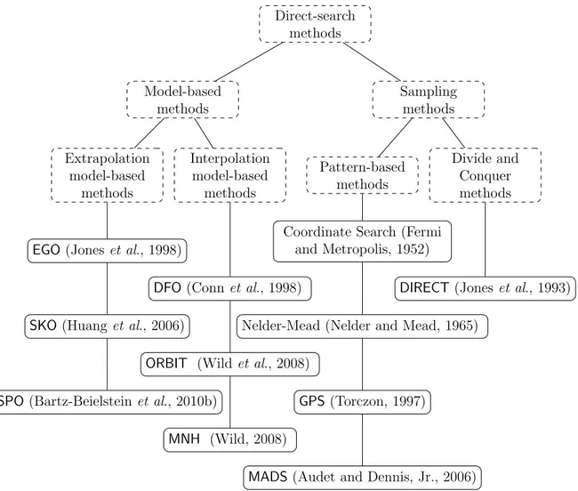
depending on a sampling strategy to evaluate the objective function. This branch is in turn divided into two sub-categories, such divide-and-conquer and pattern-based are sometimes referred to as directional search. Figure 2.1 illustrates some state-of-art methods that are considered as fundamental ideas; variants and derived methods now constitute a rich set of direct-search methods.
Direct-search methods Model-based methods Sampling methods Extrapolation model-based methods Interpolation model-based methods Pattern-based methods Divide and Conquer methods
EGO (Jones et al., 1998)
SKO (Huang et al., 2006)
SPO (Bartz-Beielstein et al., 2010b)
DFO (Conn et al., 1998)
ORBIT (Wild et al., 2008)
MNH (Wild, 2008)
Coordinate Search (Fermi and Metropolis, 1952)
Nelder-Mead (Nelder and Mead, 1965)
GPS (Torczon, 1997)
MADS (Audet and Dennis, Jr., 2006)
DIRECT (Jones et al., 1993)
Figure 2.1 Classification of direct-search methods
The DFO (Derivative-Free Optimization) (Conn et al., 1998) method locally mod-els the objective function by quadratic interpolation and uses this local model to find the next iterate. In each iteration, the local optimum of the model within a trust region is chosen as the next iterate if the reduction of the model and the reduction of the objective/merit function at this point are compatible. Otherwise, the method remains at the incumbent point and tries to find a local minimum of the model in a
smaller region. In both cases, the model is updated in order to improve its quality by adding to the interpolation set a new point satisfying a well-poisedness condition (for example Λ-poisedness, where Λ is a constant related to geometry of the interpolation set). In practice, DFO uses a quadratic model that is not expensive to construct and optimize. The idea behind this procedure is that interpolation models can accurately represent the objective function that can be a smooth (twice differentiable) function over a small region. However, the interpolation can suffer from issues on a practical engineering blackbox or stochastic blackbox problems. Furthermore, interpolation for a full quadratic model in n-dimension space requires an interpolation set of (n+1)(n+2)2 points that mentions a non-realistic condition for a computationally expensive black-box and hence, an addition mechanism to build models using fewer points is necessary. Such mechanisms can be MFN (Minimum Frobenius Norm) Conn et al. (2009b) (used in DFO package) or MNH (Minimal Norm Hessian) (Wild, 2008) that build underde-termined quadratic models. EGO (Efficient Global Optimization) (Jones et al., 1998) handles problems with noisy blackboxes using a stochastic model and a Bayesian-based update mechanism. In order to deal with the issue of computational expense, ORBIT (Optimization by Radial basis function Interpolation in Trust region) (Wild et al., 2008) uses a radial basis function (RBF) interpolation model that is constructed from a flexible set of data points, which does not have too many requirements.
ORBIT (Wild et al., 2008; Wild and Shoemaker, 2011) approaches the blackbox optimization problem in a similar way to DFO with an interpolation model and the trust-region framework. However, using RBF instead of quadratic models (polynomial models in general) gives it some advantages: it does not need a large initial set of base points; and has a more flexible update mechanism because the set of interpolation points can freely vary.
EGO uses a kriging model to capture a function “shape” in a region of interest. It determines the next iterate by the expected improvement procedure. The new iterate is added to the set of intrapolation points in order to build a new model in the next iteration. SKO (Sequential Kriging Optimization) modifies the selection of the next iterate; the new principle called augmented expected improvement is able to adapt more smoothly to stochastic blackbox problems.
Model-based methods differ by their model, their strategy to select new iterates and their updating mechanism. The divergence of these elements shown in the previ-ous examples is not merely a small modification to improve, to adapt to each specific
use-case, they originate from assumptions about the blackboxes with which they work. EGO and SKO use kriging models because they focus on the shape of functions in a larger region instead of focusing on local function behavior like DFO or ORBIT do. In other words, DFO targets deterministic blackboxes that can produce a smooth out-put, meanwhile EGO and SKO are for noisier models. This means that information about the blackbox is necessary to select a model.
In contrast, sampling-based methods do not usually need assumptions on the blackbox because they concentrate on potential regions instead of function behavior. One of the oldest and most popular methods is the Nelder-Mead method (Nelder and Mead, 1965), which is based on a geometry concept called the simplex. A simplex in n-dimensional space is the convex hull of a set of n + 1 vertices in this space. The Nelder-Mead method transforms the simplex by replacing the worst vertex, in the sense of objective function value, by a new, better one. Although the idea is very simple, convergence properties are only studied for strictly convex functions in dimensions 1 and 2 (Lagarias et al., 1998), but the method is intuitive and efficient in practice. The idea of Coordinate Search is introduced in the work of Fermi and Metropolis (1952). In Coordinate Search, a set of sampling points, also called a pattern, is defined along the coordinate axes, and GPS (Generalized Pattern Search) (Torczon, 1997), where the patterns are fixed in some predefined directions. The patterns tied to fixed directions prevent these two methods from exploring thoroughly the space; certain regions can never be reached. Examples illustrating this issue can be found in Abramson (2002), Audet (2004) or Audet and Dennis, Jr. (2006). This implies that we still need more information to assure that the pattern-based algorithms work, because there are only finitely many prefixed search directions.
Considered as the most recent evolution in the pattern-based branch, MADS (Mesh Adaptive Direct Search) Audet and Dennis, Jr. (2006) overcomes most obstacles en-countered by its predecessors. It not only removes many assumptions related to the blackbox, but also relies on a solid hierarchical convergence analysis that guarantees convergence to a first-order point. We describe in more detail this algorithm in the next subsection.
DIRECT (DIviding RECTangles) (Jones et al., 1993) targets bound-constrained, non-smooth, Lipschitz-continuous problems. Its convergence is analyzed in Finkel and Kelley (2004). The sampling procedure of DIRECT is simple: at each iteration, it samples the function at the centers of hyperrectangles to determine the
hyper-rectangles with the most potential. These hyperhyper-rectangles are divided into smaller hyperrectangles in next iterations and the sampling process is repeated.
2.3.3
The MADS algorithm and the NOMAD solver
The MADS algorithm repeatedly samples the domain of a problem by patterns built on integer lattices called a mesh. Mathematically, at the kth iteration, the set
of sampling points, called the poll set, denoted as Pk, is defined as:
Pk = {xk+ ∆mkd : d ∈ Dk},
where
– xk is the current incumbent that plays the role of poll center
– ∆m
k ≥ 0 is the mesh size
– Dk is the set of poll directions at the kth iteration and has to satisfy three
conditions:
(i) sampling points are laid on a mesh predefined at the beginning of the iteration,
(ii) distance between a poll point and the poll center does not exceed a con-stant times of the poll size denoted as ∆pk,
(iii) Dk is a positive spanning set of Rn.
The first condition imposed on sampling points means that Pk ∈ Mk with Mk is
mathematically defined as
Mk = {x + ∆mkDz : x ∈ Vk, z ∈ Nn},
where
– Vk is the set of examined points,
– D = GZ ∈ Rn×p is a positive spanning set with G ∈ Rn×n being nonsingular and Z ∈ Zn×p.
Thus, the condition Pk ∈ Mk can be expressed more specifically as ∀d ∈ Dk, ∃u ∈
Np such that d = Du, the condition on the sampling size is dist(xk, xk+ ∆mkd) = ∆
m
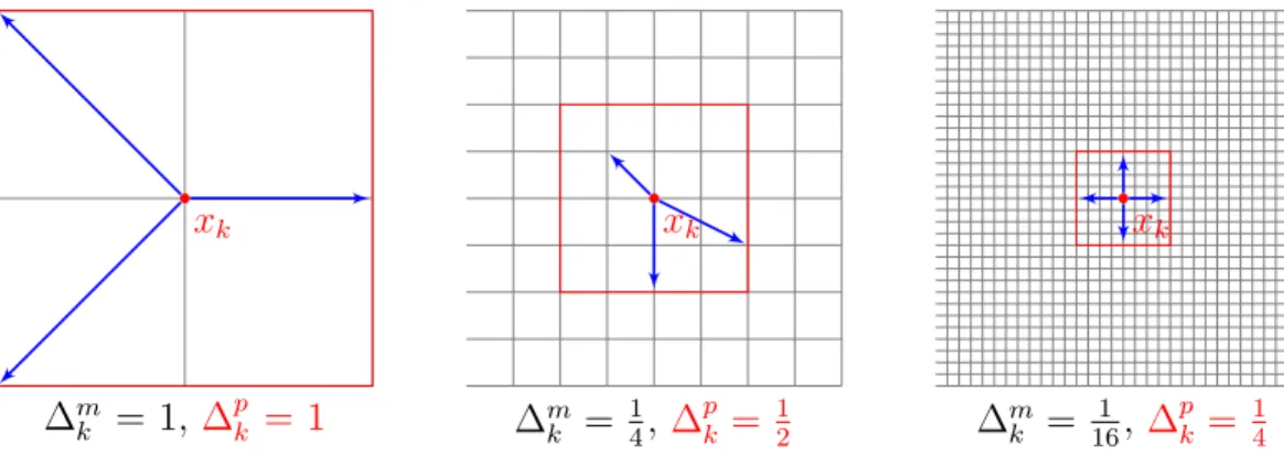
Intuitively, relations between Pk and Mk are shown by examples illustrated in
Figure 2.2 where patterns are represented by arrows with one end at the poll center and the other at a poll point.
xk ∆m k = 1, ∆ p k = 1 xk ∆m k = 1 4, ∆ p k = 1 2 xk ∆m k = 1 16, ∆ p k = 1 4
Figure 2.2 Meshes and poll sets with different sizes
In the definition of a polling set, the introduction of two size-related parameters ∆m
k and ∆ p
k is very important. In GPS the pattern size is totally controlled by only
one parameter that converges to zero when the algorithm samples enough points. In MADS, we control the minimal size (or size unit) by ∆m
k and the maximal size by ∆ p k;
the restrictions on pattern size now are (i) At all iterations, ∆m
k ≤ ∆ p k (ii) lim k∈K∆ m k = 0 ⇔ lim k∈K∆ p k= 0
The new pattern size control principle does not prohibit of pattern size convergence to zero; furthermore, as a result, the MADS poll direction set Dk is no longer a subset
of a predefined set D. In consequence, all the poll directions can form a dense set that indicates that MADS studies thoroughly the neighborhood of the final incumbent.
At the kth iteration, MADS samples the space by performing two steps, Search and Poll. The latter is the crucial step where sampling points are defined by Pk; this
step guarantees the convergence to a first-order local optimum. In the former, a finite set of points on Mk is considered; this is an optional step whose aim is to search for
a global optimum, or to accelerate a solving process by integrating a heuristic based on particular knowledge of the problem. An example of the Search can be found in the work of Audet et al. (2008a).
The convergence of MADS on the blackbox problem minimize
x∈Ω f (x)
is analysed in Audet and Dennis, Jr. (2006) based on the generalized derivatives f◦(x; d) in a direction d, the generalized gradients ∂f (x) and three types of tangent cones (hypertangent cone TH
Ω (ˆx), Clarke tangent cone TΩCl(x), contingent cone TΩCo(ˆx))
defined by Clarke (1983). The analysis shows that MADS generates a converging sequence {xk} that contains a subsequence {xk}k∈K, called the refining subsequence
that satisfies the following conditions:
(i) ∀k ∈ K we have f (xk) ≤ f (x) ∀x ∈ Pk,
(ii) lim inf
k∈K ∆ p
k= lim infk∈K ∆ m k = 0,
(iii) The normalized directions of ˆD = [
k∈K
Dk are dense in the unit sphere.
Thus, the solution ˆx is the limit point of a refining subsequence, ˆx = lim
k∈Kxk.
The convergence hierarchy states that (i) if Ω = Rn (unconstrained optimization):
– if the function f is strictly differentiable near ˆx, then ∇f (ˆx) = 0; – if the function f is convex, then 0 ∈ ∂f (ˆx), where ∂f (ˆx) is subgradient; – if the function f is Lipschitz continuous near ˆx, then 0 ∈ ∂f (ˆx);
(ii) if hypertangent cone TΩH(ˆx) is non-empty:
– then ˆx is a Clarke stationary point of f over Ω: f◦(ˆx; d) ≥ 0, ∀d ∈ TCl Ω (ˆx);
– if f is strictly differentiable at ˆx and if Ω is regular at ˆx, then ˆx is a contingent KKT stationary point of f over Ω: ∇f (ˆx)Td ≥ 0, ∀d ∈ TCo
Ω (ˆx).
A complete description and analysis of MADS can be found in Audet and Dennis, Jr. (2006) while some examples of its extensions can be found in Abramson et al. (2009a); Audet and Le Digabel (2012); Audet et al. (2010b).
NOMAD14 (Le Digabel, 2011) is a C++ software that implements the MADS
algorithm for blackbox optimization under general nonlinear constraints. NOMAD is provided as an executable program or a library corresponding to two modes: batch and library. In the batch mode, users must define their blackbox in the form of an executable that returns output as a list of function values; this mode is intended for
a basic and simple usage. Library mode targets advanced users who require a flexible solver.
Chapter 3
ORGANIZATION OF THE
THESIS
The contributions of this thesis are presented through three papers corresponding to the three following chapters. The present chapter summarizes the works of the three papers in such a way that readers can see our approaches aiming at a parameter tuning framework.
From the reviews of related works in the previous chapter, we can see that the question of parameter tuning is always an important concern; there are many projects but none of them aim at a general framework or a systematical methodology. Hence, our motivation is to propose a framework general enough to apply to virtually all situations, sophisticated enough to take maximum advantage of knowledge of a par-ticular case and flexible to work with other systems. The methodology is initiated by Audet and Orban (2006) with impressive numerical results. The works of this thesis concentrate on developing a framework based on this methodology with three intentions: generality, sophistication and flexibility.
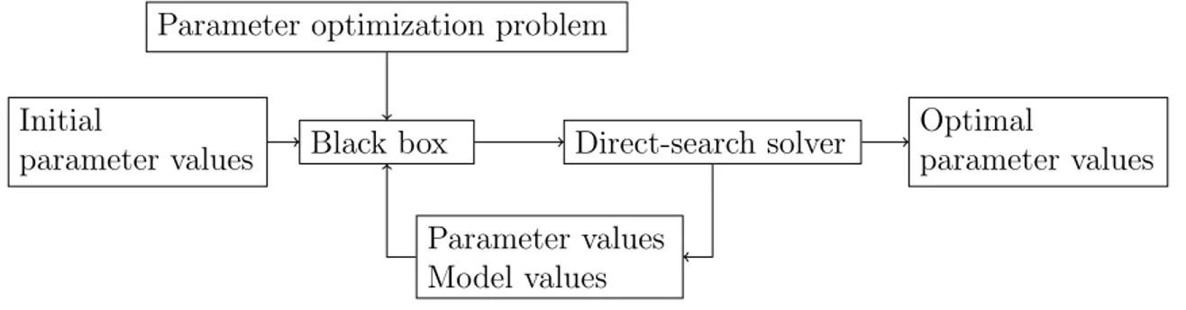
Chapter 4, which corresponds to the publication (Audet et al., 2010a) describes three basic elements that allow launching a tuning session. Although this is a paper that officially introduces the framework, the idea of framework was suggested by Au-det and Orban (2006). The contribution of this paper is that this is the first time that the three fundamental questions of an empirical parameter optimization are studied. The basic elements are next identified; they include parameter description, elemen-tary (atomic) measures, algorithm wrapper, simple parameter constraints, composite measures, model data and model structure. As a consequence, to optimize any algo-rithm, users only need to specify these elements. Within OPAL, these elements are defined by Python syntax in a natural way and a tuning task is described as an opti-mization model composed of variables, model data and model structure. In addition to the framework description, some simple examples of optimizing the DFO algorithm
and numerical results are selectively presented to illustrate OPAL usage and efficiency. After a framework is established, chapter 5 investigates particularities in order to improve the framework. The second paper published in Audet et al. 2011a, illustrates the extensions that target improving framework performance through parallelism and interruption of unnecessary tasks. In the opening part, we show our motivations for parallelizing the tasks. The parallelism is naturally deployed by some particularities of methodology: the core of assessment is to apply the target algorithm over a list of test problems; these applications are independent, thus we can start as many applications as possible at a time; the only constraint is the availability of computational resource. The second place where parallelism can be deployed is the parameter search; although its feasibility depends strongly on the search strategy used. Using NOMAD as the default solver whose parallel working mode is always available, OPAL absolutely has a parallel solver working mode. Taking the advantage of the independence of two stages, assessing the target algorithm and searching the parameter space, OPAL also gives users the possibility of combining two parallelization mechanisms to increase speedup. We deploy the parallelism into OPAL with three working modes and implement it with many techniques behind relating to different parallel platforms such as MPI, LSF or Multi-Threading. However, for OPAL users, parallelism is merely an option in problem definition; that means users can activate by specifying this option a suitable value corresponding to the desired strategy. Besides parallelism, OPAL has another opportunity to accelerate its tuning process with an idea inspired from branch-cutting techniques. We interrupt the target algorithm as soon as an infeasibility is detected. For example, if a parameter optimization requires that the target algorithm returns no error on all 10 test problems, but the target algorithm returned an error on the third problem, there is no need to continue solving the 7 remaining ones, and the entire process may be interrupted. In practice, this technique is neither deterministic nor universal; this means it depends on each concrete problem; it can work with one problem but not with others. Numerical experiment on a trust-region solver, called TRUNK is presented. In the discussion, we propose some directions to apply parallelism more smoothly and more efficiently as well as techniques to increase the probability of interruptions.
Chapter 6 that is in progress paper describes OPAL as a parameter tuning frame-work, as a Python package implementing the framework. In addition to systemat-ically recalling the main characteristics and features, a new feature relating to the