UNIVERSITÉ DE MONTRÉAL
ANALYSIS OF ENERGY SYSTEMS AND PERFORMANCE IMPROVEMENT
OF A KRAFT PULPING MILL
WALID KAMAL
DÉPARTEMENT DE GÉNIE CHIMIQUE ÉCOLE POLYTECHNIQUE DE MONTRÉAL
MÉMOIRE PRÉSENTÉ EN VUE DE L’OBTENTION DU DIPLÔME DE MAÎTRISE ÈS SCIENCES APPLIQUÉES
(GÉNIE CHIMIQUE) AOÛT 2011
UNIVERSITÉ DE MONTRÉAL
ÉCOLE POLYTECHNIQUE DE MONTRÉAL
Ce mémoire intitulé:
ANALYSIS OF ENERGY SYSTEMS AND PERFORMANCE IMPROVEMENT
OF A KRAFT PULPING MILL
Présenté par : KAMAL Walid
en vue de l’obtention du diplôme de : Maîtrise Ès Sciences Appliquées a été dûment accepté par le jury d’examen constitué de :
M. BUSCHMANN Michael, Ph.D., président
M. PARIS Jean, Ph.D., membre et directeur de recherche
Mme. SAVULESCU Luciana, Ph.D., membre et codirectrice de recherche M. FRADETTE Louis, Ph.D., membre
ACKNOWLEDGMENTS
I would like to thank everyone who helped to complete this research project. Special thanks to Mr. Paris and Ms. Savaluscu for their guidance and supervision. In addition, I thank Maryam and Enrique for their time, effort, and patience. I sincerely thank the team at our laboratory for their help and support. Finally, I am filled with gratitude for my parents support and continuous presence during this project.
RÉSUMÉ
Cette étude a pour objectif d’augmenter l’efficacité énergétique d’une usine existante de fabrication de pâte à papier Kraft. Le principal moyen mis en œuvre pour atteindre ce but consiste à développer de nouvelles conceptions optimisées du procédé de fabrication, en d’autre termes il est question ici d’augmenter la récupération interne de chaleur et le taux des fermetures des circuits hydrauliques afin de réduire la consommation énergétique de l’ensemble du procédé. Dans un premier temps il est nécessaire de développer un modèle numérique de l’usine afin d’obtenir les bilans de masses et d’énergie du procédé a l’aide d’un logiciel de simulation de procédés chimiques appelé CADSIM plus® . Ensuite la simulation a été validée par comparaison
avec le fonctionnement réel de l’usine sur les paramètres importants dont la consommation d’eau et de vapeur par des mesures in situ avec le personnel de l’usine. Les écarts relatifs de production et de consommation d’eau et de vapeur sur la totalité des flux de l’usine n’excèdent pas 5 %. La simulation a été caractérisée et comparée aux valeurs moyennes de consommation des usines canadiennes du secteur des pâtes et papiers. Par ailleurs ; les réseaux de vapeur et d’eau de l’usine ont été établis clairement ainsi que les bilans de masse associés. Les profils de température et de consistance de la pâte à papier le long de la ligne de production ont été tracés afin d’identifier les inefficacités énergétiques liées aux points de mélange non isothermiques. L’étude comprend l’analyse des contraintes techniques de l’usine basée sur une approche systématique et documentée. Un manuel technique d’analyse des contraintes a été rédigé, il peut être appliqué à n’importe quelle usine de production de pâte à papier. Les effets potentiels en termes d’économie d’énergie liés aux différents niveaux de contraintes ont été étudiés à l’aided’une analyse globale comprenant l’aspect technique et économique. En terme de re-conception totale du procédé, la ligne A n’a présenté une réduction des consommations que de l’ordre de 2 %, aucune différence remarquable n’a pu être relevée sur la ligne B. Théoriquement la diminution de consommations obtenue sur la ligne A est de 22 % en re-conception totale et 20 % en re-conception partielle. En considérant différentes conceptions du réseau d’échangeur, il est possible d’atteindreune diminution de la consommation de 17 % en re-conception totale et 15 % en re-conception partielle. Pour la ligne B, d’après les courbes composites la diminution théorique de consommation maximale est de 24 % et 16 % d’après la conception du réseau d’échangeur existant.
Une analyse économique a été réalisée à partir du réseau d’échangeurs de la ligne A, elle montre que dans le cas d’une re-conception partielle du procédé, on peut atteindre un temps de retour brut sur investissement de 2,1 ans et de 3,1 ans dans le cas d’une re-conception totale. Ces résultats sont justes si la production de vapeur et la consommation de combustible sont réduites. On peut donc dire qu’il est économiquement rentable d’imaginer une re-conception partielle ou totale de la ligne A de l’usine. Pour la ligne B, la re-conception partielle du réseau d’échangeurs conduit à un temps de retour brut de 3,6 ans si on assure une diminution de la production de vapeur. La solution qui consiste à augmenter la production de vapeur de l’usine afin d’en accroitre la production d’électricité s’est relevée économiquement non rentable pour les lignes A et B.
ABSTRACT
An energy study was done with the objective of improving the energy efficiency of an existing Kraft pulp mill. The improvements have been achieved by developing optimized process designs for the energy systems. The first step was to develop Mass and energy models of the mill on CADSIM plus® software. Second, the model was validated by examining water and steam results and other major parameters. The discrepancy in total steam and water production and consumption was less than 5%. The configuration of the model has been validated directly with the mill staff.
The mill has been characterized and benchmarked against Canadian industry average. In addition, steam and water networks have been built and mass balances around these two systems were done. The temperature and consistency profiles of pulp and water tanks were plotted and inefficiencies due to non isothermal mixing in the process have been identified.
Constraint analysis was performed on the overall mill based on a systematic and documented approach. A set of guidelines have been developed in order to customize the constraint analysis process to any pulp and paper mill. The effect of different constraint levels such as grassroot and retrofit on energy savings has been studied by examining the total savings and economic data. In terms of grassroot and retrofit approaches, it was apparent that in line A the grassroot approach savings were more by 2% while for line B the difference was insignificant. Theoretical savings based on the composite curves for line A were 22% in grassroot and 20% in retrofit. Based on the different heat exchanger network designs, it was possible to achieve 17% savings in grassroot and a maximum of 15% in retrofit. For line B, theoretical savings based on the composite curves were 24% and the potential savings based on the heat exchanger network design was 16%.
An economic analysis was carried where by the heat exchanger networks of line A, show that for the retrofit case, a simple payback period of 2.1 years is achievable while for the grassroot case a simple payback period of 3 years is achievable. This is the case when steam production and fuel consumption are reduced. Therefore, one can say that it is economically viable to design either in grassroot or retrofit constraint level for line A. For line B, the retrofit heat exchanger network was built with a simple payback period of 3.6 years if reducing the steam production is the chosen scenario. Increasing the steam production to produce more electricity was not an economically feasible scenario for both line A and line B.
TABLE OF CONTENTS
ACKNOWLEDGMENTS ... III RÉSUMÉ ... IV ABSTRACT ... VI TABLE OF CONTENTS ... VII LIST OF TABLES ... XI LIST OF FIGURES ... XIII NOTATION ... XVII LIST OF APPENDIXES ... XVIII
CHAPTRE 1 INTRODUCTION AND CONTEXT ... 1
1.1 Problem statement ... 1 1.2 Context ... 1 1.3 Objectives ... 2 1.3.1 General Objective ... 2 1.3.2 Specific Objectives ... 2 1.4 Hypothesis ... 2
1.4.1 Original scientific hypotheses of contribution (OSHC) ... 2
1.4.2 Originality Justification: ... 3
1.4.3 Refutability: ... 3
1.5 Structure and organization ... 4
CHAPTRE 2 LITERATURE REVIEW ... 5
2.1 Kraft Process ... 5
2.2 Methods and techniques ... 8
3.1 Project Phases ... 11
3.2 Breakdown of the phases ... 12
3.3 Definition of the methods, techniques and tools ... 13
CHAPTRE 4 SIMULATION MODEL, VALIDATION AND CHARACTERIZATION ... 15
4.1 Introduction ... 15
4.2 Simulation Model ... 16
4.3 Validation of the model ... 18
4.3.1 Water Validation - Line A ... 19
4.3.2 Water Validation - Line B ... 20
4.3.3 Steam Validation - Line A ... 21
4.3.4 Steam Validation - Line B ... 22
4.3.5 Steam validation - Line A + B ... 23
4.3.6 Other Parameters validation - Line A: ... 24
4.3.7 Other Parameters validation - Line B ... 25
4.4 Characterization of the model ... 26
4.4.1 Steam network ... 27
4.4.2 Water network ... 31
4.4.3 Benchmarking ... 35
4.4.4 Key Performance Indicators ... 38
4.4.5 Pulp line profiles ... 39
4.4.6 Water tanks profiles ... 43
CHAPTRE 5 GUIDELINES TO CONSTRAINT ANALYSIS IN A KRAFT MILL ... 45
5.1 Introduction ... 45
5.2.1 In-depth knowledge of the process ... 47
5.2.2 Identifying and screening the heat transfer points ... 48
5.2.3 Categorizing the type of heat transfer point ... 48
5.2.4 Listing possible energy savings projects ... 59
5.2.5 Identifying possibilities for grassroot and retrofit representations ... 60
5.2.6 Evaluating possible scenarios prior to building composite curves ... 63
5.2.7 Building the composite curves ... 66
5.3 Results ... 67
5.3.1 Water system– Integrated or separated ... 67
5.3.2 Line A and B – Integrated or Separated ... 69
5.3.3 Grassroot approach vs. Retrofit approach ... 72
5.3.4 Identifying all potential energy saving projects ... 79
5.3.5 Building the refined composite curves ... 81
5.3.6 Line A refined composite curves ... 83
5.3.7 Line B refined composite curves ... 84
5.3.8 Summary of refined composite curves ... 85
CHAPTRE 6 HEAT EXCHANGER NETWORKS AND ENERGY SAVING PROJECTS 86 6.1 Introduction: ... 86
6.2 Building the existing heat exchanger network ... 87
6.2.1 Existing heat exchanger network – Line A ... 87
6.2.2 Existing heat exchanger network – Line B ... 90
6.3 Evaluation of energy violations in the existing network ... 92
6.3.1 Energy violations - line A ... 92
6.4 Building the new heat exchanger networks ... 96
6.4.1 Line A - Retrofit – Low savings ... 98
6.4.2 Line A - Retrofit – Medium savings ... 104
6.4.3 Line A – Grassroot - High savings ... 113
6.4.4 Summary of heat exchanger networks –Line A ... 125
6.4.5 Line B – Retrofit – Medium savings ... 126
6.4.6 Summary of heat exchanger network - Line B Retrofit medium ... 137
6.5 Economic Analysis: ... 138
6.5.1 Heat exchanger networks - Line A ... 140
6.5.2 Heat exchanger network - Line B ... 141
CHAPTRE 7 CONCLUSION AND RECOMMENDATIONS ... 142
7.1 Conclusions ... 142
7.2 Recommendations ... 143
BIBLIOGRAPHIE ... 144
LIST OF TABLES
Table 4-1: Major Model information ... 17
Table 4-2: Water validation - Line A ... 19
Table 4-3: Water validation - Line B ... 20
Table 4-4: Steam Production - Line A ... 21
Table 4-5: Steam consumption - Line A ... 21
Table 4-6: Steam production - Line B ... 22
Table 4-7: Steam consumption - Line B ... 22
Table 4-8: Steam production and consumption - Line A and B ... 23
Table 4-9: Other parameters validation - Line A ... 24
Table 4-10: Other parameters validation - Line B ... 25
Table 4-11: Steam balance - Line A ... 28
Table 4-12: Steam balance - Line B ... 30
Table 4-13: Breakdown of water balance – Line A ... 32
Table 4-14: Overall water balance - Line A ... 32
Table 4-15: Breakdown of water consumption - Line B ... 34
Table 4-16: Overall water balance - Line B ... 34
Table 4-17: Key Performance Indicators ... 38
Table 5-1: Initial energy saving projects - line A ... 59
Table 5-2: Initial energy saving projects - line B ... 59
Table 5-3: summary of the composite curves results ... 79
Table 5-4: Line A potential energy saving projects ... 80
Table 5-5: Line B potential energy saving projects ... 80
Table 5-7: Summary of refined composite curves results - Line B ... 85
Table 6-1: List of Existing heat exchanger - Line A ... 89
Table 6-2: List of Existing heat exchangers - Line B ... 91
Table 6-3: Cross pinch violations - Line A ... 93
Table 6-4: Cross pinch violations - Line B ... 94
Table 6-5: Summary of energy saving projects - Retrofit low savings ... 103
Table 6-6: Potential energy savings - Retrofit medium savings ... 112
Table 6-7: Summary of potential energy savings – Grassroot A ... 124
Table 6-8: Summary of savings at different constraint levels – Line A ... 125
Table 6-9: Summary of potential energy saving projects – Retrofit medium B ... 136
LIST OF FIGURES
Figure 2-1: Kraft process overview ... 5
Figure 3-1: Breakdown of the methodology phases ... 12
Figure 4-1: Overall view of the model ... 17
Figure 4-2: Steam network - Line A ... 27
Figure 4-3: Steam network - Line B ... 29
Figure 4-4: Water network - Line A ... 31
Figure 4-5: Water network - Line B ... 33
Figure 4-6: Benchmarking - Thermal consumption ... 35
Figure 4-7: Benchmarking - Water consumption ... 36
Figure 4-8: Benchmarking - Effluent production ... 37
Figure 4-9: Temperature profile - Line A ... 39
Figure 4-10: Consistency profile - Line A ... 40
Figure 4-11: Temperature profile - Line B ... 41
Figure 4-12: Consistency profile - Line B ... 42
Figure 4-13: Warm water and Hot water tanks profile - Line A ... 43
Figure 4-14: Warm water and hot water tanks profile - Line B ... 44
Figure 5-1: Overview of constraint analysis and heat exchanger network methodology ... 47
Figure 5-2: Categorization of constraint type ... 50
Figure 5-3: Constrained Indirect steam Injection - 1a ... 51
Figure 5-4: Non constrained indirect steam injection -1b ... 52
Figure 5-5: Constrained direct steam injection – 1c ... 53
Figure 5-6: Non constrained direct steam injection 1d ... 54
Figure 5-8: Energy in effluents and gases - 3 ... 55
Figure 5-9: Non isothermal mixing in pulp line - 4 ... 57
Figure 5-10: Non isothermal mixing in water tanks - 4 ... 58
Figure 5-11: Retrofit approach ... 61
Figure 5-12: Grassroot approach ... 62
Figure 5-13: Existing water network for line A and line B ... 65
Figure 5-14: Thermal power for Water system - Integrated or separated ... 67
Figure 5-15: Total area for Water system - Integrated or separated ... 68
Figure 5-16: Capital cost for Water system - Integrated or separated ... 69
Figure 5-17: Thermal power for Line A and B – Integrated or Separated ... 70
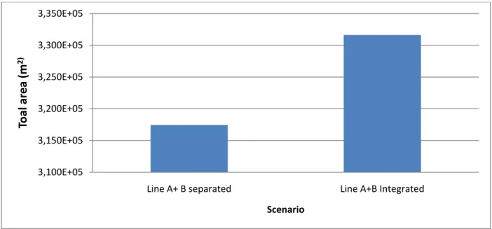
Figure 5-18: Total area for Line A and B – Integrated or Separated ... 70
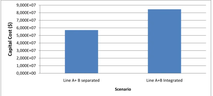
Figure 5-19: Capital cost for Line A and B – Integrated or Separated ... 71
Figure 5-20: Method of obtaining grassroot and retrofit schematic ... 72
Figure 5-21: Line B - Grassroot vs. Retrofit composite curves ... 73
Figure 5-22: Grand composite curve - Line B Process vs. water ... 74
Figure 5-23: Grand composite curve - Close up Line B ... 75
Figure 5-24: Line A - Grassroot vs. Retrofit composite curves ... 76
Figure 5-25: Grand Composite Curve - Process vs. water Line A ... 77
Figure 5-26: Grand composite curve - Close up Line A ... 78
Figure 5-27: Line A - Grassroot After and before refinement ... 83
Figure 5-28: Line A - Retrofit After and before refinement ... 83
Figure 5-29: Line B - Grassroot After and before refinement ... 84
Figure 5-30: Line B - Retrofit After and before refinement ... 84
Figure 6-2: Existing heat exchanger network - Line B ... 90
Figure 6-3: Criss cross violations chart - Line A ... 93
Figure 6-4: Criss cross violations chart - Line B ... 95
Figure 6-5: Project 1 - Bleach Heater ... 98
Figure 6-6: Project 2- Brown Heater ... 99
Figure 6-7: Project 3 - Boiler Air Heater ... 100
Figure 6-8: Project 4- Deaerator Mae up water ... 101
Figure 6-9: Project 5 - Injection 1: Washer 15 ... 102
Figure 6-10: Project 1 - Bleach Heater ... 104
Figure 6-11: Project 2 - Brownstock heater ... 105
Figure 6-12: Project 3 - Boiler Air Heater ... 106
Figure 6-13: Project 4 - Make up Water ... 107
Figure 6-14: Project 5 - Injection 1 Bleaching Washer 15 ... 108
Figure 6-15: Project 6 - Injection 2 – Bleaching Washer 35 ... 109
Figure 6-16: Project 7 – Injection 3 – Washer 45 ... 110
Figure 6-17: Project 8 – Injection 4 – Washer 55 ... 111
Figure 6-18: Project 1& 2 – WW to Washing and Bleaching ... 113
Figure 6-19: Project 3 – Hot water to bleaching ... 114
Figure 6-20: Project 4 – Hot water to Machine ... 115
Figure 6-21: Project 5 & 6 – Hot water to Recausticizing 1 & 2 ... 116
Figure 6-22: Project 7 – Hot water to Bleaching ... 117
Figure 6-23: Project 9 – Make up water (Deaerator) ... 118
Figure 6-24: Project 10 – Injection 1 – Washer 15 ... 119
Figure 6-26: Project 12 – Injection 3 – Washer 45 ... 121
Figure 6-27: Project 13 – Injection 4 – Washer 55 ... 122
Figure 6-28: Project 14 – Boiler Air Heater ... 123
Figure 6-29: Project 1 – Boiler Air Heater B ... 126
Figure 6-30: Project 2 – Make up water (Deaerator) B ... 127
Figure 6-31: Project 3 – Non isothermal mixing in dilution conveyer ... 128
Figure 6-32: Project 4 – Non isothermal mixing in white water tank ... 129
Figure 6-33: Project 5 – Bleach heater and Direct condenser ... 130
Figure 6-34: Pre Project – Elimination of violations in cold blow cooler and green liquor cooler ... 131
Figure 6-35: Project 6 – Injection 1 – Washer 15 B ... 132
Figure 6-36: Project 7 – Injection2 – Washer 35 B ... 133
Figure 6-37: Project 8 – Injection 3 – Washer 45 B ... 134
Figure 6-38: Project 9 – Injection 4 – Washer 55 B ... 135
Figure 6-39: Steam savings economical scenarios Line A ... 140
NOTATION
BL Black Liquor
BLH Black Liquor Heater
BSH Brown stock heater
CBL Cold blow liquor
CBC Cold blow cooler
CL Cooking Liquor
DVSE Dust Vent scrubber exchanger
FS Flashed steam
FSC Flashed steam condenser
FW Fresh Water
GL Green liquor
GLC Green liquor cooler
HW Hot Water
ICC Indirect Contact Cooler
SC Surface Condenser
SWH Shower water heater
WBL Weak black liquor
WL White liquor
LIST OF APPENDIXES
Appendix 1 - Simulation model, validation and characterization ……….147
1.1. Steam network tables 1.2. Injected steam
1.3. Water network tables
Appendix 2 - Guidelines for constraint analysis in a Kraft mill ………..….159
1.1. The complete list of all direct injection steam constraints 1.2. water system data for retrofit and grassroot
1.3. Lists of streams used to build the initial composite curves 1.4. Actual heating requirement
1.5. Information and equations used to evaluate the total area and capital cost 1.6. Water system – separated or integrated composite curves
1.7. Both lines - integrated vs. separate composite curves 1.8. List of streams for non isothermal mixing projects 1.9. List of effluents after refinement
Appendix 3 - Heat exchanger networks and energy saving projects ……….175
1.1. List of streams used for building the heat exchanger network 1.2. Economic analysis data
1.3. List of modified heat exchanger networks and projects for line A 1.4. List of modified heat exchanger networks and projects for line B
CHAPTRE 1
INTRODUCTION AND CONTEXT
1.1 Problem statement
Low paper prices and demand, external competition and high energy costs have caused economic problems for the Canadian pulp and paper industry [1]. As a result, significant efforts are being undertaken to transform the pulp and paper industry into an efficient and profit oriented industry. A pioneer solution that addresses this issue is the retrofitting of biorefineries into existing mills. The implementation of biorefinery options could increase the profitability of the mills by creating a sustainable process with high value secondary products. A key step to be undertaken before the implementation of a biorefinery option is the optimization of a mill with respect to energy and water consumption. Increasing the efficiency of the mill would be achieved in a methodological way that involves a detailed analysis of the energy systems. This could result in steam savings projects scenarios. The promising projects are going to be compared, and analyzed based on technical economic constraints in order to select the potential projects. In addition, the excess steam could be integrated into the biorefinery to insure maximum reutilization of these utilities.
1.2 Context
This project is part of the BioKrEn project whereby 3 mills are being optimized in terms of water and energy. A different biorefinery option will be proposed for each of the optimized mills. The focus will be on the energy optimization of a western Canadian mill. The methodology in this project is adopted from the unified methodology presented in Mateos 2009[2]. In the unified methodology, the method for constraint analysis is based on experience and not a systematic approach for analyzing the constraints and extracting the data to perform pinch analysis. There is a need for a concrete set of guidelines to be followed to achieve realistic theoretical energy targets. A significant section of this project will be involved in developing guidelines for an efficient way to build composite curves and achieve energy targets. These guidelines will build a platform for future energy analysis projects.
1.3 Objectives
1.3.1 General Objective
To improve the energy efficiency of an existing Kraft pulp mill by developing optimized process designs for the energy system.
1.3.2 Specific Objectives
1. Develop and validate a base case simulation for a Kraft mill.
2. Characterize and evaluate the performance of the mill and locate inefficiencies in the process.
3. Perform constraint analysis to develop guidelines for screening between different constraint levels and find theoretical energy targets.
4. Propose potential energy saving projects and develop heat exchanger networks based on techno-economic factors.
1.4 Hypothesis
1.4.1 Original scientific hypotheses of contribution (OSHC)
OSHC: By following the proposed methodology, finding process Inefficiencies and analyzing them will lead to scenarios for reducing steam consumption.
OSHC 1: By using data from a mill, it is possible to develop and validate the simulation. OSHC 2: By benchmarking the mill, it is possible to identify the inefficiencies in the process.
OSCH 3: By extracting the data in grassroot representation, it is possible to increase the theoretical energy saving scope and maintain a similar capital cost to retrofit approach. OSCH 4: By developing heat exchanger networks, it is possible to obtain and evaluate the scope of potential savings and type of projects.
1.4.2 Originality Justification:
OJ: This global and local energy study has not been done on this mill before
OJ 1: Development and validation of the simulation has not been done on CADSIM plus ® software.
OJ 2: This base case mill has not been characterized and evaluated in a detailed manner. OJ 3: The role of data extraction in grassroot and retrofit on the energy savings has not been analyzed in the literature.
OJ 4: The best project for energy savings for the mill has not been determined yet.
1.4.3 Refutability:
RF: If by following the methodology proposed, inefficiencies were not found or the savings were too small to be economically feasible, the hypothesis will be refuted.
RF 1: To be refuted if simulation data differs from the mill data (+/- 10 %)
RF 2: The hypothesis will be refuted if benchmarking doesn’t lead to finding inefficiencies.
RF 3: The hypothesis will be refuted if the grassroot data extraction has no effect on the scope and cost of energy savings when compared to retrofit data extraction.
RF 4: The hypothesis will be refuted if the savings are too small or the projects proposed are not applicable due to economic constraints.
1.5 Structure and organization
In chapter 2, the literature review to support the methods and the findings of this project will be presented
In chapter 3, the overall methodology for energy optimization will be presented. The main focus will be on explaining the different steps in the methodology.
In chapter 4, the results and the techniques used in developing the simulation model, validation, and characterization will be presented.
In chapter 5, constraint analysis results and ideas will be discussed thoroughly and the outcomes of that section will be presented.
In chapter 6, the potential energy saving projects and the heat exchanger networks will be presented. In addition, the economic analysis of the projects and heat exchanger networks will be included.
CHAPTRE 2
LITERATURE REVIEW
2.1 Kraft Process
Chemical pulping was first achieved in the early 1860’s by treating wood with caustic soda. In 1867, advances in the chemical pulping lead to the use of calcium bisulphate as a pulping agent. In the late 1800’s, sulphite pulping had become the dominant pulping method. Towards the end of the century, Kraft pulping was developed. The Kraft process is a chemical process that uses wood chips as feed material to produce pulp and paper products. Kraft pulping produces strong fibres even though it has shorter cooking times than other chemical pulping processes. The advantage of this type is that it is compatible with most types of wood. Wood chips are primarily composed of cellulose, hemicellulose, and lignin. Lignin is a highly organic compound that acts as the glue that keeps the other components intact. Harsh alkaline conditions are required to break down the lignin and free the hemicelluloses and cellulose for the pulp or paper making process. The chemical charge involved is a highly alkaline mixture (pH ~14) of sodium hydroxide (NaOH), sodium sulphide (Na2S) and other sodium compounds used to degrade lignin [3].
The Kraft process has dominated the pulp and paper industry since 1940’s because Kraft mills are able to recycle almost all of the pulping chemicals and have well integrated heat recovery systems. Kraft remains till this day the leading chemical pulping method. The Kraft process overview is presented in figure 2-1. Eight major departments in a Kraft process are needed to produce the final product. These departments are:
Pretreatment
In this department, wood chips are screened to remove large wood pieces and any impurities such as rocks or sand from the feed stream. In addition, the wood chips need to be heated with steam to 130 °C in order to replace the trapped air in chips with steam condensate[3]. This will result in a more efficient impregnation stage due to easier diffusion between impregnation liquor and water. The heated pulp is then sent to the digester in the cooking section.
Cooking
Cooking the pulp is essential to break down and dissolve the lignin to release the cellulosic and hemicellulosic material to produce pulp and paper. Another term for this process is called delignification. This process requires strong alkaline conditions, high temperature and pressure. The alkaline solution used is called white liquor and it mainly consists of NaOH and Na2S. The
cooking temperature is around 160 °C and the pressure is around 1100 kPa[3]. After the cooking stage in the digester, hemicelluloses and cellulose form the pulp while lignin is dissolved in the liquor to form black liquor. The mixtures is washed and cooled down to around 80 °C before it is sent to the washing department.
Washing
Pulp is washed using water or filtrate from bleaching in a cascading manner to separate the lignin from the pulp. The separated lignin forms the black liquor whereby it is sent to the evaporators department. The washed pulp continues to the bleaching department.
Bleaching
In the bleaching department, relatively clean pulp is bleached using chemicals to brighten the pulp into a white color. The bleaching chemicals used are mainly chlorine dioxidedissolved in water, peroxide, and sodium hydroxide. There are many consecutive stages of chemical injection and washing. Hot water, warm water, and fresh water are used to wash the pulp. Acidic effluents and alkaline effluents are released during the bleaching. Finally, clean and white pulp is sent to the forming department.
Forming
The bleached pulp is pressed and formed into sheets before the dryer. The water released from pressing the low consistency pulp is used as a source of water in bleaching. The pressed sheets
are usually dried at two stages; low pressure steam is directly injected in the first stage to increase the temperature of the pulp while in stage two, medium pressure steam is used in an indirect contact dryer. The pulp is produced at a consistency of 90 %.
Evaporators
The black liquor from the washing department enters the evaporators at an average dissolved solid concentration of 19 %. The black liquor is concentrated using low pressure steam in an indirect evaporators operating under vacuum to reach a dissolved solid concentration of 40-50%. The concentrated black liquor is sent to the boilers to be burnt for energy production.
Steam Plant
The black liquor with high concentration of lignin is sent to the recovery boiler to be burnt. The energy from the black liquor is used to produce high pressure steam. The produced steam is sent to a turbine to produce electricity and different levels of steam to be used in the process as a heat source. The spent delignification chemicals at the bottom of the furnace are called the smelt. Smelt is highly concentrated in sodium carbonate and calcium carbonate. The smelt is sent to the chemical recovery department.
Chemical Recovery
Smelt from the recovery boiler is dissolved in water to produce green liquor. Green liquor undergoes chemical reactions to produce the white liquor. The reactions involve the transformation of calcium carbonates into calcium oxides under high temperatures. The calcium oxides are then reacted with sodium carbonates to produce white liquor. The produced white liquor is an alkaline that is mainly composed of sodium hydroxide and sodium sulphide. White liquor is sent to the digesters department thus closing the chemical recovery loop.
2.2 Methods and techniques
The techniques and tools used for process integration and optimization are many. Some include automated optimization paths while other techniques follow a manual path to increase the efficiency of a process [4]. A preliminary step that must be undertaken before any energy study is the development of a reliable base case model that represents a long term average of the operating conditions of a process [5]. The model should include general yet detailed data on the mass and energy balances of the process. Configuration and output data such as steam and water consumption need to be validated to ensure the reliability of the energy analysis [6].
Analyzing the energy and water systems of the mill could be a tedious process if it is not approached in a structured manner. Therefore, evaluating the mill from a general and local perspective will help in channelling efforts to address points of concern in an efficient manner. In other words, the process of benchmarking will reduce the time it takes to locate and analyze points of inefficiencies in an energy audit [7]. Representing the steam and water networks is an essential preliminary step in benchmarking [2]. This will help in locating and identifying the production, utilization and post utilization systems of water and steam. Deepening the understanding of these systems will lead to an easier identification of inefficiencies. Another tool that was mentioned in the literature is the comparison of energy, water, and electricity consumption of a mill with the Canadian average and best practice mills [8, 9]. An energy audit of a Scandinavian mill was performed whereby the mill was compared to the average Scandinavian industry and a state of the art mill. The results showed that excess steam and electricity consumption was higher in the dryers and the evaporators departments of the specific mill. This lead to a preliminary appraisal stating that inefficiencies occurred in both departments and further analysis is required to pinpoint the exact location of the inefficiencies [10].
In the literature, other indicators have been used to evaluate the performance of the process. Calculating and comparing key performance indicators of a mill with the Canadian average was reported to be helpful in identifying general inefficiencies [6]. Some of the key performance indicators include boilers efficiencies, flue gases energy losses, and condensate return [11]. Temperature screening tools are presented in the literature to analyze the consistency and temperature profile across the pulp line as well as the mixing temperatures in water tanks [12]. The outcome of this tool results in the identification of non-isothermal mixing points and direct
heat transfer points in the pulp line and water tanks. By using a temperature vs. enthalpy variation criterion, the relevant points are screened and included in the energy analysis section.
Data handling and extraction is a crucial step that plays a big role on the energy analysis results. The extracted data could have multiple representations and each representation will have an effect on the practicality of the energy savings results. Two main distinct approaches that have not been applied to a Kraft process yet are the grassroot and retrofit representation of data. In the retrofit approach, the streams required are extracted based on the actual conditions and constraints in the mill. On the other hand, grassroot extraction disregards the constraints in the process whereby data is extracted based on final targets. Equipment such as heat exchangers and tanks are not considered as a constraint in the grassroot approach and thus the flexibility of matching hot and cold streams and building an optimized heat exchanger networks will increase [12].
The thermal pinch analysis is a technique that was developed in the late 1980’s to improve the exchange of energy in a process [13]. The principle is fairly simple whereby the hot streams (to be cooled) and cold streams (to be heated) are extracted and plotted on a composite curve. The outcome of this curve includes the minimum heating and cooling requirement, and the possible internal heat recovery based on the design of a new heat exchanger network. The typical savings in the pulp and paper industry based on this principle are between 15%-30% [14]. The water pinch analysis is based on the same principles as thermal pinch analysis. The cold streams become the water sinks and the hot streams become the water sources [15]. The two sets of streams are plotted on a composite curve and the outcome indicates the maximum theoretical water reutilization in a given process. The use of this technique was developed in a manual mode but with the technology advancement, automated optimized algorithms were developed [16]. It is reported that the use of this technique can result in 20-40 % of fresh water reduction [14].
Thermal pinch analysis has been used in the literature to develop energy savings projects. In a case study based on a mill located in eastern Quebec, energy savings were around 20% [2]. On the other hand in the oil and gas industry, energy savings were up to 30 % [14].
A structured approach to retrofitting of heat exchanger networks have been proposed in the literature[17]. A set of general guidelines were developed to aid the engineer in achieving realistic energy targets. The information was very general and therefore a set of guidelines are
needed to the pulp and paper industry. A fairly simple procedure for the design of heat exchanger networks was presented in the literature[18]. Reiteration of the pinch rules and how they should be applied to a new design is covered in this article. Moreover, the idea of assessing the pinch violations was described as well. A more focus article that discusses the retrofitting of an air heating system for a paper making industry represented the practicality of using the simple pinch methods[19]. It was proven that energy savings could be achieved by modifying the heat recovery system. Three heat exchanger networks were designed and evaluated based on their economic prospect.
In order to evaluate different retrofit scenarios in the existing heat exchanger networks, a graphical method is used to examine the possible energy saving scenarios[20]. The focus was on the location of heaters and coolers whereby the closer the coolers and heaters to the pinch, the more cost effective design will be. In the case study, practical results showed the by eliminating Criss-cross violations, higher energy savings are achieved[21]. More work has been done on the elimination of Criss-cross violations whereby a hot stream at high temperature levels is used to heat a cold stream at low temperatures without crossing the pinch[22]. The elimination of these violations as well as the use of an automated program, resulted in heat exchanger network design which have higher energy savings and requires much less time to be obtained.
CHAPTRE 3
METHODOLOGY
3.1 Project Phases
The project consists of four phases. Many techniques, tools and methods are used in each phase to meet the objectives. The phases are listed below:
Phase 1- Development of the simulation and validation:
Phase one will involve the development of a validated base case simulation. Validation of the configuration as well as the output/input data will be carried with the mill staff.
Phase 2 – Characterization:
The second phase involves the characterization and evaluation of the performance of the mill. Points of inefficiencies in the process are going to be identified in this phase.
Phase 3 – Constraint analysis:
The third phase involves the analysis of steam constraints and water constraints before extracting the data to build thermal composite curves. A set of guidelines are developed to provide a systematic approach to obtain theoretical energy targets. The guidelines also include a strategy to shift from theoretical targets to potential energy targets.
Phase 4 – Projects proposal:
In phase four, the existing heat exchanger network is evaluated and further inefficiencies are identified. The proposed projects are implemented into existing heat exchanger network to build new heat exchanger networks at different constraint levels. Economic analysis is done for each constraint level
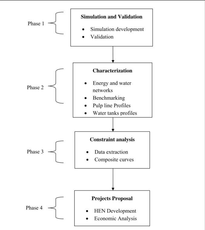
3.2 Breakdown of the phases
Figure 3-1: Breakdown of the methodology phases
Simulation and Validation
• Simulation development • Validation Constraint analysis • Data extraction • Composite curves Projects Proposal • HEN Development • Economic Analysis Characterization
• Energy and water networks
• Benchmarking • Pulp line Profiles • Water tanks profiles Phase 1
Phase 3 Phase 2
3.3 Definition of the methods, techniques and tools
Simulation and validation
A base case simulation will be developed using a pulp and paper software called CADSIM plus®. The simulation will be based on data collected from the mill and will represent the actual
heat and mass balances of the mill for winter conditions. The model will be presented to include the overall production of pulp, consumption of water and steam and fuel. To ensure the reliability of the simulated process, validating major results such as steam and water consumption with average mill data will be undertaken. In addition, the validation of the configuration will be done directly with mill staff.
Characterization:
In the characterization phase, water and steam networks are developed with the relevant stream information. Mass balance around these networks is done to account for all the steam and water production, utilization and post utilization. Key results from the mill will be benchmarked against the Canadian industry average. The results will include total water and energy consumption and effluent production. Key performance indicators such as the efficiency of boilers and the percentage of condensate return will be calculated and compared to the average Canadian industry. In addition, consistency and temperature profiles for the pulp line and water tanks are going to be plotted and examined. The outcome of applying all these tools is to locate energy inefficiencies such as non-isothermal mixing points.
Constraint analysis
The data required for the energy analysis will be extracted in two different ways: grassroot and retrofit. A study will be performed to find out the promising combination of extraction paths. The criteria used to evaluate the path will include minimum utility requirement, heat exchanger area, cost of heat exchanger and the effect on the energy bill. Guidelines will be developed to screen between the different types of extraction in the different process streams.
Using the relative sets of data from step three, thermal pinch analysis will be performed using Aspen Energy Analyzer®. The outcome of the thermal pinch analysis will provide the theoretical minimum heating and cooling required by the mill. This analysis will indicate the scope of the theoretical savings and the potential measures taken to reduce water and energy consumption.
Projects proposal:
Projects to increase the efficiency of the process will be proposed based on the constraint analysis results. The key ideas are going to revolve around increasing internal heat recovery, elimination of non-isothermal mixing points, and elimination of cross pinch transfers to increase the energy savings. The projects will be implemented in new heat exchangers at different constraint levels. The developed heat exchangers networks are going to be compared and evaluated based on the savings, capital cost, operating cost savings, and payback period.
CHAPTRE 4
SIMULATION MODEL, VALIDATION AND
CHARACTERIZATION
4.1 Introduction
In any energy study, streams data consisting of mass and energy information is needed to perform energy analysis. The data could be used directly in the analysis or manipulated and used to build a dynamic mass and energy balance model. The model should be reliable and accurate with output and input data that resembles real life conditions of plants. Therefore the model needs to be validated in terms of output data and configuration. Once the validation is complete, a key step is to characterize and analyze the mill’s energy and water performance and compare it to other existing mills.
This chapter will consist of three main parts; the first part will discuss the simulation model while the second part will discuss the validation process and finally the third part will discuss the characterization of the model/mill. In the first part the idea and the method behind developing a simulation model on CADSIM Plus® will be discussed in details. Followed by that, validation will be presented whereby the main focus is on the validation of configuration and output data. The main data to be validated is water and steam production and consumption. In addition, some other process parameters in the recovery loop will be addressed and validated.
The second part of this chapter will revolve around the idea of mill characterization. This will focus heavily on understanding the water and energy systems. This is a very important step in the methodology and will lead to the identification of inefficiencies in the process. By utilizing water and steam network diagrams, one can notice and identify the different constraints regarding steam consumption. This part of the methodology will be reflected in chapter 5. In addition, benchmarking of the mill’s water and energy consumption as well as other key parameter indicators against the Canadian average will help to identify certain inefficient departments/units. This will help to filter out efficient departments and narrow down the scope of research. Finally, the pulp line temperature and consistency profiles will be presented as well as the hot water and warm water tanks temperature profiles. By examining these charts, non isothermal mixing in the pulp line and water tanks will be identified. Eliminating these inefficient mixing points will increase the energy savings thus making the mill more profitable.
4.2 Simulation Model
The simulation model has been developed on CADSIM Plus® software. It is a specialized program for the pulp and paper industry which creates a model with a mass and energy balance of the process. The model is created using different types of information from the mill. The configuration of the process is primarily based on process and instrumentation diagrams “P&ID’s” as well as distributed control system “DCS” snap shots from the controls room. The input data for the system was based on P & ID’s, DCS snap shots and excel files containing a long term average results for different streams in the process.
The mill consists of two continuous fibre lines operating simultaneously at the same time (Line A and Line B). The mill produces about 1600 oven dry tonne/day at a consistency of 90% or higher to be shipped to Canadian and international consumers. Line A was first built during the late 60’s while line B was constructed during the late 70’s. Both process lines have their own independent fibre lines and recovery loops. The chemical preparation department is shared between them. Each line has a power boiler and a recovery boiler to produce high pressure steam. In each line, high pressure steam is sent to a back pressure turbine to produce electricity and two lower levels of steam. High pressure steam is at 4300 kPa, 400 °C while medium pressure is at 1150 kPa, 202 °C and finally low pressure steam is at 450 kPa, 170 °C. The produced steam has a common header whereby steam is split between both lines based on the requirements of the process. Fresh water is heated through heat exchangers in the process to produce warm water and hot water. During the winter time, fresh water is at 2 °C while warm water is at 50 °C in line B and 57 °C in line A. Hot water is heated to temperatures of 65 °C in line B and 80 °C in line A. Bleaching chemicals are produced from chemical preparation department and sent to line A and line B. There is a continuous exchange of water, chemicals, liquor streams and steam between both lines. The amount of exchange varies depending on the requirement of each line at a specific point in time.
Both lines are almost identical in terms of configuration. In the cooking department, line A has an extra oxygen delignification step that is not present in line B. In addition line B has a two stage atmospheric diffuser while line A has a single stage pressure diffuser. In the evaporators department, line B consists of 6 effect evaporators and a concentrator while line A has a 5 effect
evaporators and a cascade evaporator. Figure 4-1 represents the overall configuration of both lines.
Figure 4-1: Overall view of the model
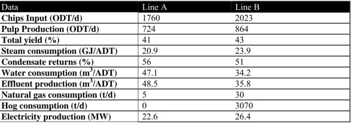
Table 4-1 includes the major information of the model for both lines:
Table 4-1: Major Model informationData Line A Line B
Chips Input (ODT/d) 1760 2023
Pulp Production (ODT/d) 724 864
Total yield (%) 41 43
Steam consumption (GJ/ADT) 20.9 23.9
Condensate returns (%) 56 51
Water consumption (m3/ADT) 47.1 34.2
Effluent production (m3/ADT) 48.5 35.8
Natural gas consumption (t/d) 5 30
Hog consumption (t/d) 0 3070
4.3 Validation of the model
The output/input data and the configuration of the developed model have to be validated thoroughly in order to have an exact representation of the mill’s operating conditions. Working with a validated and reliable model will lead to a practical analysis with applicable results to the mill. Having many discrepancies between the model and mill’s conditions will lead to a faulty analysis with impractical results. Therefore the validation step is a key point that should be done before starting the energy analysis of the mill.
The configuration of the model has to be verified directly with the mill staff. Depending only on P&ID’s or DCS snapshots is not enough to validate the configuration. Major differences could exist between the P&ID’s and the current situation of the mill because of the lack of continuous updates to old P&ID’s. In addition, some of the information from the mill could be unreliable due to errors in measuring devices placed around the mill. Flow meters and consistency meters usually have a high percentage of error that could reach up to 50 % while temperature probes have an accuracy of around +/- 1 °C. In the case where there is a lack of long terms average values of a certain measurement and a discrepancy exist between the model and the mill value, one should suspect that the reason could be from the mill and not the model. In this case, more information is required and that could only be obtained by collaboration with the mill staff.
The input/output data of the model is validated with the mill staff and any other available information source such as DCS snapshots or long term average values on excel files. The best option is to always validate against long term average values if possible. There are three main categories of data to be validated in the mill:
1- Water production and consumption 2- Steam production and consumption 3- Other key parameters
Other key parameters will include flows of certain streams in different departments, temperatures of streams, production of pulp and consumption of white liquor. The validation results for the three categories are presented in the following subsection.
4.3.1 Water Validation - Line A
Water production through heat exchangers and consumption through the many consumers has been validated in table 4-2 against average long term values from the mill. There is a good fit between both sets of data with a difference of less than 5 %. This difference comes from the hot water usage in the pulp machine Slusher and the bleaching white water tank.
Table 4-2: Water validation - Line A
Department/ Consumer Path Model (L/min) Mill (L/min)
Digester – Total 8993 9250
Digester - Cold blow cooler WW to HW Tank 1777 1750
Digester - Flash Steam Condenser WW to HW Tank 7215 7500
Washing – Total 1000 1000
Doctor board shower WW to wire cleaning 1000 1000
Water Production - Make up Water CW to WW tank 1018 2000
Bleaching – Total 13565 14400
Bleaching – Cold
CW to WW bleach
Chest 300 300
Bleaching - doctor board shower WW to wire cleaning 1000 1000
Brownstock dilution conveyer HW 2000 2000
Do Showers HW 4996 5000
Bleach White water chest HW to bleach Chest 2268 3100
washer seal tank D1 HW as Make up 1000 1000
Contaminated condensate tank HW as Make up 2001 2000
Other Consumers HW 1 0
Evaporators – Total 8372 8500
Evaporators - Surface Condenser CW to WW tank 8372 8500
Machine – Total 2619 2190
Machine HW to Washer 429 0
Machine CW to WW Chest 2190 2190
4.3.2 Water Validation - Line B
Water production through heat exchangers and consumption through the many consumers has been validated in table 4-3 against average long term values from the mill. There is a good agreement between both sets of data with a difference of less than 1 %. This difference originates from the fresh water usage in the chemical preparation and the white water in bleaching showers. Table 4-3: Water validation - Line B
Department/ Consumer Path Model (L/min) Mill (L/min)
Digester – Total 11665 12200
Digester - Cold blow cooler CW to WW Tank 3391 3700
Digester - Steam Condenser WW to HW Tank 8274 8500
Washing – Total 3321 1900
Brownstock -doctor board shower WW to wire cleaning 200 200
Brwonstock - Dilution conveyor HW to conveyor 200 200
Brwonstock - Dilution conveyor WW to conveyor 1505 1500
Brwonstock - Press Washer HW 1416 0
Bleaching – Total 12468 9500
Bleaching - Showers White water 4969 2000
Bleaching - doctor board shower WW to wire cleaning 1000 1000
Bleaching Showers HW to showers 6499 6500
Chemical Preparation 3073 7300
Chemical Preparation CW 2978 6000
Chemical Preparation - R8 HW 96 100
Chemical Preparation - R8 Chiller CW 1200
Evaporators 13207 13200
Evaporators - Surface Condenser CW to WW tank 13207 13200
Machine 2023 2000
Machine - White Water Chest CW to WW Chest 500 500
Machine – miscellaneous WW 1523 1500
4.3.3 Steam Validation - Line A
Steam production and consumption have been validated against average long term value and DCS snapshots. By examining table 4-4, one can notice that both the mill and model values have insignificant errors. This can be also said to the MP steam consumed in line A with error equals to 1 %. On the other hand, there is some suspicious discrepancy in the LP consumption and this is due to faulty measurements in the bleaching steam mixers, bleach heater and brown heater flow meters. The reasoning behind this error was obtained through numerous discussions with the mill personnel. The total error in LP steam is 20 %. This information is available in table 4-5.
Table 4-4: Steam Production - Line A
Department Model (t/hr) Mill (t/hr)
Total HP produced 193.8 194 HP Produced-RB1 193.8 194 HP Produced-PB2 0.0 0 HP- From B 0.0 0 HP-to Turbine 268.5 274 HP- to PRV`s 0.0 0 CD – to PRV’s 10.3 11.3
MP produced from turbine 77.6 80
LP produced from turbine 190.9 191
Table 4-5: Steam consumption - Line A
User Model (t/hr) Mill Data (t/hr)
Pulp-MP 10.3 10.15 02 Delignification-MP 5.6 6.4 P.M-MP 50.2 48.5 Evaporators-MP 1.8 1.8 Pulp-LP 13.8 12.75 Bleaching+ brown -LP 26.3 13 Bleach Heater - LP 12.1 3 P.M- Shower - LP 7.5 7.55 P.M- Lazy Shower- LP 24.0 23.95 Evaporator-LP 61.9 62.4
Recovery Boiler- AHX - LP 4.8 2.0
Deaerator-LP 23.5 20
Total MP - Line A 67.9 66.9
4.3.4 Steam Validation - Line B
Steam production and consumption have been validated like line A. By examining the table 4-6, one can notice that both the mill and model values have small errors. MP steam consumed in line B has an error less than 1 %. Moreover, table 4-7 shows some suspicious results in the LP consumption with error of 10 %. Based on the mill personnel experience, the discrepancy is due to faulty measurements in the bleaching steam mixers, heater, and water condenser flow meters. Table 4-6: Steam production - Line B
User Model (t/hr) Mill (t/hr)
Total HP produced 376.5 375 HP Produced-RB5 248.6 248 HP Produced-PB4 127.9 127 HP-to Turbine 292.2 286 HP-to line A 0.0 0 HP- to PRV`s 9.6 9 CD – to PRV’s 10.2 10
MP produced from turbine 62.1 65.9
LP produced from turbine 230.1 232.1
Table 4-7: Steam consumption - Line B
User Model (t/hr) Mill Data (t/hr)
Pulp-MP 29.03 29.95 Pulp Machine-MP 47.81 47.15 Evaporators MP 1.80 1.80 Recovery Boiler -MP 5.00 5.00 ClO2 Plant - MP 1.00 1.00 Digester-LP 27.24 30.50 Bleach Heater-LP 4.68 20.00 Bleaching-LP 26.12 43.00 P.M-LP 25.00 25.00 Evaporators-LP 77.72 78.60 Condensate Stripper - LP 17.00 17.00
Recovery Boiler- AHX - LP 5.93 4.00
Deaerator-LP 51.96 50.00
space heater + vent - LP 19.00 19.00
C.P-LP 6.25 6.85
Water Prod- Cond. - LP 3.81 0.00
Total MP - Line B 84.6 84.9
4.3.5 Steam validation - Line A + B
Table 4-8 represents the total steam production and consumption in both lines. There is an agreement between the production and consumption data. The 30 t/hr that caused the 20% error in line A is consumed in line B. Once the adjustment factor is taken into account, the overall balance of steam production and consumption shows an error of less than 1%.
Table 4-8: Steam production and consumption - Line A and B
Department Model (t/hr) Mill (t/hr)
Total HP Produced 570.3 569 HP Produced-RB1 193.8 194 HP Produced-PB2 0.0 0 HP Produced-RB5 248.6 248 HP Produced-PB4 127.9 127 HP-to Turbine A 268.5 274 HP to turbine B 292.2 286 HP- to PRV's 9.6 9
Total consumption and production
Total MP produced 152.5 151.8 Total LP produced 438.4 438.6 Total MP consumed 152.5 151.8 Total LP consumed 438.4 438.6 Overall Balance CD- TO PRV's ( Steam) 20.5 21.3
Total Steam produced 570.3 569
4.3.6 Other Parameters validation - Line A:
Table 4-9 contains many key parameters located at different streams in the process. The data is validated against snapshots from 2009 and 2010. There is a good fit between both sets of data except in natural gas consumption in RB1 and active alkali concentration in white liquor. Furthermore, the causticizing efficiency is a bit higher in the model than in the mill. All the parameters are presented in table 4-9:
Table 4-9: Other parameters validation - Line A
Department Parameter Mill -
2010
Mill - 2009
Model
Digester A Ratio of organics to inorganic solids in WBL 1.7 - 1.60
Dissolved solids concentration in WBL (%) N/A 18 19 Flow of WBL to evaporators (L/min) 5200 5237 5218
Flow of white liquor (L/min) N/A 2278 2244
Evaporators A Temperature in effect 1 (°C ) 120.5 120.1 119.4 Temperature in effect 2 (°C ) 120.5 119.8 120.2 Temperature in effect 3 (°C ) 110.9 109.5 109.5 Temperature in effect 4 (°C ) 93.5 91.5 91.5 Temperature in effect 5 (°C ) 78.5 75.1 78.8 Temperature in effect 6 (°C ) 58.5 52.2 58.4 Dissolved solids concentration in SBL (%) 45.3 47 54.3 Flow of SBL to recovery boiler (L/min) 1890 1171 1293
Steam Plant A
Make up Water (L/min) 1471 1204
Natural Gas consumption in RB1 (m3/hr) N/A 0.05 0.12
Air flow in RB1 (t/d) N/A 8770 7750
Excess 02 in RB1 (%) N/A 3.7 2.30
Natural gas consumption in PB2 (km3/hr) 0 3.1 0.00
HOG consumption in PB2 0 0 0.00
Recaust A Caustisizing efficiency (%) N/A 79.4 95.0
Active Alkali g/l N/A 104.9 294.2
Sulphidity (%) N/A 29.8 29.8
4.3.7 Other Parameters validation - Line B
Similar to line A parameters, line B parameters portray a good fit between the mill data and the model data. There is a discrepancy in the flow of strong black liquor from the evaporators to recovery boiler. This is due to the high dissolved solids concentration and low water content in the model. All the parameters are presented in table 4-10 below:
Table 4-10: Other parameters validation - Line B
Department Parameter Mill -
2010
Mill - 2009
Model
Digester B Ratio of organics to inorganic solids in WBL 1.7 0 1.75
Dissolved solids concentration in WBL (%) N/A 17 19 Flow of WBL to evaporators (L/min) 6000 5220 5676
Flow of white liquor (L/min) N/A 2405 2366
Evaporators B Temperature in effect 1 (°C ) 114.3 105.3 101.1 Temperature in effect 2 (°C ) 94.7 88 86 Temperature in effect 3 (°C ) 77.6 73.2 79.2 Temperature in effect 4 (°C ) 63.3 62.3 65.2 Temperature in effect 5 (°C ) 56.1 53.8 52.3 Temperature in concentrator (°C ) 116.8 108.6 115.2 Dissolved solids concentration in SBL (%) 70 71 68 Flow of SBL to recovery boiler (L/min) 1389 1327 935
Steam Plant B
Make up Water (L/min) 3888 0 3274
Natural Gas consumption in RB5 (m3/hr) 0.3 0.5 0.12
Air flow in RB5 (t/d) 6960 7147 7247
Excess 02 in RB5 (%) N/A 2.36 2.30
Natural gas consumption in PB2 (km3/hr) 0.0543 0.6 0.12
HOG consumption in PB4 (t/d) 756 490 499
Recaust B Caustisizing efficiency (%) N/A 81.8 95.0
Active Alkali (g/l) N/A 105.3 134.5
Sulphidity (%) N/A 29.1 29.2
Bleaching Bleach rate (t/d) N/A 951 949
LINE A+B Total Machine Prod (adt/d) N/A 1660 1764
Total Digester Prod (adt/d) N/A 1560 1949
4.4 Characterization of the model
The characterization of the validated model is an essential step of the analysis. There are two main outcomes from this step; the first is to enhance the knowledge and understanding of the process while the second outcome is the identification of inefficiencies in the process. In order to achieve these outcomes, the following tools are used:
1- Steam network: A diagram is developed consisting of all steam producers and consumers. In
addition, steam is classified into direct injection and indirect injection. The condensate returning is identified as well. The diagram is supported by a table of stream information.
2- Water network: A diagram is developed consisting of water production and consumption
cycle. In addition, heat exchangers required to heat the water are included. The effluents produced are identified as well. The diagram is supported by a table of stream information.
3- Benchmarking: The mill’s steam consumption, water consumption, and effluent production
are compared against the Canadian industry average. The departments operating below and above the average are highlighted and analyzed.
4- Key Performance Indicators: Certain parameters in the mill are compared to the average Canadian industry. These parameters or indicators include condensate return and boilers efficiency. This will help to indicate where general inefficiencies occur.
5- Pulp line profiles: The temperature and consistency profile along the pulp line have been
plotted. The main idea is to use the diagrams to identify non isothermal mixing in the pulp line. In addition, it presents an excellent image of the consistencies across the line.
6- Water tanks profile: Hot water and warm water tanks flow vs. temperature profiles are
plotted on a chart for input streams and output streams. Non isothermal mixing in tanks could be easily identified. The streams could be shifted between tanks to eliminate non isothermal mixing.
The use of these six tools will shorten the pathway of obtaining energy saving solutions and thus expanding the platform of ideas regarding the energy saving options in the mill. The results from these tools are discussed below.
4.4.1 Steam network
Line A steam network
In 4-2 below, steam production from the boilers and utilization in the different departments have been sketched. To complete the steam cycle, condensate or post utilization has been included in the diagram. In addition, fresh makeup water into the condensate tank has been highlighted. The red streams represent that exchange of HP, MP and LP between line A and line B. The corresponding tables for stream flows and temperatures are in appendix 1-1.
The table below contains the steam balance around the network. The high pressure steam is produced from recovery boiler 1 and is sent to a back pressure turbine. Power boiler 2 is off at this time of the year. Water entering the boilers comes from the deaerator whereby it is heated with low pressure steam. Medium pressure steam and low pressure steam are produced and consumed in the different departments. The total consumption of medium pressure and low pressure steam is 242 t/hr. This steam is either used directly through different injection points in the digester, bleaching, and pulp machine departments or used indirectly through heat exchangers. Indirect steam use is more efficient since the condensate produced is sent back to the condensate collection tank and then the boilers. This will decrease the amount of energy needed to heat the water before the boilers. Information regarding the direct injected steam is presented in appendix 1-2. The condensate returns with a flow of 124 t/hr which is equivalent to 56 % of the total steam consumed. The other 44 % of steam is either directly injected or flashed and used at other points in the process. Medium pressure and low pressure steam is usually flashed to atmospheric conditions before being sent to the condensate collection tank. This occurs in the condensate of medium pressure and low pressure in the digesters, pulp machine, water production, steam plant, and evaporators departments. Directly injected steam flow is 97 t/hr while the flashed steam is 10 t/hr. By combining these values, the steam cycle is balanced. The breakdown of the steam flows in the cycle is presented in table 4-11.
Table 4-11: Steam balance - Line A
Definition Value
Steam consumed (t/hr) 241.5
Condensate return (t/hr) 134 (56%)
Injected steam (t/hr) 97.1
Flashed steam 10.4
Line B steam network
In similar manner to line A, steam production from the boilers and utilization in the different departments have been sketched on figure 4-3. Condensate returning as well as fresh makeup water into the condensate tank has been highlighted on the diagram. The red streams represent that exchange of HP, MP and LP between line A and line B. The corresponding tables for stream flows and temperatures are in appendix 1-1.
The table below contains the steam balance around the network. The high pressure steam is produced from recovery boiler 5 and power boiler 4 and is sent to a back pressure turbine. Medium pressure steam and low pressure steam are produced and consumed in the different departments. The total consumption of medium pressure and low pressure steam is 347 t/hr. This steam is either used directly through different injection points in the digester, bleaching, and pulp machine departments or used indirectly through heat exchangers all over the mill. Direct steam is injected in different streams and equipment such as steaming vessel, water tanks or in the pulp line. The steam injection is a constraint in many cases whereby it cannot be replaced with other hot streams due to operational difficulty. More information regarding the role of steam as a constraint or non constraint will be discussed in chapter 5. In addition, Information regarding the directly injected steam is presented in appendix 1-2. The condensate returns with a flow of 175 t/hr which is equivalent to 51 % of the total steam consumed. The other 49 % of steam is either directly injected or flashed and used at other points in the process.. The directly injected steam flow is 167 t/hr while the flashed steam is 5 t/hr. By combining these values, the steam cycle is balanced. The breakdown of the steam flows in the cycle is presented in the table below:
By comparing line A and line B steam consumption, it is obvious that line A condensate return rates are higher than line B by 5%. A larger amount of directly injected steam is lost in the steaming vessel and the deaerator. In the latter case, a large amount of fresh makeup water enters the condensate tank which needs to be heated in the deaerator using directly injected low pressure steam. This cyclic heating of makeup water and loosing condensate has a negative effect on the efficiency of the cycle. The breakdown of the steam flows in the cycle is presented in table 4-12. Table 4-12: Steam balance - Line B
Definition Value
Steam consumed (t/hr) 346.6
Condensate returns (t/hr) 174.9 (51%)
Injected steam (t/hr) 166.5
Flashed condensate (t/hr) 5.1
4.4.2 Water network
Line A water network
Figure 4-4 below represents the water network in line A. Fresh water (FW) is heated through different heat exchangers across the mill to produce warm water (WW) and hot water (HW). Some of these heat exchangers consume steam while other depends on internal heat recovery to transfer the required energy load. The list of heat exchangers and streams information is presented in appendix 1-3. More information regarding the heat exchanger network is presented in chapter 6. Water is then utilized in the process and sent to the sewer. In addition water from other streams such as chemical solutions in bleaching are included to close the balance.