HAL Id: hal-01609205
https://hal.archives-ouvertes.fr/hal-01609205
Submitted on 5 Sep 2018
HAL is a multi-disciplinary open access
archive for the deposit and dissemination of
sci-entific research documents, whether they are
pub-lished or not. The documents may come from
teaching and research institutions in France or
abroad, or from public or private research centers.
L’archive ouverte pluridisciplinaire HAL, est
destinée au dépôt et à la diffusion de documents
scientifiques de niveau recherche, publiés ou non,
émanant des établissements d’enseignement et de
recherche français ou étrangers, des laboratoires
publics ou privés.
Prediction of the acoustic and bubble fields in insonified
freeze-drying vials
Olivier Louisnard, C. Cogne, S. Labouret, William Montes Quiroz, R.
Peczalski, Fabien Baillon, Fabienne Espitalier
To cite this version:
Olivier Louisnard, C. Cogne, S. Labouret, William Montes Quiroz, R. Peczalski, et al.. Prediction of
the acoustic and bubble fields in insonified freeze-drying vials. Ultrasonics Sonochemistry, Elsevier,
2015, 26, p. 186-192. �10.1016/j.ultsonch.2015.03.008�. �hal-01609205�
Prediction of the acoustic and bubble fields in insonified freeze-drying
vials
O. Louisnard
a,⇑, C. Cogné
b, S. Labouret
b, W. Montes-Quiroz
a, R. Peczalski
b, F. Baillon
a, F. Espitalier
aaCentre RAPSODEE, UMR CNRS 5302, Université de Toulouse, Ecole des Mines d’Albi, 81013 Albi Cedex 09, France bUniversite´ Claude Bernard Lyon 1; LAGEP, UMR CNRS 5007, Campus de la Doua, Bt. CPE, 69616 Villeurbanne, France
Keywords: Acoustic cavitation Bubble structures
Propagation in bubbly liquids Wave attenuation
Sono-freezing Sono-crystallization
a b s t r a c t
The acoustic field and the location of cavitation bubble are computed in vials used for freeze-drying, insonified from the bottom by a vibrating plate. The calculations rely on a nonlinear model of sound prop-agation in a cavitating liquid [Louisnard, Ultrason. Sonochem., 19, (2012) 56–65]. Both the vibration amplitude and the liquid level in the vial are parametrically varied. For low liquid levels, a threshold amplitude is required to form a cavitation zone at the bottom of the vial. For increasing vibration ampli-tudes, the bubble field slightly thickens but remains at the vial bottom, and the acoustic field saturates, which cannot be captured by linear acoustics. On the other hand, increasing the liquid level may promote the formation of a secondary bubble structure near the glass wall, a few centimeters below the free liquid surface. These predictions suggest that rather complex acoustic fields and bubble structures can arise even in such small volumes. As the acoustic and bubble fields govern ice nucleation during the freezing step, the final crystal’s size distribution in the frozen product may crucially depend on the liquid level in the vial.
1. Introduction
Acoustic cavitation has been recognized as a useful method to trigger the nucleation of ice in supercooled water [1–9]. The mechanism underlying this effect at the microscopic scale is still a matter of debate, and two opposite theories exist [10–13]. Inertial cavitation, involving bubbles collapsing radially, is believed to be a necessary condition. However, single-bubble experiments have shown that non-inertial cavitation could also trigger ice nucleation [14], whereas other similar experiments showed the opposite[15].
Whatever the mechanism involved, this phenomenon can be used to control ice nucleation. Ultrasound-induced cavitation allows to trigger ice nucleation at low levels of supercooling, which is unfeasible in normal conditions, owing to the stochastic charac-ter of nucleation. This has incharac-teresting consequences for example in freeze-drying processes, where nucleation at moderate supercool-ing yields larger crystals and therefore enhances sublimation rates
[7,9]. Moreover, controlling the nucleation temperature by ultra-sound allows for inducing ice crystallization simultaneously in all
processed samples and thus for decreasing the dispersion of the crystal properties.
A commonly used industrial freeze-drying system consists of cold shelves, which allow to freeze simultaneously hundreds or thousands of glass vials containing the solution (typically a few mL). Andrieu and co-workers have combined this system with a vibrating plate, which transmits ultrasound to the vials through the vibration of the glass walls[7]. The system has been improved and instrumented, and a design experiment has been performed in order to study the influence of the ultrasonic power and supercool-ing level[9].
Unfortunately, in such experiments, the amplitude and spatial distribution of the acoustic pressure field is generally not known, and the bubble field is difficult to visualize, because of the presence of crystals. This makes the comparison with existing ‘‘single-bubble theories’’ difficult. Empirical correlations between various controllable experimental parameters (frequency, ultrasound amplitude, geometry, type of ultrasonic transducer, temperature) and the observable quantities (nucleation temperature, size and shape of crystals) can be made, but bypassing the knowledge of the acoustic and bubble fields. Yet, it is well known that cavitation fields are never spatially homogeneous and self-organize as local-ized bubble structures[16]. It is therefore interesting to gain more knowledge on the location of the bubbles in the vibrated vials used for freeze-drying of aqueous solutions. Moreover, in order to ⇑Corresponding author.
design and optimize new experimental setups, it would be useful to predict the conditions under which cavitation is really produced in the vial, for example a lower bound on the required vibration amplitude. Predicting the effect of other experimental parameters, such as the filling level in the vials, would also be welcome.
These issues are not specific to sono-crystallization and arise in all applications of acoustic cavitation, for example sonochemistry. Predicting the bubble and acoustic field ab initio has long been thought unfeasible (see[17]for a review), owing to the complexity of the physics involved. However, a recent model of acoustic wave propagation in cavitation fields has shown its ability to capture the main features on some well-known bubble structures[18,19]. In this communication, the latter model is used in the conditions of past sono-freezing experiments in vials[7,9]. The relative simplic-ity of the model is drawn on to vary the experimental parameters.
2. Model
The occurrence of acoustic cavitation is known to produce a self-attenuation of the acoustic field [20,21]. Therefore, correct modelling of acoustics in a cavitating liquid requires to account for the mechanical energy dissipated by the cavitation bubbles. This energy dissipation has two physical origins: thermal conduc-tion in the gas/vapor contained in the bubble, and viscous fricconduc-tion in the violent radial motion around the bubbles. For inertial cav-itation, involving bubble collapses, a correct estimation of these two contributions can only be made on the basis of a real nonlinear bubble dynamics[22].
Under some reasonable approximations, a model accounting for this energy dissipation was proposed[18]. It is based on Caflish equations [23] describing the propagation of a finite-amplitude pressure wave in a dilute bubbly mixture. This model, following the early idea of Foldy[24], expresses the effective pressure field at a given location by adding the average pressure waves radiated by neighboring bubbles to the primary field[25]. The system is closed by a non-linear equation of bubble dynamics, in which the local pressure field acts as the driving term. We emphasize that, by construction, such models do account for the bubble–bubble interaction, and essentially contain the same physics as discrete models of bubble clouds[26–29], which exhibit similar damping phenomena[27]. This issue is discussed briefly in AppendixA.
Since Caflish equations are difficult to solve in the range of acoustic pressures yielding inertial cavitation, they were reduced to a simpler form in[18], by retaining only the fundamental part of the acoustic field pðr; tÞ ¼ PðrÞejxt. The complex amplitude PðrÞ,
which carries the amplitude and phase of the field, was found to approximately obey a nonlinear Helmholtz equation:
r
2P þ k2ð ÞP ¼ 0:jPj ð1ÞThe complex wavenumber can be obtained from:
Rðk2Þ ¼
x
2 c2 l þ 4p
R0x
2Nx
2 0%x
2 ; ð2Þ I k! "2 ¼ %2q
lx
NP
vþP
th jPj2 ; ð3Þwhere
x
is the angular frequency, clthe sound velocity of the pureliquid, and
q
lits density. The quantitiesPvandPthare the averagepower dissipated by the bubble over one acoustic cycle, by viscous friction in the liquid, and by heat conduction in the bubble, respec-tively. The relation between Iðk2Þ and the latter quantities consti-tute the key point of the model, and allow to obtain realistic estimations of the attenuation coefficient of the wave
a
¼ %IðkÞ[22,18].
The bubbles are assumed to have an ambient radius R0. The
bubble density N is assigned to zero in the zones where the acous-tic pressure is less than the Blake threshold, and to a constant value N0in the opposite case.
N ¼ N0 ifjPj > PB 0 ifjPj < PB
#
: ð4Þ
This model has been shown to catch reasonably well the so-called cone bubble structures, visible under large area transducers[30– 32], and the flare-like structures[16]in ultrasonic baths, with some reasonable choices, albeit arbitrary, of the free parameters R0and N0
[19].
Another technical difficulty in acoustic models of sono-reactors is the way solid boundaries are handled. Precedent studies based on linear acoustics showed that modelling the latter by infinitely soft or infinitely rigid boundaries is not convenient [33,34]. Therefore, continuity equations are used to couple the wall vibra-tions to the liquid acoustic field, as detailed in Ref.[34].
In order to calculatePvðjPjÞ andPthðjPjÞ, bubble dynamics
sim-ulations were performed in conditions close to the experiments described in Refs. [7,9]. The bubble dynamics model used was taken from Toegel et al.[35], as in Ref.[18]. The bubbles ambient radius was set to R0¼ 5
l
m, the frequency was f ¼ 35; 890 Hz,the ambient pressure p0¼ 101; 300 Pa, and the driving pressure
jPj was varied between 0:1 p0 and 3 p0. The properties of
supercooled water were taken at %5&C: density
q
l¼ 1000 kg=m3
[36], surface tension
r
¼ 76:3 mN m%1 [37], sound velocitycl¼ 1380 m s%1 [38] and viscosity
l
l¼ 2 ' 10%3Pa s [36]. As inearlier work[18],Pth was found negligible compared toPv and
the latter can be fitted in non-dimensional form by:
P
vðjP(jÞ jP(j2 ¼ p0V0x
exp A þ B tan %1 jP(j % P(0D
P( $ % & ' ; ð5Þwhere p0is the ambient pressure, jPj(¼ jPj=p0is the dimensionless
acoustic pressure amplitude and V0¼ 4=3
p
R30is the bubble ambientvolume. In the considered conditions, the set of fitting parameters in (5) was found to be A ¼ %2:207, B ¼ 5:337, DP(¼ 0:2223,
P(
0¼ 0:9628.
The problem was solved with COMSOL Multiphysics. The geometry and boundary conditions are described in Fig. 1. Axi-symmetry allows to represent only a 2D longitudinal section of the vial. All external solid boundaries were assumed free, except the contact surface between the plate and the vial, where a dis-placement U0 was imposed. The mathematical formulation of
these boundary conditions can be found in Ref.[34]. Finally, the free surface of the liquid was modelled by an infinitely soft wall.
The domains were meshed with triangular elements, whose maximum size was 1 mm in the liquid, and 0.5 mm in the solid. The mesh was refined near the vial bottom because large gradients of acoustic pressure were expected in this zone. Finally, a mesh convergence study has been performed in a typical case, to ensure that the mesh was sufficiently fine.
In all simulations, we considered bubbles of ambient radii R0¼ 5
l
m, yielding the Blake threshold PBof 1:056 p0. The bubbledensity was arbitrary fixed to N0¼ 50 bubbles=mm3. The influence
of these parameters will be discussed below.
3. Results
3.1. Results display.
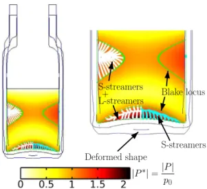
For each simulation case presented hereinafter, all results will be presented as onFig. 2, which is obtained as follows. First, a color plot of the peak dimensionless acoustic pressure jP(j ¼ jPj=p
displayed and the locus of the Blake threshold (P(
B¼ 1:056) is
materialized by a green line. The blue line represents the deformed shape of the vial, at phase
x
t ¼p
, that is, when the contact surface is at its lowest position. Finally, the Bjerknes force field is deduced from the amplitude and phase of the pressure field, as detailed in Ref.[19]. Similarly to the latter reference, the streamlines of this field are sketched as follows, in order to materialize the plausible bubble paths in the liquid:) streamlines are launched from those parts of the solid surfaces where the acoustic pressure exceeds the Blake threshold. These streamlines were named ‘‘S-streamers’’ in Ref.[19], and are dis-played in the right part of the bottle (light-blue online); ) streamlines are launched indifferently from any point where
the acoustic pressure exceeds the Blake threshold (displayed on the left part of the bottle, white lines). This set of streamlines includes the set of S-streamers, and the difference between the two sets are the streamlines originating from the Blake locus. The latter were called ‘‘L-streamers’’ in Ref.[19].
Experiments on cone or flare structures evidenced that S-streamers are always visible, whereas the set of L-S-streamers may be less dense. However, the latter reproduced reasonably well the filamentary structures located near the pressure antinodes, for example in ultrasonic baths. The relation between the Bjerknes force field and the actual location of bubbles remains an open issue, and for now, we chose to present both sets systematically.
3.2. Influence of vibration amplitude
First, the liquid height H was set to 7 mm, as in the experiments of Refs.[7,9], while the vertical displacement U0of the contact
sur-face was varied from 0.009
l
m to 1l
m. The results are displayed onFig. 3, in which a zoom on the liquid has been made for clarity. For the lowest amplitude (upper left plot), the pressure field is everywhere lower than the Blake threshold, so that there are no bubbles, and the acoustic field is essentially predicted by linear acoustics. As the amplitude is increased, the acoustic pressure increases in the bottom zone of the liquid and starts to exceed the Blake threshold. Bubbles can nucleate on the latter and travel toward the vial bottom, which remains attractive (on the three first graphs in Fig. 3). Thus, in this case, no S-streamers are visible. Above U0¼ 0:08l
m (five last graphs inFig. 3), some parts of thevial bottom start to be repulsive for bubbles, because the latter produce a large traveling contribution in the wave [18], which strongly repels bubbles from the solid surface[39,16,40,19], and forms S-streamers [(light-blue online) lines on the right part of
the graph]. As amplitude increases, the S-streamers progressively invade the whole vial bottom and increase in height.
The self-saturation of the field can be clearly seen on Fig. 4, which displays the pressure profiles on the symmetry axis, non-di-mensionalized by
q
lclx
U0, for the eight values of U0used inFig. 3.If the field were given by linear acoustics, all profiles would merge on a universal curve (represented by square symbols). It is seen that for the lowest amplitude U0¼ 0:005
l
m, for which nocav-itation is predicted, the pressure profile indeed merges with this curve. However, for increasing amplitude the dimensionless pres-sure profiles progressively decrease, down to approximately 2% of the universal curve for the highest amplitude U0¼ 1
l
m (lowestcurve on Fig. 4, corresponding to the rightmost bottom plot of
Fig. 3). This clearly illustrates that linear acoustics would predict unrealistic huge values of the acoustic pressure field in the vial.
The displacement amplitude of the vial wall boundaries depends on the point considered and the driving level. It ranges from values close to U0for large drivings, to about 40 U0for low
drivings, where no cavitation occurs (seeSupplementary material, Fig. S1 and caption).
Finally, in the context of sono-freezing, these results for the liq-uid level used in experiments[7,9]yields two important conclu-sions. First, the cavitation field always appears at the bottom of the vial, and this promotes the nucleation of smaller ice crystals in the bottom part. This reinforces the effect of thermal gradients that necessarily arise when the sample is cooled from below[7,41]. This suggests that a different insonification method should be designed if one wish to avoid this synergetic effect, resulting in very broad crystal size distributions. On the other hand, because of self-sat-uration, it can be seen that a large increase of the driving amplitude does not produce large variations neither of the acoustic field ampli-tude, nor of the cavitation field extension. There might be therefore an optimum amplitude level sufficient to trigger ice nucleation.
3.3. Influence of liquid height
For a given amplitude U0¼ 1
l
m, the liquid height has beenvaried between 6 mm and 20 mm. The resulting acoustic field Fig. 1. Geometry and boundary conditions of the vial filled with liquid. The liquid
level H is measured from the on-axis inner side of the vial wall.
Fig. 2. Example of simulation results (U0¼ 1lm , H ¼ 16 mm, f ¼ 35; 890 Hz). The
right graph is a zoom on the left one. Color plot: peak dimensionless acoustic pressure jP(j ¼ jPj=p
0. Lines on the left part of figure (white): streamlines of the
Bjerknes force field launched from any point where the Blake threshold is exceeded. Lines on the right part of figure (light-blue): streamlines of the Bjerknes force field launched from any solid surface where the Blake threshold is exceeded. The line limiting the former set of streamlines materializes the Blake threshold locus (green). The deformed shape of the glass wall is also represented (blue) at phase xt ¼p. (For interpretation of the references to colour in this figure legend, the reader is referred to the web version of this article.)
and bubble paths are represented onFig. 5. Above a critical liquid level, the region where the Blake threshold is exceeded splits in two parts (from H ¼ 10 mm and above onFig. 5). A dome-shaped region appears on the vial bottom, and a toroidal region builds up along the vertical glass wall, with a pressure antinode against the wall. The latter remains approximately at a constant distance from the liquid free surface as the level is increased. The stream-lines in this region show that a classical streamer can be formed, with bubbles attracted by the wall pressure antinode. Conversely, at the vial bottom, the shape of S-streamers show that the wall is
repulsive for the bubbles in a dome-shaped region extending almost up to the Blake locus.
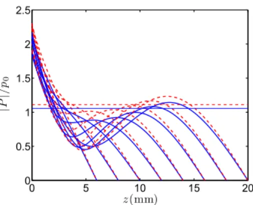
On the two last graphs ofFig. 5(H = 18 and 20 mm), it can be seen that the Blake threshold is exceeded in a small region on the axis, so that the toroidal region finally fills in the whole width of the vial. This occurs because the liquid level is large enough to enable the formation of a longitudinal standing wave, as evidenced by the axial pressure profiles displayed on Fig. 6 (solid lines). Moreover, for the largest level (H = 20 mm), it can be seen that a very small conical S-streamer appears near the wall, which means that the latter becomes repulsive. This is due to the fact that in this small region, the bubble dissipation becomes large enough to con-vert the local standing wave into a radial traveling wave. A zoom on the potentially resulting structure is displayed onFig. 7, where streamlines of the Bjerknes force field have been launched from arbitrary points. The result shows some similarity with the flare structures described in Refs.[16,19].
These results suggest that changing the supercooled liquid level in the vial can have important consequences on the bubble field, and therefore on ice nucleation locations, and finally on the crys-talline structure of the frozen product. The bubble structure appear-ing near the wall for high levels, exemplified inFig. 7, may trigger ice nucleation in this region. In such a case, one would expect that the freezing front would not only travel upwards from the vial bot-tom, as observed in past experiments, but that another front would start from the vertical walls and travel towards the vial axis. This should have visible consequences on the morphology of ice crystals Fig. 3. Acoustic field and bubble paths for increasing driving amplitudes U0and a water level H ¼ 7 mm, at f ¼ 35; 890 Hz. The figures zoom on the liquid for clarity. From left
to right and top to bottom: U0¼ 0:005; 0:02; 0:05; 0:08; 0:1; 0:2; 0:5; 1lm. SeeFig. 2for description.
Fig. 4. Dimensionless acoustic pressure along the symmetry axis, in the conditions ofFig. 3. From top to bottom: U0¼ 0:005; 0:02; 0:05; 0:08; 0:1; 0:2; 0:5; 1lm. The
squares (merging exactly with the curve U0¼ 0:005lm) correspond to the universal line predicted by linear acoustics.
H = 20 mm H = 8 mm H = 10 mm H = 12 mm H = 14 mm H = 16 mm H = 18 mm
H = 6 mm
Fig. 5. Acoustic field and bubble paths for an amplitude U0¼ 1lm and a liquid level H ¼ 6 mm;8 mm;10 mm;12 mm;14 mm;16 mm;18 mm;20 mm from left to right, at f ¼ 35; 890 Hz. SeeFig. 2for description. For readability, the color plot is restricted to 4 levels, corresponding to jP(j in the intervals (from lightest to darkest shade): ½0; P(
B+,
½P(
nucleated in this region. A specific experimental campaign should be performed in order to confirm these predictions.
3.4. Influence of parameters R0and N0
The calculations of Section3.3 have been repeated in exactly the same conditions, but assuming bubbles of ambient radius R0¼ 3
l
m. The resulting axial pressure profiles are representedwith dashed lines onFig. 6. They are slightly larger than the ones obtained for R0¼ 5
l
m, but their global evolution for increasingliquid levels remains unchanged.
On the other hand, the calculations were repeated for R0¼ 5
l
m, H = 16 mm, U0¼ 1l
m, and varying the bubble densityN0from 20 to 200 bubbles/mm3by steps of 30. Similar ranges of
bubble densities have been reported in bubble clouds under horn-type transducers [27]. As expected, the resulting pressure profiles along z (Fig. 8) decrease for increasing N0, which is the
logi-cal consequence of an increased interaction between bubbles as they are more densely distributed. However,all profiles onFig. 8
maintain the same shape. It can be noted that for the lowest bubble density (N0¼ 20 bubbles=mm3), the Blake threshold is exceeded
near z ¼ 10 mm, because less bubbles produce less wave
attenuation. This means that keeping all parameters constant, lower bubble densities would favor the appearance of the bubble structure in the middle of the liquid (similar to the ones visible on the two rightmost graphs of Fig. 5). This result is interesting and rather counter-intuitive, and suggests that in some config-urations, injecting less bubbles in the model yields more bub-bles-populated regions in the liquid.
4. Conclusions
Calculations of the acoustic and bubble fields have been per-formed in a vial insonified from the bottom by a vibrating plate, in the conditions of past sono-freezing experiments. The results confirmed that the bubble field was located at the bottom of the vials for low liquid levels, but evidenced also a more complex, non trivial bubble structure as the liquid level increases. Although these results must be validated against experiments, it has been demonstrated that even in such small samples involved by freezing aqueous solutions in glass vials, spatial variations of the crystal sizes and shapes may occur because of the inhomogene-ity of the acoustic and bubble fields. The knowledge of the latter cannot therefore be disregarded in such experiments. The influ-ence of other parameters, such as the clamping of some part of the vial, could also be studied. On the other hand, it has been shown that linear acoustics calculations yield unrealistic predic-tions in such problems.
Acknowledgments
The authors acknowledges the support of the French Agence Nationale de la Recherche (ANR), under grant SONONUCLICE (ANR-09-BLAN-0040–02) ‘‘Ice nucleation control by ultrasounds for freezing and freeze-drying processes optimization’’.
Appendix A. On the bubble–bubble interaction in the model Following a suggestion of a reviewer, this appendix examines whether the model used in this paper, which is a simplified version of Caflish equations[23], accounts in some way for the interaction between bubbles, as do ‘‘discrete’’ models describing the mutual influence of bubbles oscillating in pairs [26] or in clusters [27]. This discussion intends to clarify briefly and as simply as possible this issue, at the price of mathematical rigor. The main lines of the discussion are borrowed to Prosperetti[25].
Fig. 6. Acoustic pressure profile along the symmetry axis, in the conditions ofFig. 5. Solid lines (blue): R0¼ 5lm; dashed lines (red): R0¼ 3lm. All curves end at z ¼ H
and are therefore self-explanatory. The horizontal thin lines indicates the respective Blake thresholds for R0¼ 5lm and R0¼ 3lm. (For interpretation of the references
to colour in this figure legend, the reader is referred to the web version of this article.)
Fig. 7. Zoom on the flare-like structure appearing near the vial wall for H ¼ 20 mm (rightmost graph onFig. 5). The slanted lines (green) are the Blake loci. The vial wall is represented in gray. (For interpretation of the references to colour in this figure legend, the reader is referred to the web version of this article.)
Fig. 8. Acoustic pressure profile along the symmetry axis, at f ¼ 35; 890 Hz, for U0¼ 1lm, H ¼ 16 mm, and a bubble density N0¼ 20; 50; 80; 110; 140;
170; 200 bubbles=mm3(from top to bottom). The horizontal thin line indicates
Interacting bubble models, such as Eq. (7) in[26], or Eq. (2) in the cluster model of Yasui and co-workers[27], consist in a bubble radial dynamics equation written as:
R€R þ32_R2¼1
q
l pL% pSðr; tÞ % p1 ð Þ %X N%1 i¼1 1 di 2 _R 2 iRiþ R2i€Ri ! " ; ðA:1Þwhere for simplicity, we have omitted refining terms accounting for liquid compressibility and for water evaporation/condensation at the bubble wall. The first line in Eq.(A.1) is a classical Rayleigh equation, where R is the bubble radius,
q
l is the liquid density, pLis the pressure in the liquid at the bubble wall, pSðtÞ ¼ pAðrÞ sin
x
tis the driving acoustic pressure field at the bubble centroid location r if the latter were absent, and p1is the static pressure. The
addi-tional term in the second line of Eq.(A.1)describes the pressure fields radiated by N % 1 neighboring bubbles, among which the iest one is located at a distance di from the bubble described by(A.1),
and has an instantaneous radius RiðtÞ.
Eq. (A.1)therefore states simply that the ‘‘effective’’ pressure field driving the described bubble is basically:
peffðr; tÞ ¼ pSðr; tÞ þ
q
l XN%1 i¼1 1 di 2 _R 2 iRiþ R2iR€i ! " : ðA:2ÞAssuming further that the N % 1 other bubbles are identical, their dynamics RiðtÞ are solutions of equations formally similar to
(A.1). Furthermore, assuming that bubbles are numerous enough so that they can be described by a bubble density nðr0Þ, and noting
that 2 _R2R þ R2R ¼ €V=4€
p
, the discrete sum in Eq. (A.2) can be replaced by a volume integral:peffðr; tÞ ¼ pSðr; tÞ þ
q
lZZZV
€ Vðr0; tÞ
4
p
jr % r0jnðr0Þdr0; ðA:3Þwhere Vðr0; tÞ is the instantaneous volume of the (numerous)
bub-bles located at r0.
Now, having in mind a model describing the spatial variations of peff, we note that the Green function for the Laplacian can be
readily recognized in the integral, so that taking the Laplacian of Eq.(A.3), we get:
r
2peffðr; tÞ ¼r
2pSðr; tÞ %q
l ZZZ V € Vðr0; tÞdðr % r0Þnðr0Þdr0 ¼r
2pSðr; tÞ %q
lnðrÞ @2V @t2ðr; tÞ;where d stems for the Dirac function. In this equation, pS is the
acoustic pressure field that would drive the bubble if it were alone (in absence of interaction), and satisfies therefore a standard linear propagation equation in the pure liquid. Thus, the above equation finally writes: 1 c2 l @2pS @t2 ðr; tÞ %
r
2p effðr; tÞ ¼q
lnðrÞ @2V @t2ðr; tÞ;where clis the sound velocity in the pure liquid. If we replace pSby
peff in the first term of the LHS of this equation,1we get exactly the
first equation of the Caflish model ([23,42]):
1 c2 l @2peff @t2 ðr; tÞ %
r
2p effðr; tÞ ¼q
lnðrÞ @2V @t2ðr; tÞ; ðA:4Þof which our model is an approximation (see Ref.[18]for details). The Caflish model is then closed by calculating the bubble vol-ume Vðr; tÞ ¼4
3
p
R3ðr; tÞ from a bubble dynamics equation drivenby the local effective pressure field peffðr; tÞ, exactly in the same
way as in(A.1), Riis calculated as a solution of(A.1)itself!
The continuous path between the two approaches summarized above shows that the bubble interaction is indirectly included in our model (as for any model derived from Caflish equations), but in a global fashion. As detailed in[18], what we call ‘‘the acoustic field’’ is the first harmonic part of the effective field peff from
(A.4), or from (A.1). It is spatially damped because as shown in
[18], part of the effective field energy is dissipated by viscous fric-tion in the radial mofric-tion of the liquid around the bubbles (and to a lesser extent by heat transfer in the bubble).
As a final comment, these remarks might also shed light on one major result of Ref.[27](Section V and Fig. 6). It is found there that the actual pressure profile on the axis (solid line) is far less than that predicted by the analytical solution of linear acoustics for a circular piston [Eq. (15) in the latter reference]. This is exactly the result that we obtain in all the simulations with our model, either in the present paper (seeFig. 4), or in Ref.[18](Fig. 6). We suggest therefore that in Section V of Ref.[27], if the peak value of peffðxÞ from Eq.(A.2)had been evaluated instead of paðxÞ, the
authors might have recovered values close to the solid line of their
Fig. 5.
Following the same line of reasoning, we also note that if we were to reproduce Figs. 9–11 of Ref.[27]with our model, we would obtain the dashed line by driving the bubble with the linear acous-tic prediction pSðtÞ, and the solid line by driving the bubble with
the pressure field peffðtÞ calculated with our model.
We conclude therefore that both approaches contain in fact the same physics, and that our model (being a derived product of Caflish Model) catches the bubble–bubble interaction at least approximately. The informal comments of this appendix would probably deserve to be revisited more thoroughly, and possibly extended to more complex configurations, such as mixtures of bubbles of different sizes [29]. This may motivate a dedicated study. We thank the reviewer for suggesting this interesting discussion.
Appendix B. Supplementary data
Supplementary data associated with this article can be found, in the online version, athttp://dx.doi.org/10.1016/j.ultsonch.2015.03. 008.
References
[1]S.L. Hem, Ultrasonics 5 (4) (1967) 202–207. [2]J.D. Hunt, K.A. Jackson, Nature 211 (1966) 1080–1081. [3]T. Bhadra, Indian J. Phys. 42 (2) (1968) 91.
[4]S.N. Gitlin, S.S. Lin, J. Appl. Phys. 40 (12) (1969) 4761–4767.
[5]T. Inada, X. Zhang, A. Yabe, Y. Kozawa, Int. J. Heat Mass Transfer 44 (23) (2001) 4523–4531.
[6]R. Chow, R. Blindt, R. Chivers, M. Povey, Ultrasonics 43 (4) (2005) 227–230. [7]K. Nakagawa, A. Hottot, S. Vessot, J. Andrieu, Chem. Eng. Process. 45 (9) (2006)
783–791.
[8]B. Lindinger, R. Mettin, R. Chow, W. Lauterborn, Phys. Rev. Lett. 99 (4) (2007) 045701.
[9]M. Saclier, R. Peczalski, J. Andrieu, Chem. Eng. Sci. 65 (10) (2010) 3064–3071. [10]J.D. Hunt, K.A. Jackson, J. Appl. Phys. 37 (1966) 254–257.
[11]R. Hickling, Nature 206 (1965) 915–917.
[12]C.P. Lee, T.G. Wang, J. Appl. Phys. 71 (1992) 5721–5723. [13]R. Hickling, Phys. Rev. Lett. 273 (1994) 2853–2856.
[14]R. Chow, R. Mettin, B. Lindinger, T. Kurz, W. Lauterborn, in: D.E. Yuhas, S.C. Schneider (Eds.), Proceedings of the IEEE International Ultrasonics Symposium, vol. 2, IEEE, 2003, pp. 1447–1450.
1 This assumption is linked to an hypothesis of dilute liquid-bubble mixture, in
[15]K. Ohsaka, E.H. Trinh, Appl. Phys. Lett. 73 (1) (1998) 129–131.
[16]R. Mettin, in: A.A. Doinikov (Ed.), Bubble and Particle Dynamics in Acoustic Fields: Modern Trends and Applications, Research Signpost, Kerala (India), 2005, pp. 1–36.
[17]I. Tudela, V. Sáez, M.D. Esclapez, M.I. Díez-García, P. Bonete, J. González-García, Ultrason. Sonochem. 21 (3) (2014) 909–919.
[18]O. Louisnard, Ultrason. Sonochem. 19 (2012) 56–65. [19]O. Louisnard, Ultrason. Sonochem. 19 (2012) 66–76.
[20]L.D. Rozenberg, in: L.D. Rozenberg (Ed.), High-Intensity Ultrasonic Fields, Plenum Press, New-York, 1971.
[21]M.M. van Iersel, N.E. Benes, J.T.F. Keurentjes, Ultrason. Sonochem. 15 (4) (2008) 294–300.
[22] O. Louisnard, Congress on Ultrasonics, Santiago de Chile, January 2009, Phys. Procedia 3 (1) (2010) 735–742.
[23]R.E. Caflish, M.J. Miksis, G.C. Papanicolaou, L. Ting, J. Fluid Mech. 153 (1985) 259–273.
[24]L.L. Foldy, Phys. Rev. 67 (3–4) (1944) 107–119.
[25]A. Prosperetti, in: S. Morioka, L. van Wijngaarden (Eds.), IUTAM Symposium on Waves in Liquid/Gas and Liquid/Vapour Two-Phase Systems, Kluwer Academic Publishers, 1995, pp. 55–65.
[26]R. Mettin, I. Akhatov, U. Parlitz, C.D. Ohl, W. Lauterborn, Phys. Rev. E 56 (3) (1997) 2924–2931.
[27]K. Yasui, Y. Iida, T. Tuziuti, T. Kozuka, A. Towata, Phys. Rev. E 77 (1) (2008) 016609.
[28]K. Yasui, J. Lee, T. Tuziuti, A. Towata, T. Kozuka, Y. Iida, J. Acoust. Soc. Am. 126 (3) (2009) 973–982.
[29]K. Yasui, A. Towata, T. Tuziuti, T. Kozuka, K. Kato, J. Acoust. Soc. Am. 130 (5) (2011) 3233–3242.
[30] A. Moussatov, C. Granger, B. Dubus, Ultrason. Sonochem. 10 (2003) 191–195. [31]C. Campos-Pozuelo, C. Granger, C. Vanhille, A. Moussatov, B. Dubus, Ultrason.
Sonochem. 12 (2005) 79–84.
[32]B. Dubus, C. Vanhille, C. Campos-Pozuelo, C. Granger, Ultrason. Sonochem. 17 (2010) 810–818.
[33]K. Yasui, T. Kozuka, T. Tuziuti, A. Towata, Y. Iida, J. King, P. Macey, Ultrason. Sonochem. 14 (2007) 605–614.
[34]O. Louisnard, J.J. González-García, I. Tudela, J. Klima, V. Saez, Y. Vargas-Hernandez, Ultrason. Sonochem. 16 (2009) 250–259.
[35]R. Toegel, B. Gompf, R. Pecha, D. Lohse, Phys. Rev. Lett. 85 (15) (2000) 3165– 3168.
[36]P.G. Debenedetti, J. Phys. Condens. Matter 15 (45) (2003) R1669. [37]D. Kashchiev, J. Chem. Phys. 125 (4) (2006) 044505.
[38]E. Trinh, R.E. Apfel, J. Acoust. Soc. Am. 63 (3) (1978) 777–780.
[39] P. Koch, D. Krefting, T. Tervo, R. Mettin, W. Lauterborn, in: Proc. ICA 2004, vol. Fr3.A.2, Kyoto, Japan, 2004, pp. V3571–V3572.
[40] R. Mettin, in: T. Kurz, U. Parlitz, U. Kaatze (Eds.), Oscillations Waves and Interactions, Universitätsverlag Göttingen, 2007, pp. 171–198.
[41]A. Hottot, S. Vessot, J. Andrieu, Chem. Eng. Process. 46 (7) (2007) 666–674. [42]K.W. Commander, A. Prosperetti, J. Acoust. Soc. Am. 85 (2) (1989) 732–746.