Trade Liberalization, Inequality and Poverty in Brazilian States

This version: August 10th, 2009

Trade Liberalization, Inequality and Poverty in Brazilian States

Abstract

This paper studies the impact of trade liberalization and international trade on household income inequality and poverty using detailed micro-data across Brazilian states, from 1987 to 2005. Results suggest that Brazilian states that were more exposed to tariff cuts experienced smaller reductions in household poverty and inequality. If significance of results on Brazilian states depends on the choice of poverty and inequality indicators, robust and contrasting results emerge when we disaggregate into rural and urban areas within states. Trade liberalization contributes to poverty and inequality increases in urban areas and may be linked to inequality declines in rural areas (no significant effect on rural poverty appears from our study). In terms of observed integration to world markets, import penetration plays a similar role as trade liberalization for Brazilian states as a whole. On the contrary, rising export exposure appears to have significantly reduced both measures of household welfare.

Keywords: Trade liberalization, poverty and inequality; Brazil states. JEL codes: D31, F16, F14

1. Introduction.

The effects of globalization on income distribution continue to be one of the most discussed topics in academic and policy circles. Back in the eighties, the policy debate essentially involved industrialized countries seized by rising inequalities and increased international

*

Marta Menéndez is at LEDa, Université Paris-Dauphine and at PSE (INRA); Aude Sztulman is at LEDa, Université Paris-Dauphine and CEE, Marta Castilho is at Universidade Federal Fluminense and benefited from financial support from CAPES (Brazil). Correspondence to Aude Sztulman, Université Paris-Dauphine, Place du Maréchal de Lattre de Tassigny, 75 775 Paris cedex 16, France. E-mail: Aude.Sztulman@dauphine.fr. The authors are particularly indebted to Nina Pavcnik for careful reading and thoughtful comments. This paper has benefited from helpful discussions with Barbara Coello, Jean-Marc Siroën and participants at conferences and seminars. The authors are grateful to Honorio Kume for kindly providing us with tariffs data and to Pierre-Emmanuel Couralet and Jeremie Gignoux for their help in building harmonized data series from PNAD surveys.

competition in domestic markets. Since then, the implementation of trade reforms in several developing and emerging countries and the growing availability of datasets has led to more studies on the distributional and social effects of international trade in countries from the developing world. The debate is partially motivated by the complexity of the channels through which globalization - an all-purpose term here used to describe trade liberalization and integration to world markets - affects inequality as well as poverty within a country (see Goldberg and Pavcnik, 2004, 2007; Winters et alii, 2004; Ferreira et alii., 2007a, for a survey on the various trade-transmission mechanisms).

In this paper we study the impact of trade liberalization and international trade on household income inequality and poverty using detailed micro-data across Brazilian states, from 1987 to 2005. We seek to measure whether, within Brazil, states that experienced a greater degree of exposure to trade during the past two decades exhibited differential changes in their income distribution, both in poverty and inequality levels.

This paper makes several contributions to the literature on globalization and income distribution. First of all, using sub-national units of observation (in our case, the Brazilian states, together with a distinction between rural and urban areas within states), this study performs an analysis taking into account regional differences in the Brazilian economy. By taking this regional approach, our paper puts up to a recent strand of research that includes the spatial dimension in the study of the impact of trade liberalization on income distribution within a country (see Wei and Wu, 2002, on China; Topalova, 2005, on India; McCaig, 2009, on Vietnam; Nicita, 2004 on Mexico).1

Second, the distributional measures considered in this paper are broader than those usually looked at in the literature. Though ultimately trade reforms should affect household welfare, it is only recently that a few studies have considered measures beyond wage inequality and skill premium (Topalova, 2005; Porto, 2003, 2006; Ferreira et alii., 2007a; McCaig, 2009). The focus of the literature on skill premium is not surprising and essentially derives from the predictions of the classical Heckscher-Ohlin-Samuelson (HOS) model. According to the HOS model, in poor countries, usually considered as relatively well endowed in unskilled

1

Another branch of the literature, recently developed, studies whether incomes or wages are higher in regions with access to larger markets for their goods, using new economic geography models (see for example, Hanson, 2005; Redding and Venables, 2004; Fally et alii., 2008).

labor, trade liberalization should raise relative demand for this factor and consequently, lower wage inequality and eventually reduce poverty. These predictions of the HOS theory of international trade have nevertheless been challenged by empirical works on some Latin American countries, where a combination of rising skill premium and a deterioration of their income distribution parallel to trade liberalization episodes seemed to take place (see, for example, Robbins, 1996, and Goldberg and Pavcnik, 2007, for studies on various Latin American countries; Goldberg and Pavcnik, 2005 and Attanasio et alii, 2004, for Colombia; Hanson, 2003, for Mexico). Recent research concludes that evaluating the impact of globalization on income distribution within a country requires going beyond the scope of the predictions of HOS theory.2

The focus solely on wages and skill premium has additional shortcomings when considering developing countries experiencing relatively high levels of poverty and very unequal distributions according to international standards, as is often the case in Latin America (WDR, 2006). Among other things, developing countries are indeed characterized by larger shares of population who do not work for wages and an important size of the informal sector. The use of broader measures of welfare to study the impact of trade liberalization has nevertheless received little attention, also due to conceptual and measurement difficulties, since comparable household poverty and inequality trends in developing countries are not always feasible or easy to elaborate (Goldberg and Pavcnik, 2004, 2007).3

The few empirical studies that have tried to link trade liberalization and household income inequality or poverty show contrasting results, depending on the methodology and country studied. For example, Topalova (2005) using a regional approach, finds that trade liberalization in the 1987-1997 period led to an increase in poverty but had no effect on inequality in rural Indian districts. She also finds no impact of trade exposure on district inequality and poverty in urban India. For Vietnamese provinces and looking at short run effects, McCaig (2009) obtained similar results: between 2002 and 2004 provinces more exposed to tariff cuts may have experienced lower declines in poverty while increased access to U.S. export markets led to greater drops in poverty. However, Porto (2003, 2006), using a

2

For example, the literature has introduced other factors such as trade-induced skilled biased technological change, trade in intermediate goods or outsourcing. The initial structure of protection has also to be taken into account.

3

Other motives hinted in the literature have to do with the strong emphasis in U.S. literature on wage inequality, which may have spilled over and crowded out further issues from research agendas of other countries (Hanson, 2005).

different methodological approach, finds a pro-poor effect of trade reforms in Argentina.4 Porto (2003) shows that trade reforms as well as enhanced access to foreign markets has a poverty-decreasing effect; Porto (2006) finds evidence of a pro-poor bias of the Mercosur trade agreement on Argentine families during the nineties. The fact that different conclusions are reached in different countries, encourages us to re-examine the question for the case of Brazil, a case study that may be of particular interest.

Brazil is remarkably well suited for analyzing the impact of globalization on income distribution and poverty for a number of reasons. First, Brazil undertook a very extensive trade liberalization reform since 1988, with a substantial and widespread reduction in trade barriers and a decline in tariff dispersion. At the end of the eighties, imports were subject to very high tariff barriers as well as important non-tariff barriers. Trade reforms started in 1988 and the average (unweighted) tariff fell from 40,4% in 1988 to 11.1% in 2005. These large changes in trade protection and other macroeconomic factors led to an increase of trade openness in Brazil as well as in the different Brazilian states (see section 2 below for a more detailed description of the evolution of trade policies and trade patterns).

Second, among Latin American countries, Brazil seems to be a special case, at least concerning the literature that focuses on the effects of trade liberalization on wage and employment outcomes. In Brazil the economy-wide skill-premium fell between 1988 and 2004 (Ferreira et alii, 2000a) and recent studies show either no evidence or a downward effect of trade liberalization on wage inequality.5One reason that can account for these results is the nature of the Brazilian structure of effective protection prior to liberalization and its evolution. Contrary to some other Latin American countries - for example Mexico (Hanson, 2003) or Colombia (Attanasio et alii, 2004) -, pre-liberalization tariffs in Brazil were higher in industries relatively intensive in skilled labor (Gonzaga et alii, 2006; Ferreira et alii, 2007a). The objective of the Brazilian government was to reduce tariffs across industries to more uniform rates. This means that reductions in tariffs were more important in skill-intensive industries (Gonzaga et alii., 2006). In line with Stolper-Samuelson predictions, this could explain a contribution of trade liberalization to a reduction in inequality.

4

Porto studies the impact on household poverty through the estimation of general equilibrium distributional effects (using the channel of prices and wage price-elasticities).

5

See Pavcnik et alii., 2003, 2004 ; Gonzaga et alii., 2006 ; Ferreira et alii., 2007a. An exception is the study of Arbache et alii. (2004) that found rising wage inequality in the traded sector. These studies focus on the impact of trade liberalization on economy-wide skill premium, industry-specific wage and skill premiums or employment reallocation.

Third, Brazil is politically organised as a federation composed by twenty-seven federative units, among which twenty-six states plus the Distrito Federal. Being a large federal country, a relatively important number of intra-national observations is available. Concerning the impact of openness to trade, it is possible to measure, at the state level, not only the exposure to tariff cuts (by weighting tariffs with the initial share of employment by industry within each state), but also to international trade (since data on exports and imports are available for each state). Therefore we not only study the effects of tariff drops, but also of integration to the world markets on state poverty and inequality. We focus both on trade policy variables and international trade flow variables at the sectoral and state level, in an effort to be exhaustive in assessing the distributional impacts of trade.

Moreover, a technical, but not less important reason to study the Brazilian case, is the fact that it benefits from the availability of very high-quality household data sets representative of almost the whole country and covering a period that starts before trade liberalization. It is therefore possible to establish long, reliable and comparable annual series at the household level, and consequently at the state-level. As often emphasized, within country studies do not suffer from the long list of data quality problems encountered by cross-countries studies (such as differences in data definitions and collection methods leading to problems of comparability between countries and over time).

Finally, Brazil is one of the most unequal countries in the world while its level of poverty is very high and well above the norm for a middle income-country. During the period of interest, both welfare indicators started a slow but significant decline. Still, there are important differences in inequality and poverty between rural and urban areas and across Brazilian states, both in levels and in trends (see section 3 below for a more detailed description of the evolution of poverty and inequality indicators).

This paper shows that Brazilian trade liberalization increased poverty and inequality at the state level even if, over the period studied, Brazilian states experienced in general improvements in these welfare indicators. In other words, Brazilian states that were more exposed to tariff cuts (i.e., had a greater share of workers in industries with large tariff cuts) experienced smaller reductions in household poverty and inequality. Though significance of results for states as a whole seemed dependent on the choice of poverty and inequality

indicators, this is not the case as soon as we disaggregate into rural and urban areas within states. The influence of a tariff reduction is poverty and inequality increasing in urban areas whereas it is inequality decreasing in rural areas (but no significant effect on rural poverty emerges). In terms of observed integration to world markets, the results are opposite for export exposure and import penetration. While import penetration plays a similar role as trade liberalization for Brazilian states as a whole, rising export exposure appears to have reduced both poverty and inequality quite significantly.

The remainder of the paper is organized as follows. Section 2 provides a brief description of Brazilian trade reforms during the past two decades. Section 3 describes the data set built for this study (3.a) and presents descriptive statistics on trade patterns, poverty and inequality for Brazil as a whole, as well as by federative units. Section 4 describes the econometric specifications and estimation strategy (4.a) and then analyzes our results on the impact of trade liberalization and international trade on both poverty and inequality (4.b). Section 5 concludes.

2. Trade reforms in Brazil

Brazilian trade policies have considerably evolved during the past two decades. Until the end of the eighties, Brazil had a very restrictive trade regime, due to a development strategy based on the substitution of imports and the enhancement of the national industry. Not only the level of protection was high but the import policies were also particularly complex due to the use of innumerous trade instruments. Such intricacy was reinforced by the fact that, under some circumstances, trade instruments were used for macroeconomics purposes, without connection with the original industrial and productive rationale. At the end of the eighties – known as the “lost decade” for Latin-American countries because of macro instability and mediocre economic performance - liberal public policies inspired on the Washington Consensus started to be adopted in the region.6 The types and deepness of economic policies varied from country to country. In Brazil, the recommended policies were neither entirely nor simultaneously implemented, but in general trade and financial liberalization measures were adopted from the early nineties on.

6

Trade reform in Brazil started effectively in 1988, when some non-tariff barriers were suppressed. At that time, the nominal tariff, measured by its simple average across sectors (see Figure 1) reached 40.4%, with a very dispersive distribution (tariff standard deviation above 15%) and an important incidence of “tariff redundancy”.7 With the arrival of a new government in 1990, a great package of trade measures was implemented. The main goal of the reform was to rationalize the trade regime and to let the tariff play the role of main trade instrument. In order to reach this main goal, the reform, first, eliminated the remaining non-tariff barriers (like prohibitions and quantitative controls), second, suppressed the majority of the special import regimes and, third, reduced the level and dispersion of import tariffs. A schedule for tariff reduction was established, with the goal by 1994 of nominal tariffs undertaking 18% on average and ranging from 0 up to 40%. These Brazilian trade reforms were initiated as a unilateral initiative, which was in accordance with the commitments assumed by the country in the ongoing multilateral negotiations (Uruguay Round). But in 1991, Brazil signed the Mercosur agreement with Argentina, Paraguay and Uruguay. The four countries negotiated the Common External Tariff (CET), which imposed some adjustments to the original liberalization schedule. With the Mercosur agreement, by 1996 the average tariff reached 12% (with tariff standard deviation falling to 7%), showing the magnitude of the liberalization process.8

<Figure 1>

All in all, the nineties trade reforms in Brazil not only achieved its goal of rationalization of the import tariff structure, but also led to profound tariff cuts and more uniform tariff rates. After the implementation of the CET in 1994, only small changes have been introduced, mainly conducted for macroeconomic adjustment purposes. The price stabilization after the Real Plan (1994) leading to a rapid import growth, implied the imposition in 1996 of some quantitative and administrative measures, in order to control the rising trade deficit.9 From 1997 onwards the Asian financial crisis strongly impacted on external accounts and made the Brazilian exchange regime become unsustainable. In 1997, the country, together with its Mercosur partners, temporarily raised the CET by 3%10 and in January 1999, the Brazilian

7

“Tariff redundancy” means that for some products there was such a high tariff that the other tariff and non-tariff measures had no additional effect.

8

For a more detailed analysis of Brazilian trade reform, see Kume et alii. (2003) or Pereira (2006). 9

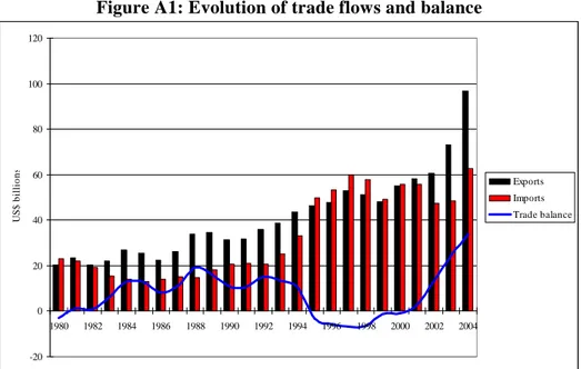
See Figure A1 in appendix, for the evolution of international trade flows and balance. 10

currency was devaluated by about 50% in nominal values. Though seeked results on exports and imports were not immediate, these measures managed to stop the trade deficit trajectory. From 2001 to 2004, trade surplus grew from US$ 2 billions to US$ 33 billions and by 2005 the Brazilian tariff had reached its lowest level with a simple average tariff of 11.1%.11

If we look at the sectoral structure of tariff protection throughout the 1987-2005 period we can see the magnitude of tariff cuts as well as the dispersion drop (see Figure 2). The largest tariff cuts concern the sectors with initially highest tariff levels, that is, manufacturing sectors such as automobiles, apparel and textiles. The lowest tariff cuts concern extractive sectors, with initially lowest levels. The levels of protection of agriculture and food sectors – where Brazil benefits from strong comparative advantage – are close to the Brazilian average tariff.12

<Figure 2>

Note that detailed information on non-tariff barriers (NTBs) is not available on a disaggregated basis to construct time-series across sectors in Brazil, and has not been included in this study. This should not be very problematic, from the moment that tariffs are the main policy instrument in Brazil. Though NTBs may have played a role as a trade barrier until 1990, since then they have become a relatively insignificant protectionist instrument.13

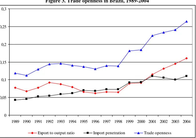
All these changes in trade protection together with those occurred in macroeconomic environment and policies affected trade performance in Brazil as a whole as well as in the different Brazilian states. Figure 3 shows the three usual indicators of international trade exposure – trade openness, import penetration and export to output ratios – for Brazil. Since 1989, trade openness has more than doubled, reaching 26.4% in 2004 (compared to 11.8% in

11

Several authors (Carvalho and DeNegri, 2000; Pourchet, 2003; Ribeiro, 2006) suggest that export volumes are becoming more sensible to the evolution of international demand than to exchange rate. In 2004, the real appreciation of the Brazilian currency (about 10% along the year) was not strong enough to reduce the positive effect of international demand on exports.

12

Though some interest groups representing the entrepreneurs might exert some influence on the trade policy making, in the case of Brazil it was limited to very specific sectors (see Abreu, 2004). Since Brazil committed to an economywide liberalization process and experienced the greatest tariff cuts in the most protected sectors, the question of the endogeneity of trade liberalization, that is sometimes raised when studying its impact on income distribution, should be less of an issue in the Brazilian case as already underlined by Goldberg and Pavcnik (2007).

13

Goldberg and Pavcnik (2007) emphasize that in recent years in developing countries, NTB coverage ratios and tariff rates (as well as their changes), whenever available, are positively correlated, indicating that they have been used as complements and not substitutes. In the case of Brazil, Carvalho (1992) considers that NTB’s application before 1990 was usually done in complement with high level tariffs causing a tariff redundancy and having no additional effects on imports. In 1997 the Brazilian government imposed some sanitary measures, but they did not seem to have played an efficient role in restricting imports.

1989 and 13.8 % in 1998).14 Changes were more important from 1998 onwards. The large increase in trade openness between 1998 and 2004 is mainly due to the growth of exports, with a rise of almost 10% of export exposure compared to around 4% for import penetration.

<Figure 3>

Given that our empirical framework studies the impact of openness to trade at the state level, a detailed description of trade exposure across Brazilian federative units is given in the next section, after the presentation of our different data sets.

3. Trade, poverty and inequality in Brazil: data and descriptive analysis

3.a. Data description

The data used in this study come from different sources. The first source is the household level micro-data from the Pesquisa Nacional por Amostra de Domicílios (PNAD), which is conducted annually by the Brazilian Census Bureau, the Instituto Brasileiro de Geografia e Estatística (IBGE).15 The survey, which samples about 300,000 individuals per year, is nationally representative and ensures coverage of both rural and urban areas of all states of the federation, except for the rural areas of the Northern Region, corresponding to the Amazon rainforest.16 From the PNAD we use individual level information to construct harmonized summary variables on income distribution, employment, education and various other socio-demographic characteristics (detailed below), at our unit of analysis, the state. When appropriate, we will make the distinction between rural and urban areas within states, for which all summary variables have in turn been constructed.17

14

Note that this level continues to be low compared to other Latin American countries partly because of the large size of Brazil.

15

During the period of analysis, there have been three years in which the PNAD was not carried out: in 1994 for budgetary reasons and in 1991 and 2000, because they were census years.

16

The rural areas not covered by the PNAD until 2003 and therefore excluded from our analysis, correspond specifically to the states of Acre, Amapá, Amazonas, Pará, Rondônia and Roraima, which, according to census data, represent about 2.3% of the Brazilian population. According to the PNAD surveys, in 1987 about 77 percent of the population was living in urban areas and in 2005 this share reached 86 percent, without the 6 states here cited.

17

The number of states considered in this study is twenty-six. Tocantins was created in 1988 as a dismemberment of Goiás state, but the distinction among the two states was not made in the PNAD before 1992. Due to the exclusion of rural areas in the Northern region before 2003, the number of cross-sectional units will be of twenty-six in urban areas and twenty in rural areas.

The definition of income used throughout the analysis corresponds to gross monthly household income per capita, measured in 2006 Brazilian Reais, and the sample considered is the total population.18 Various measures of inequality and poverty have been considered for the sake of robustness. In the case of inequality, we apply two well-known measures, the Gini and the Theil indices. When looking at poverty, again two standard poverty measures belonging to the Foster-Greer-Thorbecke (FGT) family are calculated: the headcount index and the poverty gap.19 The first one captures the proportion of the population living below the poverty line and the second one allows us to account for differences among households in the distance to the poverty line. The poverty line is here set at R$100 per person per month (in 2006 values), though robustness to the choice of threshold has been tested.20 In an effort to better gauge what is happening behind these summary statistics, we will also calculate income levels across quintiles (and deciles) of the income distribution and include them in our econometric study.

The PNAD provides us with information at the individual level that can be exploited for our econometric analysis. We are able to observe, among other things, the labor market status of individuals in the population, as well as the industrial sector in which they work.21 We are also able to observe a list of individual socio-demographic variables usually considered as determinants of income levels. From such individual-level data we construct different control variables, at the level of the state (or the rural/urban areas within states), in particular: the share of individuals in each state by years of schooling (grouped in six categories: none; 1 to 3 years; 4 to 7 years; 8 to 10 years; 11 to 14 years and 15 or more years) , the share of individuals in each “race” group (information on “race” is self-declared in the PNAD and distinguishes five groups: indigenous, white, black, Asian and mixed), the share of the

18

Monetary values are inflated to the September 2006 prices using the IBGE deflators derived from the INPC national consumer price index (see Corseuil and Foguel, 2002; Cogneau and Gignoux, 2009).

19

The general formula of the FGT family of poverty measures is:

∑

[

(

)

]

= − = q i i z y z n FGT 1 / 1 α α where z is the

poverty line, yi is the household’s per capita income level, n is the number of households, q is the number of poor households and α is a parameter determining the weight given to the distance of households to the poverty line. An α equal to zero gives us the headcount ratio and an α equal to one represents the poverty gap.

20

Though Brazil does not have an official poverty line, an ad-hoc administrative poverty line of about R$100, corresponding to the means-test in Brazil’s main new cash assistance program, Bolsa Familia, is gaining usage in the research community (see Ferreira et alii, 2006). As a robustness check, a poverty line of R$75 has also been tested.

21

Labor-market variables are available from the PNAD for individuals aged ten years or more. We will consider this population for all labor-market variables as well as for education variables in each state. The classification of industrial sectors used in this paper is given in Table A1 of the appendix.

agricultural sector22 in each state, the share of the informal workers, the share of workers by industrial sector.

In order to represent trade policy changes and openness to trade of Brazilian states, we use two different sets of measures. The first set comprises trade policy based measures, built on Brazilian nominal tariff data. The second set focuses on trade flows and reveals a state’s exposure to international trade, or its integration to world markets.

The data on trade policy are industry-specific nominal tariff rates. These are drawn from Kume et alii. (2003) for the 1987-1994 period. For the 1995-2005 years, data were made available by H. Kume. The tariff data series correspond to the nominal level of protection for 31 industry sectors.23 These data are a standard source on the Brazilian tariff structure.

Since we adopt a regional approach, we follow Topalova (2005) and construct an indicator to measure the influence of trade policy and its change at the state level in Brazil (and at the level of urban and rural areas within states). This indicator, called LIB, is a weighted average of national industry-level tariffs, where the weights correspond to the initial share of employment by industry within each state (the initial year in our study is 1987). It is computed as follows: 1987 1987 ) ( s k kt sk st L Tariff L LIB

∑

where s stands for the unit of analysis (the Brazilian states), k for the sector and t for time. Tariffkt refers to the tariff in the sector k for the year t, Lsk1987 to the workers employed in the

sector k for the year 1987 in the unit of analysis s and Ls1987 to the total workers in the unit of

analysis s for the year 1987.

The weights are calculated with data on employment for a year prior to trade reform, here 1987, ensuring that employment changes over time due to tariff variation are not included in

22

The share of agricultural sector takes into account the number of individuals that declare their industrial sector to be either agriculture or agri-food industries.

23

These 31 sector-specific ad-valorem tariff levels correspond to weighted averages of more disaggregated product-specific ad-valorem tariffs, where the weights are the value added in each narrowly defined product group.

our LIB measure of exposure to the tariff reforms. The data on employment by federative unit and industry in 1987 were drawn from the PNAD. Our use of household survey and tariff data with different industry definitions required a concordance between the two datasets. To match the data on tariffs (in the classification nivel 50) and employment (in the PNAD classification), we used the Table A1 of Industry Concordance (in the appendix) developed by Ferreira et alii. (2007a). As a result of this procedure, we are able to compute our trade liberalization indicator LIB for a group of 22 industries, in a sample of twenty-six states through the period 1987-2005.24

The data on trade flows is composed by the following indicators: import penetration (imports as a percentage of output plus net imports), export exposure (exports as a percentage of output) and trade openness (defined as the ratio of imports plus exports on gross domestic product). These ratios are calculated at the state-level and no urban-rural distinction within states is possible in this case. Trade data on imports and exports of federative units in current US dollars are collected by the Secretaria de comércio exterior (SECEX), Ministério do Desenvolvimento, Industria e Comércio Exterior (MDIC).25 The series on gross domestic product by state in current market prices come from the regional accounts of Brazil established by IBGE. These data were converted in current US dollars, using the annual average exchange rates.26 The trade flow indicators are calculated for total trade but also separately for the agricultural sector and the industrial sector (the latter including extractive and manufacturing industries) for the period 1989-2004.

3.b. Trade, poverty and inequality in Brazilian states

24

The original data provide the tariff levels for 31 sectors at the Nivel 50 industrial classification. We have aggregated the data by taking simple averages of reported tariffs (after verifying the high correlation of both series, unweighted and weighted by import penetration), so that the tariff information now matches the level of industry aggregation in the labor force data (22 industries).

25 _{These data series are only available since 1989 (seehttp://aliceweb.desenvolvimento.gov.br/default.asp). Note} that according to the SECEX, the state that exports is the one where agricultural products are cultivated, ores extracted and manufactured goods produced totally or partially. In this last case, the “exporting” state is the one that has completed the last step of the manufacturing process.

26

As the first years of our period of study were characterized by high inflation rates, the choice of the exchange rates matters. Therefore, robustness to this choice was tested through another method of calculation. Using states’s GDP series of the IBGE in current market prices, we have calculated the share of each state in the total Brazilian GDP. The GDP of each state was then calculated by applying these shares to Brazil’s GDP in current dollars from the database World Development Indicators (WDI, World Bank). The two methods give very similar values for the whole period under study.

Before estimating the distributional effects of international trade in Brazilian states, it is useful to show how heterogeneous are Brazilian states in terms of their exposure to trade and their poverty and inequality experiences.

A detailed picture of trade patterns by Brazilian federative units in 1989 and 2004 is given in Figure 4. Values observed show important spatial inequalities with a high level of trade exposure of some Brazilian states.27 If trade openness has increased in each state during the period under study, disparities between the different federative units have also grown: the “average” level of trade openness for the twenty-six states rose from 8% to 19.6% (standard deviations being 0.07 and 0.16 respectively). In 2004, trade openness ratios range from 0.9% in Acre (a state covered mostly by the jungle of the Amazon Rainforest) to 44.8% in Amazonas (whose main economic activities are concentrated in the free-export zone of Manaus) and 59.9% in Espírito Santo (a state with an extensive coastline that comprises some of the country’s main ports). Six additional Brazilian states reach openness ratios above 30%.28

<Figure 4>

Figure 4 also maps the separate levels of export exposure and import penetration ratios of Brazilian states, both in 1989 and 2004. Some Brazilian states exhibit a very important rise of export to output ratios during this period. In 1989, only five states reached an export exposure above 10%; in 2004 it is the case of twelve states, with four states above 25%: Espírito Santo and Pará - two states in which exports of iron ore play a major role -, Mato Grosso and Paraná, where soybean exports are very important. The evolutions are more modest for import penetration: in 1989, ratios are below 5% in all the Brazilian states except Amazonas, Rio de Janeiro, Espírito Santo and Rio Grande do Sul. In 2004, only eight states have ratios above 10%, with Amazonas and Espirito Santo showing levels above 25%. In line with what was observed for Brazil as a whole, it is mainly the growth of exports that accounts for the increase in trade openness in the different federative units.

27

Brazil is a very large country where trade policies but also distance, natural barriers to trade, transport infrastructure or access to major seaports play an important role concerning trade integration of the different federative units.

28

Mato Grosso (36.9%), Parana (36.1%), Para (34.8%), Maranhao (34.8%), Sao Paulo (31.2%) and Rio Grande do Sul (31.1%).

Note that an important feature of the Brazilian case is its strong geographical concentration of exports and imports. In 2004, three states29 represent more than 50% of total Brazilian exports while twenty states have a share in total exports below 5%. Geographical concentration of imports is even more important, even if it has fallen since 1989: while twenty one states have a share in total imports below 5% in 2004, three states30 represent more than 60% of total Brazilian imports.

From this analysis, it follows that integration to world markets was very uneven across the different federative units at the end of the eighties and that these regional inequalities in terms of trade exposure have increased during the last two decades. This variation across space and over time in trade patterns in Brazil might play a role on the different evolutions of state inequality and poverty levels.

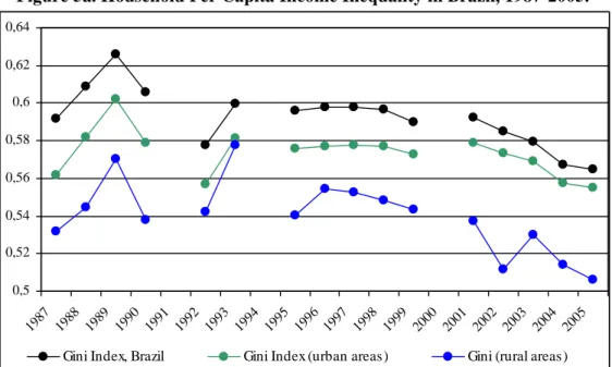
Figures 5a and 5b show respectively the evolution of two of the most common indicators of inequality and poverty, the Gini index and the headcount ratio. The trends are provided for Brazil as a whole as well as separately for rural and urban areas, over the period 1987 to 2005. The evolution of the Gini index reveals a steady increase of inequality from 1987 to 1989 (where a peak is reached at 0.63), followed by a certain degree of volatility until 1993. Usual explanations of such evolution include high and accelerating inflation over the period, as well as increasing education levels of the population, together with widening returns to schooling (see Ferreira and Paes de Barros, 2004). From 1993 to 2005 an initially slow but steady decline of inequality took place (from 0.60 in 1993, by 2005 the value of 0.56 was reached). Such decline was more intense in rural areas than in urban zones and particularly significant from 2001 onwards. When looking at poverty indicators over the same period we observe a similar pattern. The headcount ratio displays fluctuating values from 1987 to 1993, again reflecting macroeconomic instability and hyperinflation. From 1993 to 1995, a fall in the poverty headcount is observed. The introduction of the Organic Social Assistance law in 1993, which consisted essentially of unconditional cash transfers to poor old people living in rural areas and to the handicapped, together with the Real Plan in 1994, are usually cited among the relevant contributors to this initial poverty reduction (Ferreira et alii., 2006; Pero and Szerman, 2009). A period of relative stability in the percentage of poor at around 33%

29

Sao Paulo (35% in 1989 and 32.2% in 2004), Minas Gerais (respectively 13.7% and 10.4%) and Rio Grande do Sul (respectively 10.8% and 10.2%)

30

Sao Paulo (41% in 1989 and 43.1% in 2004), Rio de Janeiro (respectively 23.7% and 10.1%), Rio Grande do Sul (respectively 10.7% and 8.4%)

followed from 1995 until 2003 (though in rural areas poverty ratios continued a slow and steady decline). Finally, a persistent and significant fall in poverty ratios took place from 2003 onwards, this time both in urban and rural areas (the headcount index reaching 29% for Brazil in 2005).31

<Figures 5a and 5b>

Concerning the spatial dimension, when we look at the period of analysis 1987-2005, not only there are important differences in inequality and poverty between rural and urban areas, but also across Brazilian states, both in levels and in trends. Figure 6a and Figure 6b show the initial and final years’ measures of, respectively, Gini coefficients and headcount ratios in Brazilian states. Though inequality has fallen in almost all federative units32, the intensity of the drop varies across states. A similar spatial heterogeneity of experiences is observed when looking at poverty levels. In fact, no convergence across states seems to have taken place during the time frame of analysis.

<Figures 6a and 6b>

The aim of this paper is to investigate if the rich spatial variation in welfare outcomes and trends observed in Brazil is linked to the one observed in the degree of trade exposure of Brazilian states. Our estimation strategy and results are described in the next section.

4. Impact of trade liberalization on inequality and poverty

4.a. Econometric specification.

31 _{A few tentative explanations for these more recent declines in inequality and poverty levels in Brazil have} been put forward by the research community, among which: the observed declines in inequality between educational subgroups of population (due to a reduction in the educational heterogeneity of the labor force together with a compression in the distribution of returns to education), a better integration of rural and urban labor markets, a potential reduction of “racial” inequalities and the increase and better targeting of social transfers, with the adoption and expansion of conditional cash transfer programs (Ferreira et alii., 2006; Ferreira et alii, 2007b; Paes de Barros et alii., 2006).

32

The only exceptions are the two wealthy states of Distrito Federal and more importantly Sao Paulo, plus Rondonia, Acre, Roraima, Amapa –four states in the North of Brazil, a low-income cluster in the country for which only urban data are available .

To empirically estimate the effect of trade liberalization on inequality and poverty at the state level (or at the level of rural and urban areas within states), our main econometric specification is of the form:

st t s i ist i st st TradeLib X y =θ +

∑

where y denotes the level of inequality/poverty in state s at time period t. As described in _st the data subsection, different income distribution measures are used as our dependent variable: the Gini and the Theil indices to capture inequality and the headcount ratio and poverty gap indices to capture poverty levels.

In this study, TradeLibst is the key variable and we use two measures for it: a measure based

on trade policy (our indicator LIB described above) and indicators based on trade flows (lagged import penetration, lagged export exposure and lagged trade openness). All these indicators represent different ways of capturing the degree of trade exposure of Brazilian states. Hence, θ is the parameter of primary interest.

The vector Xist includes i control variables typically assumed to affect levels of poverty and

inequality. Our main specification includes as controls: the share of individuals declaring themselves as “white” in each state (to account for “racial” inequalities); the share of individuals by different levels of years of schooling in each state (to consider the role of educational inequalities), the share of the informal workers in each state and the size of the agricultural sector in each state (both well known determinants of the income distribution). Finally, λs and t are the state and time specific fixed effects respectively and εst is the error

term.

Based on regional data, this paper seeks to answer the question of the impact of trade liberalization on regional outcomes, or more precisely within states. An underlying assumption in this type of analysis is that labor should not be too mobile across states within Brazil at least in the short or medium run (there would be no differential effects throughout the country if wages, and consequently household income levels, were equalized across regions). However, as emphasized by Goldberg and Pavcnik (2007, p.56), “failure of this premise to hold in practice does not invalidate the approach; it simply implies that one would not find any differential trade policy effects across industries/regions in this case”. In the case

of Brazil, even though geographical migration is not negligible throughout the period of study, it is not sizeable enough to wipe off the spatial disparities in experiences observed.33

4.b. Empirical findings

4.b.i. Trade policy, poverty and inequality.

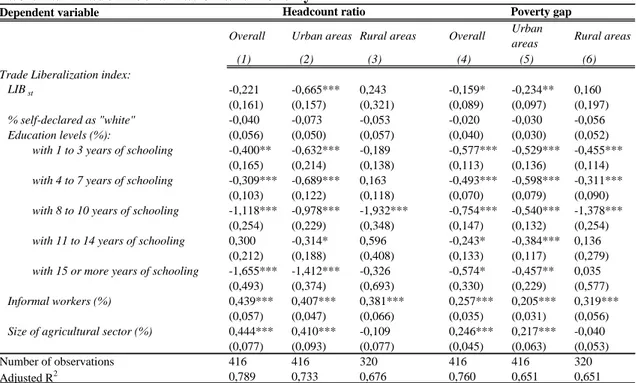
The estimated effects of our trade policy indicator LIB on poverty are presented in Table 1a. The table reports equation (1) estimated using both the headcount ratio and the poverty gap index as poverty indicators. For each dependent variable, results are reported using the state as a whole as unit of analysis (columns 1 and 4), but since rural and urban areas within states may be very different, we also examine equation (1) separately for urban areas (columns 2 and 5) and rural areas (columns 3 and 6) within states.

Table 1a shows a negative effect of our trade policy indicator LIB on poverty when we look at the state level (columns 1 and 4), though only statistically significant when poverty is measured by the poverty gap (and only significant at 10%). This means that, at the state level, trade liberalization might contribute to poverty increases. In other words, even if over the period studied Brazilian states experienced in general a fall in poverty, Brazilian states that were more affected by tariff reductions experienced smaller reductions in poverty (at least in terms of the poverty gap index). Our estimation suggests that, on average a fall of one percentage point in the trade policy indicator LIB would lead to an increase in the poverty gap of 0.16 percentage point.

The fact that rural and urban areas within states are very different may be behind our low significance levels when the state as a whole is used as unit of analysis. In fact, if we concentrate on urban areas only (columns 2 and 5), the negative effect of trade liberalization on poverty is highly significant and the size of coefficients on our trade policy indicator LIB is

33

To get insight of geographical migration in Brazil, we use PNAD surveys: since 1992, the percentage of individuals that declare themselves living in the same state for the past 10 years is close to 90%. Only about 5% declare themselves as being living in their state during less than 4 years. These percentages are obtained considering the total population. Other studies, such as for example Fiess and Verner (2003) find a much larger percentage of migrants (they present numbers that go up to 40%). However they only focus on household heads (and not total population), and they classify them as migrants from the moment that they have migrated at least once during their entire lifetime. Indeed in a footnote they indicate that their methodology overestimates migration numbers, with respect to what the Brazilian Census data show.

also larger, no matter which poverty measure is used. On average a fall of one percentage point in the trade policy indicator LIB in urban areas of states would lead to an increase in the headcount ratio of 0.67 percentage point, and an increase in the poverty gap of 0.23 percentage point. On the other side, no significant effect is observed in rural areas (columns 3 and 6).

In the estimation of equation (1) we included a few control variables that are considered to be usual determinants of poverty and inequality. Concerning our poverty results in Table 1a, controls are almost all highly significant and have the expected signs. Education is almost always significant and lowers poverty at practically all levels of education, while an increase in the share of informal workers leads to a significant rise in poverty. The size of the agricultural sector in a state matters: it leads to a significant rise in poverty.34 As expected, informal jobs and agricultural employment show up as significant determinants of poverty. The share of individuals declaring themselves as “white” is never significant.

<Tables 1a and 1b>

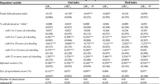
Table 1b documents the relationship between trade liberalization and inequality. When we consider the state as a whole as unit of analysis (columns 1 and 4), our trade policy indicator is inequality increasing, but the effect is only significant using the Theil index. In other words, Brazilian states that were more affected by tariff cuts experienced smaller reductions in inequality (at least in terms of the Theil index). However, opposing and significant patterns emerge when we consider urban and rural areas separately, these patterns being robust to the choice of inequality measure. The influence of a tariff reduction is inequality increasing in urban areas (columns 2 and 5) and inequality decreasing in rural zones (columns 3 and 6).35

34

Our variable capturing the size of the agricultural sector is not significant in rural areas, where almost all economic activity concerns agriculture. In any case, our results on the variable of interest LIB are robust to the omission of this variable.

35

Note that the relationship between control variables and inequality is less straightforward than in the case of poverty. In particular, the interpretation of schooling levels is not easy. When we look at the distribution of the population among different levels of schooling, the only category for which we obtain a consistent and significant coefficient, concerns the most educated. The share of adults with more than 15 years of schooling (or more than 10 years in rural areas) unequivocally has a positive and significant effect on inequality (such individuals are eventually those at the highest end of the income distribution). An increase in the share of informal workers in a state leads to a rise in inequality, except for rural areas where no significant effect is found. Finally, other control variables (the share of individuals declaring themselves as “white” or the size of the agricultural sector) are insignificant or not robust to the choice of inequality measure.

One tentative explanation for our contrasting effects of trade liberalization on household poverty and inequality between urban and rural areas could be that urban workers – essentially employed in the manufacturing industries and in the service sector – suffered the most from the liberalization process. Previous research on Brazil has established that trade liberalization led to a decline in economy-wide wage inequality (Gonzaga et alii, 2006; Ferreira et alii, 2007a). At the same time, recent evidence on labor reallocations in response to trade reforms shows labor displacements from import competing industries, but neither comparative-advantage industries nor exporters seem to have absorbed trade-displaced workers for years. Indeed, more frequent transitions to informal work status and unemployment are observed (Menezes and Muendler, 2007). These transitions may be sources of poverty and inequality increases and these effects are captured when total household income (and not only wages) is considered. If these adjustments played a relatively more important role in urban areas than other inequality decreasing mechanisms, they may be behind our poverty and inequality increasing results in urban areas, and may also help explain the differences between rural and urban results. Though it is beyond the scope of this paper, our results suggest that a better understanding of the effects of trade liberalization on household income distribution should take into account not only the observed changes in labor income, but also if trade-induced changes in household composition and occupational situation of all household members have occurred.36

Note also that trade liberalization was more intense in manufacturing sectors, with major tariff reductions taking place from 1990 onwards (see section 2). For agricultural sectors, the reduction in protection was less important from 1990 onwards and Brazil has strong comparative advantages in these sectors, where an important rise in exports has occurred (see subsection 4.b.ii).37 So when only rural areas within states are considered, it is not surprising

36

To our knowledge, the only study that has tempted to investigate the implications for household income distribution of trade-driven changes in wages is Ferreira et alii (2007a). Using earnings-based simulations and looking at Brazil as a whole, they observe that reductions in wage inequality appear to extend to declines in household income poverty and inequality. However, as the authors recognize, their “earnings-based simulations are not the most suitable way for understanding differences between full household income distributions” (p.31), as the indirect impacts of trade on family composition or on occupational decisions of household members other than the spouses are not considered. Though our framework of analysis is not comparable, since our units of analysis are Brazilian states and not Brazil as a whole, our differential results across urban and rural areas should encourage additional research on the various trade-transmission channels that operate for household income distributions. Ferreira et alii (2007a) point, for example, to the use of more general specifications of micro-simulation models (Bourguignon et alii, 2004) to study the welfare impacts of trade reforms.

37

The average tariff for agricultural products remained under 10% since 1989 whereas the average tariff for all products still exceeded 30% in 1989 and remained since then above 10%.

to find no significant effects in terms of poverty from trade liberalization and to even have levels of inequality reduced if anything.

Another reason for observed differences in results on poverty and inequality across urban and rural areas may be related to a differential role of social transfers. In particular, due to the major role of conditional cash transfer programs in poverty reduction, we were concerned that if these transfers were correlated with exposure to trade, their omission would result in omitted variable bias. Unfortunately with our data we cannot identify the sources of income of individuals (and more specifically transfers received) for the whole period of analysis nor can we capture federal expenditures by state.38 But we know that conditional cash transfer programs were initially implemented in a few municipalities, to be then launched nationwide in 2001 (essentially with the introduction of Bolsa Escola and Bolsa Alimentação programs, then unified and amplified in the Bolsa Familia program in 2003). We decided to re-run our regressions excluding the period 2001-2005 and our results are still robust. Though the size of our coefficient on trade liberalization falls in poverty and inequality regressions by around 30% on average, we still observe opposing and significant effects across urban and rural areas within states.

To sum up, our results show that trade liberalization, measured by our indicator LIB, increases poverty and inequality in Brazilian states, though these effects are mildly significant. The distinction between rural and urban areas gives more insight on the effect of trade liberalization. In urban areas we observe a negative and always significant effect for both poverty and inequality. In rural zones, the sign of the effect of trade liberalization is reversed (though significant only when looking at inequality). Our findings on state poverty are in line with recent results for Indian districts (Topalova, 2005), even though no parallel significant effect on inequality is found in India. Note that the poverty increase due to trade liberalization observed in India takes place in the rural world, while in Brazil it appears to occur in urban areas. While, in the case of India, sectors that have been relatively more affected by tariff reductions are concentrated in rural districts, descriptive evidence for Brazil (Figure 2) shows

38

We could only construct series of local social security and social assistance expenditures made by states. But these variables only capture a minimal part of public transfers received by households and proved irrelevant. Besides, the role that the establishment of rural pensions may have played in rural areas cannot be taken into account, because PNAD surveys do not allow us to identify these sources of income for the whole period of analysis.

that trade liberalization was more intense in manufacturing sectors, typically implanted on urban zones.

We have investigated whether these results are robust to the choice of the indicator on trade liberalization. In our trade policy measure LIB, tariffs are weighted by the number of workers in each industry as a share of total employment in each state. Some authors (Topalova, 2005; Edmonds et alii, 2007) raised the question of considering employment only in “tariff-protected” industries. Therefore, an alternative indicator LIB2 is also constructed where the employment shares are calculated over employment only in “tariff-protected” industries, that is: ) ( ) ( 2 1987 1987

∑

∑

where s stands for the unit of analysis, k for the sector and t for time.

A problem with LIB2 is that it does not reflect the size of the traded sector within a state. Consider two states with the same structure of employment in “tariff-protected” industries; the indicator will now have by construction the same value across the two states even if shares of workers in “tariff-protected” industries on total employment are very different. As a consequence, the magnitude of trade policy effects may be overstated by construction with LIB2. To overcome this problem another estimation strategy, instrumenting LIB by LIB2, is implemented. In both cases we obtain similar effects of trade policy on our income distribution variables at the state level: when significant, the effect of trade liberalization is poverty and inequality increasing (see tables A2 and A3 in the appendix).

Additional robustness checks have been performed. In particular, we estimated regressions without states that can be considered as outliers, like Distrito Federal and Amazonas. On one hand, Distrito Federal (Brasília) has a very peculiar productive, labor and revenue pattern from the rest of the country as it is a fundamentally administrative city which concentrates the major part of national government activities. Amazonas, on the other hand, benefits from special trade regimes because of the status of “free trade zone” detained by the Manaus industrial area. Regarding poverty, a different poverty line of R$75 was also tested. In all cases our main results hold.39

39

4.b.ii. International trade, poverty and inequality

Brazil is one of the few countries where international trade flows can be observed and measured by federative units, and where the number of units of analysis allows the use of a regression framework to study the effects on state poverty and inequality of trade openness, import penetration and export exposure. These indicators reflect the degree of integration of Brazilian states to world markets. Note that they differ from our LIB measure based on tariffs cuts. They are not exclusively influenced by trade policies, as trade flows are also determined by other factors such as transport costs, macroeconomic measures, factor endowments, the country’s size and geographical situation, etc. Our dataset allows us to distinguish between the effects of imports and exports on poverty and inequality. The responses of poverty and inequality indices to our trade flows based measures are documented in tables 2a and 2b respectively. Because it is not possible to have data on trade flows separately for rural and urban areas within states, we only provide evidence using the state as a whole as unit of analysis. However, in an effort to study the influence of trade integration on poverty and inequality at a more disaggregated level, we have constructed import and export ratios separately for agricultural and industrial sectors. These results are shown in Table 3.

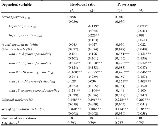
Table 2a presents the results on poverty incidence (columns 1 and 2) and poverty depth (columns 3 and 4). For each poverty measure, two specifications are tested to capture the effect of international trade: (i) the inclusion of a measure of lagged trade openness (defined as the ratio of imports plus exports on gross domestic product) and (ii) the inclusion of lagged import penetration and lagged export exposure ratios simultaneously. A similar specification structure is followed in Table 2b to capture the impact of international trade on both Gini and Theil inequality measures.

<Tables 2a and 2b>

Two noteworthy results emerge. First, for both poverty and inequality, trade openness has no significant impact, no matter which income distribution measure is used (see coefficient on the variable Trade opennesss(t-1) in columns 1 and 3 of both Tables 2a and 2b). However, a

different picture emerges from the moment we dig into the separate influence of export exposure and import penetration (see coefficients on the variables Export exposures(t-1) and

exposure appears to have reduced poverty and inequality quite significantly while the growth of import penetration has increased both income distribution measures. If we evaluate the magnitude of coefficients, from column 2 in Table 2a we see that a rise of one percentage point in import penetration experienced in a state would lead to an increase in poverty incidence of 0.23 percentage point (significance is lost for our poverty depth measure in column 4). For export exposure, a percentage point rise would, on the contrary, lead to a fall in poverty of -0.12 using the headcount ratio (-0.07 with the poverty gap). Concerning inequality, a rise of one percentage point in import penetration increases the Gini coefficient of 0.12 percentage point (0.34 for the Theil index), while a percentage point rise in export exposure would lead to a variation in the Gini coefficient of -0.11 percentage point (-0.33 in the Theil index).

To sum up, we see that import penetration yields results that are consistent with our findings obtained with the trade policy based measure: a rise in the import penetration ratio increases poverty incidence and inequality at the state level. At the same time, tariff cuts -when significant- were also related, at the state level, to rising poverty and inequality levels On the contrary, trade integration through rising export ratios clearly contributes to a fall in poverty and inequality.

In Brazil, agricultural exports have experienced a rapid growth (551% between 1989 and 2004 in current dollars), much larger than the increase of industrial exports (168% on the same period). On the other side, agricultural imports have grown less than industrial imports (36% against 268%).40 Concerning trade intensity, export exposure and import penetration ratios are in 2004 considerably stronger for industry (the state’s average export exposure ratios for industry and agriculture were respectively 32.4 and 8.5 in 2004; in turn, the state’s average import penetration ratios reached 37.9 and 22.8). To see if differential effects on income distribution measures appear according to the sector concerned, Table 3 presents the effects of international trade on poverty (columns 1 and 2) and inequality (columns 3 and 4) when export and import ratios are constructed separately for the agricultural and the industrial sectors (the latter including extractive industries).

<Table 3>

40

Our results show, once more, an opposite sign for export exposure and import penetration effects on welfare both for industry and agriculture. In the industrial sector as well as in the agricultural sector, export exposure has reduced poverty and inequality while import penetration (when significant) has increased both welfare measures. In sum, no clear differential effect is observed between the industrial and agricultural sectors in terms of the impact of trade exposure on poverty and inequality.

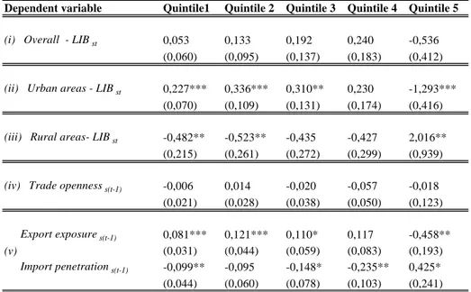
4.b.iii. The effect of trade exposure on income distribution: quintile analysis

When summary inequality measures such as the Gini or the Theil index are used, we cannot easily tell where about in the income distribution variations are taking place. In an effort to better seize how trade liberalization affects the shape of the entire income distribution in each state, instead of just focusing on summary statistics of poverty and inequality, we have also estimated income levels for each quintile (and also by decile) in each state s at time t, and run the additional set of equations:

st t s i ist i st stj TradeLib X y =θ +

∑

Where y_stj denotes the relative income level of the j-th quintile (or decile) normalized by the mean, in state s at time period t.

<Table 4>

Table 4 presents a summary of all our estimations of equation (2) for each quintile41. For the sake of simplicity, only the values and standard errors of the coefficients on our variables of interest are reported, that is: (i) on our trade policy indicator LIB using the whole state as unit of analysis; (ii) then considering only urban areas within states; (iii) and only rural areas within states; (iv) on our indicator of lagged trade openness; (v) and finally on our measures of lagged import penetration and export exposure ratios simultaneously included in the regression.

41

Complete quintile regressions are available from the authors upon request. Decile regressions leading to similar results were as well estimated and are also available.

Though no significant effect is found for trade policy measure LIB at the state level, no matter which quintile regression is considered, there is evidence of growing (falling) inequality in urban (rural) areas linked to trade liberalization: this comes from coefficients sharing a similar positive (negative) sign in all quintiles except the highest one, where the sign is reversed. Distributional changes due to trade liberalization are therefore observed along the income ladder (and particularly significant for the first, second and fifth quintiles). Concerning our trade flows based variables, the quintile regressions reveal again no significant effect of trade openness. However export exposure increases the relative income levels of all quintiles except the last one that presents the opposite sign, while import penetration increases the relative income levels of the upper quintile and decreases the relative income levels of the others quintiles (these effects being significant for almost all quintile levels). An interesting fact in Table 4 comes from the inspection of coefficient sizes by quintile. Independently of the variable chosen to measure trade exposure and of the levels of disaggregation in state population (state as a whole, urban or rural areas within states), the impact on relative income levels of quintiles is non-monotonic. Coefficients of the second quintile group are systematically larger than those of the first quintile counterpart, but not necessarily lower than those of the third or fourth quintile. In a sense, the effects of exposure to trade, though fully shared across the whole income ladder, seem relatively less strong among the poorest of the poor and middle quintile groups. The fact that the poorest of the poor are less affected then those households closer to the poverty line can be seen as hinted by results on our two poverty measures in previous regressions. When looking at the effects of our trade liberalization variables on both poverty incidence and poverty depth (Table 1a), coefficients are systematically lower in the second case (last three columns versus first three columns), when distance to the poverty line is taken into account.

5. Conclusion

Brazil has undergone an extensive trade liberalization reform since 1988 that has changed significantly the level of protection of the Brazilian economy. Since the nineties, Brazil has also experienced a slow but significant decline in both poverty and inequality indicators, though high levels of inequality and persistent poverty remain, with important geographical differences. Can we establish a causal link between changes in trade policies and international