The Impact of migration on rural poverty and inequality: a case study in China

Texte intégral

(1)2014s-08. The Impact of migration on rural poverty and inequality: a case study in China Nong Zhu, Xubei Luo. Série Scientifique Scientific Series. Montréal Janvier/January 2014. © 2014 Nong Zhu. Xubei Luo. Tous droits réservés. All rights reserved. Reproduction partielle permise avec citation du document source, incluant la notice ©. Short sections may be quoted without explicit permission, if full credit, including © notice, is given to the source..

(2) CIRANO Le CIRANO est un organisme sans but lucratif constitué en vertu de la Loi des compagnies du Québec. Le financement de son infrastructure et de ses activités de recherche provient des cotisations de ses organisations-membres, d’une subvention d’infrastructure du Ministère de l'Enseignement supérieur, de la Recherche, de la Science et de la Technologie, de même que des subventions et mandats obtenus par ses équipes de recherche. CIRANO is a private non-profit organization incorporated under the Québec Companies Act. Its infrastructure and research activities are funded through fees paid by member organizations, an infrastructure grant from the Ministère de l'Enseignement supérieur, de la Recherche, de la Science et de la Technologie, and grants and research mandates obtained by its research teams. Les partenaires du CIRANO Partenaire majeur Ministère de l'Enseignement supérieur, de la Recherche, de la Science et de la Technologie Partenaires corporatifs Autorité des marchés financiers Banque de développement du Canada Banque du Canada Banque Laurentienne du Canada Banque Nationale du Canada Banque Scotia Bell Canada BMO Groupe financier Caisse de dépôt et placement du Québec Fédération des caisses Desjardins du Québec Financière Sun Life, Québec Gaz Métro Hydro-Québec Industrie Canada Investissements PSP Ministère des Finances et de l’Économie Power Corporation du Canada Rio Tinto Alcan State Street Global Advisors Transat A.T. Ville de Montréal Partenaires universitaires École Polytechnique de Montréal École de technologie supérieure (ÉTS) HEC Montréal Institut national de la recherche scientifique (INRS) McGill University Université Concordia Université de Montréal Université de Sherbrooke Université du Québec Université du Québec à Montréal Université Laval Le CIRANO collabore avec de nombreux centres et chaires de recherche universitaires dont on peut consulter la liste sur son site web. Les cahiers de la série scientifique (CS) visent à rendre accessibles des résultats de recherche effectuée au CIRANO afin de susciter échanges et commentaires. Ces cahiers sont écrits dans le style des publications scientifiques. Les idées et les opinions émises sont sous l’unique responsabilité des auteurs et ne représentent pas nécessairement les positions du CIRANO ou de ses partenaires. This paper presents research carried out at CIRANO and aims at encouraging discussion and comment. The observations and viewpoints expressed are the sole responsibility of the authors. They do not necessarily represent positions of CIRANO or its partners.. ISSN 2292-0838 (en ligne). Partenaire financier.

(3) The Impact of migration on rural poverty and inequality: a case study in China * Nong Zhu †, Xubei Luo‡,. Résumé/abstract Large numbers of agricultural labor moved from the countryside to cities after the economic reforms in China. Migration and remittances play an important role in transforming the structure of rural household income. This paper examines the impact of rural-to-urban migration on rural poverty and inequality in a mountainous area of Hubei province using the data of a 2002 household survey. Since migration income is a potential substitute of farm income, we present counterfactual scenarios of what rural income, poverty, and inequality would have been in the absence of migration. Our results show that, by providing alternatives to households with lower marginal labor productivity in agriculture, migration leads to an increase in rural income. In contrast to many studies that suggest the increasing share of nonfarm income in total income widens inequality, this paper offers support for the hypothesis that migration tends to have egalitarian effects on rural income for three reasons: (i) migration is rational self-selection – farmers with higher expected return in agricultural activities and/or in local non-farm activities choose to remain in countryside while those with higher expected return in urban non-farm sectors migrate; (ii) households facing binding constraints of land shortage are more likely to migrate; (iii) poorer households benefit disproportionately from migration. Mots clés : Migration, poverty, inequality, China. Codes JEL : D63, O15, Q12. *. This article was published in Agricultural Economics, vol. 41, no. 2, p. 191-204, and won the award for The 2010 best paper in Agricultural Economics. † INRS-UCS, University of Quebec. Corresponding author: INRS-UCS, 385 rue Sherbrooke Est, Montreal, QC, H2X 1E3, Canada. Tel: 1-514-499-8281. Fax.: 1-514-499-4065. Nong.Zhu@UCS.INRS.Ca ‡ Senior economist, The World Bank, East Asia and Pacific Region, Poverty Reduction and Economic Management Department, cgoh@worldbank.org.

(4) 1 Introduction Rural-to-urban migration plays an increasingly important role in sustainable development and poverty reduction in rural areas (FAO, 1998; OECD, 2005; The World Bank, 2007). In many developing countries, non-farm activity, of which migration consists of an important part, often accounts for as much as 50% of rural employment and a similar percentage share of household income (Lanjouw, 1999a). In average, the ratio of non-farm income to total rural household income is about 42% in Africa, 40% in Latin America and 32% in Asia (The World Bank, 2000). In China, rural-to-urban migration and development of the rural non-farm sector strongly modified rural household income structure. Non-farm activities gradually became an important source for rural household income. In 2004, non-farm income reached 46% of the total rural income (National Statistics Bureau of China, 2005). Shortage of arable land is a binding constraint of agricultural productivity in China. Per capita farm income has always been low due to the limited marginal labor productivity. Conflicts between shortage of land and surplus of labor are more serious in poor areas. Peasants have a strong incentive to leave land for better job opportunities. The economic reforms, in particular the implementation of the Household Responsibility System (HRS), in the late 1970s not only stimulated the incentive of farmers and contributed to the sharp increase of agricultural productivity, but also legitimized rural redundant labor to leave land (litu) and countryside (lixiang). Since then, rural non-farm sectors and urban sectors have played an increasingly important role in absorbing surplus agricultural labor, enhancing rural income and reducing rural poverty. In only 21 years (1980-2001), the incidence of rural poverty fell from 76% to 13%, and rural income Gini increased from 0.25 to 0.37 (Ravallion and Chen, 2004; Ravallion, 2005). Whether the decline in poverty was principally due to farm income growth or due to non-farm 1.

(5) income growth and whether the rising share of non-farm income in total rural household income was the leading cause of the sharp increase in rural inequality have been key issues of debate. Some studies suggest that the rise in rural inequality in China since the beginning of the economic reforms has been largely due to an increase of non-farm income in total income for the following reasons: (i) distribution of non-farm income is more unequal than that of farm income; (ii) richer households have higher chances to participate in migration and local non-farm activities; and (iii) households with higher income are characterized by a higher participation rate in non-farm activities and a higher share of non-farm income in total income (see for example, Bhalla, 1990; Zhu, 1991; Knight and Song, 1993; Hussain et al., 1994; Yao, 1999; Wan, 2004; Wan and Zhou, 2005; Liu, 2006). Using data from a survey of rural households in Hubei province, we examine impacts of ruralto-urban migration on rural poverty and inequality. Taking into account of household nonobservable characteristics, we consider migration income as a “potential substitute” for household earnings, and simulate the counterfactual of how rural household income, rural poverty and rural inequality would have been in the absence of migration. Our results show that: (i) migration is selective across households, good farmers remain in local agricultural production; (ii) migration largely increases rural household income and reduces poverty; (iii) migration also reduces rural inequality as it benefits poorer households disproportionately . This paper is structured as follows. Section 2 studies economic reforms and rural labor mobility in China from a historical perspective. Section 3 reviews the literature on migration and income distribution. Section 4 presents the empirical analysis. Section 5 describes the data. Section 6 specifies the participation and income equations. Section 7 presents the results, and section 8 concludes.. 2.

(6) 2 Economic reforms and rural labor mobility Economic autarky and traditional agriculture have been characterizing the Chinese countryside for a long time. Following the model of the former USSR, China gave priority to the development of heavy industry at an early stage of industrialization. Farmers were heavily taxed; a large amount of agricultural surplus was transferred to industrial investments. The real income of farmers was hence artificially lowered due to the socialist price system, which over-priced manufactured products to raise profitability in industry while squeezed agriculture through the “price scissors” (Carr and Davies, 1971; Naughton, 1999). Before the reforms, in order to stabilize agricultural production, farmers were tied to the land in two ways: (i) through rural collectivization and (ii) through the civil status system called “hukou” (Davin, 1999). Rural collectivization tightened the links between farmers’ income and their daily work-participation in collective agriculture: a farmer earned “working-points” proportionately to the time spent on the collective land (McMillan et al., 1989). The civil status system consisted in codifying the supply of consumption goods and the access to jobs. Without acquiring the urban civil status, rural-tourban migrants could not settle on a permanent basis outside their place of origin. Before the reforms, these two rules divided Chinese society into two sharply contrasted segments: urban areas with a lower incidence of poverty and rural areas with high poverty. The economic reforms that began in the late 1970s brought huge changes to rural areas. First, the collapse of the system of “People’s Communes”, as well as the implementation and generalization of the Household Responsibility System (HRS), gave greater freedom to farmers: they could freely allocate their time and choose their income strategies and productive activities (Zhu and Jiang, 1993; de Beer and Rocca, 1997). By simply de-collectivizing production and allowing farmers to sell their surplus produce on the market, rural per capita income about tripled 3.

(7) in 1978-1984 (Zhang and Wan, 2006). Second, the agricultural reforms strongly increased agricultural production and the supply of grains in markets, which enabled people living in urban areas without the urban civil status to purchase food in free markets. It finally resulted in abandoning the rationing system. Since 1984, gradually, food market became open and housing in cities became marketable. These two factors enabled farmers to enter cities and stay there on a permanent basis without changing their civil status. Third, with the development of various nonstate enterprises, the urban labor market was gradually established, making it possible for ruralto-urban migrants to find jobs and to earn their living in cities. In addition, the development of urban infrastructure required extra labor for construction and the diversification of consumption resulting from the improvement of living standards created niches for a multiplicity of thriving small businesses. All these factors contributed to an increase in the demand for labor in urban areas, which resulted in a vast movement of agricultural labor from rural areas to cities (Banister and Taylor, 1990; Aubert, 1995). Although the segmentation of rural-urban labor market has been much improved after the economic reforms, the misallocation of labour resources still leads to a significant economic welfare loss. A recent study of the World Bank estimates the large potential gains from a greater labor market integration – using 2001 as a baseline, with a mere 1% labor relocation from rural areas to urban areas, the overall economy will gain by 0.5%. If the share of labor outflow reaches to 5% and 10%, the GDP will grow by 2.5% and 5%, respectively (The World Bank, 2005). Rural-to-urban migration deeply transformed the structure of household incomes in rural China. Remittances gradually became an importance source of income for rural households and served as an engine of growth for rural areas (de Braud and Giles, 2008). Rural-to-urban migration influences the rural economy through various channels. First, migration reduces the pressure on the demand for land in poor rural areas and contributes to breaking up the vicious 4.

(8) cycle of “poverty – extensive cultivation – ecological deterioration – poverty”. Second, remittances significantly increase total household incomes and hence enhance the investment capacity in local production. It can also mitigate income fluctuations and enable the adoption of some more profitable but “risky” agricultural technologies, which favors the transformation of traditional agriculture to modern agriculture (Islam, 1997; Bright et al. 2000). Third, remittances and other non-farm income are often a source of savings, which is of importance in food security. Households that diversify their income source by sending their members to outside labor market are less vulnerable to negative shocks.. 3 Migration and income distribution in sending communities Rural-to-urban migration undoubtedly increases rural income level in sending areas (Adams and Page, 2003; Straubhaar and Vadean, 2005). However, as to its impacts on income distribution, results are mixed. According to some studies, the dynamics of migration and income distribution might be non-linear (Stark et al., 1986; 1988; Jones, 1998; McKenzie, 2005; McKenzie and Rapoport, 2007). Remittance is an important component of rural non-farm income. Some studies show that the distribution of non-farm income is more unequal than that of farm income. As participation in non-farm activities is highly selective, non-farm income tends to increase income disparities, particularly in poorer areas.1 Some other studies, however, show that non-farm income can reduce inequality as it accrues disproportionately to poorer households, and its equalizing. 1. See for instance Adams (1998), Rodriguez (1998), Shand (1987), Reardon and Taylor (1996), Barham and Boucher. (1998), Leones and Feldman (1998), Elbers and Lanjouw (2001), Escobal (2001), Khan and Riskin (2001).. 5.

(9) impact becomes more important as the proportion of non-farm income in total income increases.2 There is a rich literature on rural poverty and inequality in China based on different datasets. Most studies have shown that, since the beginning of the economic reforms, aggregate household income has significantly increased and inequality noticeably widened (Kanbur and Zhang, 1999; Chen and Wang, 2001; Khan and Riskin, 2001; Wade, 2004; Liu, 2006; Chotikapanich et al., 2007). According to the research by the Ministry of Agriculture of China, income gap has widened, the Gini index increased from 0.3-0.4 in 1980s to over 0.4 since 1996 (Rural Economic Research Center, Ministry of Agriculture of China, 2003). Some studies suggest that the process of diversification into non-agricultural activities in rural areas tends to increase disparities, unlike the agriculture-based growth in the early 1980s, which equalized allocation of land kept income gaps at bay (Wan, 2004; Zhang and Wan, 2006). The more unequal distribution of non-farm income is a key factor explaining the rise in inequality in household income at the early stage of the reforms. Their conclusion implies that, with the continuing transfer of rural workers to nonfarm sectors in both urban and rural areas, income inequality in rural areas will continue to worsen (Bhalla, 1990; Hussain et al., 1994; Yao, 1999; Zhu, 1991). In our opinion, some existing research on income distribution in rural China has a certain limits. First, most of these studies correspond to meso-economic analyses using provincial or county level data. Income is usually measured as an average at the meso level, such as regional per capita GDP or income. However, farmers’ income distribution should be examined at the micro-level, as difference in income distribution may be the dominated difference in regional. 2. See for instance Chinn (1979), Stark et al. (1986), Taylor (1992; 1999), Adams (1994; 1999), Adams and He (1995),. Ahlburg (1996), Taylor and Wyatt (1996); Lachaud (1999), de Janvry and Sadoulet (2001), de Brauw and Giles (2008).. 6.

(10) characteristics when using meso data. Second, quite a few surveys show that households with higher income are usually the ones who work in the non-farm sector or run a business. However, we cannot conclude that households with higher income are more likely to participate in nonfarm activity and that development of non-farm sector will widen income gaps. Poor and rich households may both be inclined to participate in non-farm activities because the former have a stronger motivation whereas the latter have greater capability. The relatively poor households usually choose to engage in non-farm activities characterized by a higher labor-capital ratio and a lower financial entry barrier (FAO, 1998). Therefore, compared with households with better farm production conditions, households with lower income may choose to participle in migration and operate non-farm activities, which tends to narrow the income gap and lead to a more equal income distribution. In the literature, two methods are used to study the impacts of migration on inequality. One considers remittances as an “exogenous transfer” (Pyatt et al., 1980; Stark, 1991; Adams, 1994), and the other considers remittances as a “potential substitute” for home earnings (Adams, 1989; Barham and Boucher, 1998). The first method provides a direct and simple measure of how remittances contribute to total income by decomposing total household income and studying the distribution of each income source and its contribution to total income inequality. As remittances are taken as an exogenous transfer, which adds to the pre-existing home earnings, they are treated independently from home earnings. In other words, for a given household, with a given level of home earnings, an increase in remittances raises total income by the same amount. This could be true if the migration participation was to compensate a short term shock, such as a bad harvest or drought/flood. But, more often than not, participation in migration is a long-term alternative choice of participation in farm activity for households – migrants would contribute to their families in other ways if they had not migrated. Hence, this method does not address the 7.

(11) interdependence of migration and home production. The results are hence biased if there is substitutability between the participation in migration and home productive activities (Kimhi, 1994; Escobal, 2001). The second method compares the observed income distribution with a counterfactual scenario in the absence of migration and remittances by including an imputation for home earnings of erstwhile migrants. Taking into account the substitutability of migration and home productive activities, Adams (1989) estimates a function of household income determination for non-migrant households, and applies the coefficients and the endowment bundles of migrant households (in the absence of migration and remittances) to impute their earnings under a non-migration scenario to study the impacts of remittance on inequality. Barham and Boucher (1998) correct the selection bias and improve the income simulation model. Using a bivariate probit model of double selection, Lachaud (1999) moves a step forward to simulate household income obtained in the absence of remittance and migration, and examines the impacts of private transfers on poverty. In the following sections, we take into account interactions between the participation in various productive activities and analyze the impacts of migration on poverty and inequality using data from a rural household survey in Hubei province in China. We relax the assumption of the independence of migration and home production, and compare the observed household income distribution with a counterfactual income distribution in the absence of migration and remittances to identify the impacts of migration on inequality and poverty. Barham and Boucher (1998) imputed migrants’ home earnings using an income equation estimated from the nonmigrants’. Their results showed that the distribution of simulated income is more equal than that of observed income. However, their simulation was based on the conditional expected values, i.e.. yˆ i  ˆX i , and the effects of the error term ,  i , on income distribution were not appropriately. 8.

(12) taken into account. This might lead to an artificially low estimate of income inequality among predicted incomes, because the variance of the conditional expected values is in general much lower than that of observed values, i.e. yi  yˆ i   i . In this paper, we advance their method by taking into account the effect of unobserved terms, i.e. residual, in the simulation to examine the impacts of migration on poverty and inequality in sending regions (see also Zhu, 2002a; 2002b; de Janvry et al., 2005; Zhu and Luo, 2006).. 4 Methodologies The present work follows a three-step approach: first, we estimate household income equations from observed values; second, we use the income equations to simulate what household incomes would have been if the household didn’t participate in migration; and third, we compare the income distribution of the simulated income – the household income without remittances but including the simulated/potential migrants’ home earnings – with that of the observed income – the total income with remittances. To allow for the most flexible form of interaction between migration and home production, we separately consider two income regimes: households without migrants, regime 0; and households with migrants, regime 1. The observed income distribution is that non-migrant households are in regime 0 and migrant households in regime 1. We are interested in predicting the total income for each household i in regime 0, y0i . For non-migrant households, this is the observed income, yi ; for migrant households, this is the predicted income they would have earned if they were not participating in migration. To predict their income y0i , we need to (i) estimate a model of household earnings under regime 0, and (ii) generate a counterfactual predicted income yˆ 0i for household i using the estimated conditional mean and variance of income.. 9.

(13) As the migrant households may be systematically different from non-migrant households, and hence migrant households are not uniformly and randomly distributed among the population, estimation of the household earnings in regime 0 is done with a standard selection model: Pi*  Zi   i. Pi  1  Pi  0; Pi  0  Pi  0. log y0i  0 X i  0i. *. *. (1). observed for Pi  0. where Pi * is a non-observed continuous latent variable; Pi is an observed binary variable, which is equal to 1 for migrant households and 0 for non-migrant households; Z i and X i are vectors of independent variables of participation and income equations; and  i , 0i  are unobserved terms following a bivariate normal distribution. This distributional assumption on the unobserved terms conditional on group participation, implies that,:. E log y0i Pi   0 X i   0i ,   Z i  1  Z i  with i  E  i Pi     Z i   Z i . Pi  0 Pi  1. (2). The Inverse Mills Ratio (IMR), i , measures the expected value of the contribution of unobserved characteristics to the decision to participate in migration, conditional on the observed participation (Heckman, 1979). We estimated the model with a two-step Heckman procedure. From the estimated probit equation (1), we compute an estimated value î for i , by replacing  with its estimated value. ˆ in equation (2). The log-income in regime 0 is then estimated on the group Pi  0 :. log y0i  0 X i   0î  0i. for Pi  0. (3). with E 0i Pi   0 , var 0i Pi    02 . For this sub-sample of observations, y0i is household per. 10.

(14) capita income (equal to yi , observed income). Using estimated parameters, we can now predict individual log-income, logˆ y0i , for all households. i .. Equation. (3). includes. two. terms:. a. conditional. expected. value,. E log y0i  0 X i   0î , which is based on the observable characteristics of the household, and an unobserved term 0i . A prediction of the conditional expected value of farm log-income in regime 0 is given by:. Eˆ log y0i  ˆX i  ˆ0î Note that using only the conditional expected values for predicting incomes would underestimate the variance in income, and lead to an artificially low income inequality among predicted incomes compared to observed incomes. It’s therefore necessary to generate a full distribution of income by generating unobserved terms for the migrant households. To do that, we construct a random value:. ˆ0i  ˆ 0 1 r  where ˆ 0 is the estimated standard error of for non-migrant households, r stands for a random number between 0 and 1, and  1 is the inverse of the cumulative probability function of the standard normal distribution. For non-migrant households, we use the observed residual. Combining these two terms gives a predicted log-income in regime 0 for all households:.  log yi  ˆ0 X i  ˆ0î  0i logˆ y0i   ˆ ˆ ˆ   E log y0i  ˆ 0i   0 X i  ˆ0i  ˆ 0i. Pi  0 Pi  1. (4). and the corresponding predicted income yˆ 0i  exp logˆ y0i  in regime 0. Having simulated the income obtained if a household didn’t participate in migration, we can study the effects of migration on rural poverty and inequality. First, we calculate, respectively,. 11.

(15) the Gini of the observed incomes G  yi  and that of the simulated incomes, G  y0i  . Standard errors and confidence intervals for the Gini index are obtained by bootstrapping the procedure over 100 replications. If G  yi  is inferior to G  y0i  , migration reduces income inequality, and vice versa. Following the same idea, we study the impacts of migration on poverty, measured by the class of P indices (Foster et al., 1984). Second, we borrow the ideas of Growth Incidence Curve (GIC) developed by Ravallion and Chen (2001) to examine changes in income distribution resulted from migration across population. GIC shows income growth rate of each segment of population, i.e. at each percentile of the distribution, during the period of study. By comparing income distribution in the presence of migration (observed income distribution), y , and income distribution in the absence of migration (counterfactual scenario of no migration and remittances), yˆ 0 , we can identify the changes in inequality resulted from differences in income growth of segments of population. The income growth rate of the p 'th quintile is:. g  p   y  p  yˆ 0  p   1 Letting p vary from zero to one, g  p  traces out the GIC. For example, at the 50th percentile, the figure shows the growth rate of the median income. If g  p  is a decreasing (increasing) function for all p then inequality falls (rises) in the presence of migration for all inequality measures, satisfying the Pigou-Dalton transfer principle. If the GIC lies above zero ( g  p   0 for all p ), there is first-order dominance of the distribution in the presence of migration, compared with the counterfactual scenario of no migration. If the GIC is above the zero axis at all points up to some percentile p * , poverty has fallen for all headcount indices up to p * (for all poverty lines up to the value that yields p * as the headcount index) and for all poverty measures within a broad 12.

(16) class. If the GIC switches sign, whether higher-order dominance holds cannot be determined by looking at the GIC alone.. 5 Data The data used in this study come from a survey on the Resettlement of Shiyan-Manchuan Highway Project in Hubei province, collected in January 2003. The Shiyan-Manchuan Highway Project is financed by a World Bank loan (The World Bank, China: Hubei Shiman Highway Project). Hubei province, situated in central China, had a population of over 59.9 million in 2002. Its economy is dominated by heavy industry, light industry, and agriculture. In terms of socioeconomic development, Hubei is in the mid to upper range of Chinese provinces. In China, if resettlement is required for a project with the World Bank funding, managed resettlement is required to make sure that the living standard of people affected by the project will not be diminished. Hence, once a preliminary design has been made for the project, a census is conducted on all households, profit and non-profit institutions, public facilities, and physical items within the affected area. This survey, implemented under the supervision of a World Bank team, was done by the Hubei Provincial Communications Department and Wuhan University. The survey contained 1208 households with complete information. The surveyed households are located in 42 villages across nine towns in four counties (districts) in the north-west mountainous areas of Hubei province. The households lie in the zone extending 60 meters far from the highway over 106 kilometers long transept. Location of the highway is more concerned with technical problems than with the socio-economic status of the households involved. For this reason, we can consider the 1208 households as a quasi random sample of those across the above counties (districts). As highway by rule cannot pass through any towns or cities, the villages concerned in our survey are exclusively rural. Information on family members, household assets, 13.

(17) and household income was recorded in the survey in January 2003. Furthermore, the survey was carried out when the primary design of the construction was completed, at a time the project was still unknown to local inhabitants and even local town or township governments. In fact, construction of the highway started two years later in December 2004, and finished in December 2007. We can therefore assume that household behavior in 2002 was not affected by the project. The survey included only permanent household members, which were registered on the residence registration booklet (hukoubu). Of each household, information on demographics of each member, household assets, geographical location, household income and consumption, and other necessary information concerning compensation and resettlement, were recorded. Household income, including monetary income and income in kind, refers to actual income earned from different sources, such as agriculture, forestry, livestock and fishery, industry, construction, transportation, services and other incomes. The surveyed area is poor and remote, with low income and shortage of land – rural per capita income and per capita cultivable land are inferior to the average of provincial level. The problem of agricultural surplus labor is of long duration and peasants have a strong incentive to leave land for seeking non-farm employment. As migration plays an important role in the region, information was also recorded on whether any household member had ever been to the outside of the hometown (or township) in search of work during the past year (2002), on work place and occupation of the migrants, and on contribution of remittances to household income.3 This allows us to calculate the sum of migration income in 2002 for each household. Most of rural-to-urban migrants are temporary and seasonal. They remain closely linked with their places of departure.. 3. Here, household members refer to who normally live in the household, including those who are temporarily. working elsewhere.. 14.

(18) Among the 1208 households surveyed, 740 have migrants (called migrant households) while 468 do not (called non-migrant households). Among the 740 migrant households, 513 households have only one migrant, 190 have two migrants, and 37 have three migrants or above. Migrant workers represent 29.4 percent of the total 3429 workers in the sample.. 6 Equation specification and descriptive statistics Impacts of migration and remittances on changes in poverty and inequality are conditioned on whether a household participates in migration, and on how migration changes household income. We model this by estimate participation equation and income equation jointly. Two major categories of factors determine a household’s decision to migration (FAO, 1998): first, factors that affect the relative returns and risks of local production; second, factors that determine the capacity to participate in migration, such as education, access to credit. These two sets of factors are determined by the household’s endowment in physical and human capital and by the environment where it is located. In participation equation, we introduce the following independent variables at the household level (i-vi) and the village level (vii-xi):4 (i) Number of workers in the household. We define here workers as employed household members 15 years old or above.5 (ii) Average number of years of schooling of household members 15 years old or above. Education level is classified into four categories: 0-6 years, 6-9 years, 9-12 years, and 12 years or 4. The variables at the village level take their values at 2000 (two years before the survey) in our estimation to limit. endogeneity and causality. 5. Under the HRS, the limited cultivable land was divided into small plots among rural households. In general, no. households need to hire extra labor.. 15.

(19) above. Many studies show that the improvement of human capital has an important positive effect on migration and productivity, and that households with higher education level engage more in migration. (iii) Number of dependents six years old or above in the household. Some studies, for example, Zhao (1999) show that dependents play the role of safeguarding the household’s right to land by supplying a minimum amount of farm labor, and hence facilitating the exit of labor; while some studies, for example Zhu and Luo (2006), show that households with more dependants are less likely to send their members to migrate because of the need to take care of the dependants. We introduce here the number of dependents, including household members who are not currently employed. (iv) Number of children five years old or under in the household. We suppose that this variable could have an influence on household’s decision of migration. (v) Surface of land area of the household. We use this variable to examine the effects of land shortage on migration participation. (vi) Distance. We introduce three types of distance: first, distance to the nearest bus station; second, distance to the county’s capital city; and third, distance to the nearest rural fair. We use these three types of distance to measure convenience to access to transport network, cost of participation in migration, and accessibility to information and markets, respectively. In rural China, a county’s capital city is typically the local political, economic, and cultural center, and is also the place where non-farm industries and markets are located. For this reason, distance to the capital has important impacts on participation in non-farm activities. Distance to the nearest bus station is used as a proxy for transportation, reflecting the cost of the short-distance trip or longdistance migration. (vii) Per capita production of the village. This variable can be used as a proxy of local 16.

(20) development level and living standards. (viii) Percentage of non-farm production of the village. In terms of labor professional and/or spatial mobility, local rural non-farm activities can to some extent complement or substitute farm activities. (ix) Per capita cultivable land surface of the village. As mentioned earlier, the shortage of land is a crucial factor that motivates farmers to quit agricultural production. We expect that it has negative effects on participation in migration. (x) Percentage of paddy field of the village. Considering that rice is in reality the main grain in Hubei Province, we take this variable as a proxy of land quality or conditions of agricultural production. (xi) Percentage of vegetable field of the village. The return from vegetable production is usually higher than that from grain production. In suburbs of cities or towns, many households specialize in vegetable and other non-grain production to take advantage of the geographic proximity to urban agricultural fair. We here adopt this variable to represent the level of specialized commercial farming. In income equation, we introduce the following independent variables: number of workers, average number of years of schooling of household members, number of dependents of six years old or above, number of children under five, land area and its squared term,6 per capita gross output value of the village, percentage of paddy field of the village, and percentage of vegetable field of the village.. 6. In fact, we have also tried to introduce the squared term of land area in the participation equation; but that leads to. insignificant results for both land area and its squared term. Therefore, we assume that the relationship between land area and migration participation is linear.. 17.

(21) Table 1 presents descriptive statistics for the survey samples. Average household income was 12867 yuans in 2002. Income of migrant households (14360 yuans) is higher than that of nonmigrant households (10506 yuans). For migrant households, remittances are a major source of household income, which accounts for 55 percent of total income. Per capita income of migrant households (3301 yuans) is significantly higher than that of non-migrant households (2810 yuans).. (Table 1). Migrant households in average have better human resource endowment. The average number of workers per household is higher in migrant households (3.1) than in non-migrant households (2.4); and the average number of years of schooling of household members aged 15 years and above of the former (7.3) is also higher than that of the latter (6.6). In terms of labor allocation, non-migrant households are more involved in local farm and non-farm activities. Non-migrant households tend to have richer land resources. They have significantly more land surface than migrant households both in aggregate terms and in per worker terms. As to location, migrant households are in general closer to bus stations, county capital, and markets. With regard to income distribution, Gini of the observed total income including migration income is 0.454, compared with 0.557 for that excluding migration income. The gap between these two suggests that participation in migration helps reducing inequality in rural income distribution.. 7 Results and discussion Our empirical results are presented in two parts. First, we estimate the participation and income equations to identify the factors that determine participation in migration and per capita 18.

(22) income, and to simulate income obtained in a counterfactual scenario without migration and remittances. Second, we compare Gini coefficients and poverty indices to examine the effects of migration on income distribution.. 7.1. Estimation of the participation and income equations Table 2 reports the estimates of the participation equation base on Probit model. Most variables carry the expected signs. The coefficient of household’s land area is significantly negative. The shortage of land, the major physical capital of a household, is an important motivation of migration. Households with more workers are more likely to participate in migration. Other things being equal, a larger household will have a lower opportunity cost of having some members working outside.. (Table 2). Households with better educated labor are more likely to participate in migration for two reasons: in terms of capacity, the better-educated are in general more likely to find a job in urban sectors (see also Lanjouw, 1999b); in terms of incentive, returns to education are higher in nonfarm activities than in traditional farm activities (Schultz, 1964). Note that, however, the coefficient does not strictly increase with education level: the marginal effect of higher education (12 years or above) is not significant. We can borrow financial-constraint model proposed by Schiff (1996) to explain this result. When living standards improve due to an exogenous shock, such as economic reforms, labor with median level of skills are more likely to migrate because of the relaxation of financial constraints, while the high-skilled labor may be less willing to migrate because of the high opportunity cost (see also Lopéz and Schiff, 1995). 19.

(23) Households reside close to bus station and county capital are more likely to send member working outside, as they have better access to urban centers and to employment opportunities. The coefficients of other variable at village level are not significant. Some of them, such as per capita cultivable land, may be correlated to some degree with per worker land surface of the household. Using regression 1 as the selection equation, we estimate the income equation of non-migrant households. We use the distance from household’s residence to the nearest bus station and that from household’s residence to the county capital, which significantly affect migration but are uncorrelated with unobserved factors influencing household production in the absence of migration. (see Regressions 2 and 3 in Table 3), to identify participation equation and income equation for the Heckman’s two-step estimation.7 Regression 4 reports the estimates of income equation. The results suggest that the number of workers does not have significant impacts on household income, which corroborates findings in other studies that, in rural China, marginal labor productivity is low, mainly due to shortage of land and backwardness of technology. Better schooling is associated with higher household income. The marginal effect increases with education level. It suggests that households with welleducated members will choose to stay in rural areas only if the return on rural production is high enough (Taylor and Yunez-Naude, 1999). Household with more dependent persons and children under five years old tends to have lower per capita income. The results indicate a possible inverted U relation between land area and income. However, income begins to decrease when the. 7. We have also introduced the three distance variables separately in different income equation. The marginal effect of. distance from household’s residence to the nearest bus station and that from household’s residence to the county capital is not significant in any regressions.. 20.

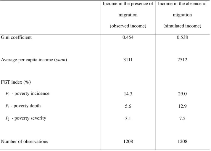
(24) land area reaches 57 mus, which is far higher than the average value 7.9 mus (see Table 1). Farm income, hence, increases with land area in our case. As we expect, households in suburban areas are richer as specialization in commercial farming, measured by the percentage of vegetable field of the village, significantly contributes to increasing farmers’ income.. (Table 3). 7.2 Remittances, inequality and poverty We use the results of Regression 4 to simulate the counterfactual of how household incomes, poverty and inequality would have been in the absence of migration for all the households. Table 4 shows the comparison between observed income and predicted income. In the absence of migration, household per capita income would have been 19.3% lower, while Gini would haven been 18.5% higher. In other words, participation in migration not only increases household income but also lowers inequality in rural areas. Using the basic needs poverty line developed by Ravallion and Chen (2004) for rural areas, which is equal to 850 yuans in 2002, we find that remittances lead to a decline in the incidence of household poverty ( P0 ) from 29.0% to 14.3%, in the depth of poverty ( P1 ) from 12.9% to 5.6%, and in the severity of poverty ( P2 ) from 7.5% to 3.1%. The strong impacts on depth of poverty suggests that migration reduces the income gap among the poor; and those on the severity of poverty, which assigns higher weights to the poorest of the poor, suggests that migration improves the well-being of the poorest disproportionately. In other words, the gains in poverty reduction due to migration go disproportionately to the poorest households (de Braud and Giles, 2008).. 21.

(25) (Table 4). Decisions made by rural households concerning their involvement in migration generally depend on two main factors: the incentives offered and the household’s capacity (FAO, 1998). Incentives and capacity for undertaking migration may diverge. On the one hand, poor farmers may have strong incentives to participate in migration while lacking the capacity to do so because of various constraints; on the other hand, if participation in migration is costly and initially risky, wealthy households are in a more favorable position to diversify their members into external labor market, but their diversification incentives may be weaker due to higher opportunity costs. The relationship between household wealth and participation in migration is driven by the two forces in different directions and may be not linear. Following Du et al. (2005), we estimate nonparametrically the relationship between observed migration participation and simulated household income in the absence of migration. As the simulated income does not include the contribution of migration, it can be considered as completely exogenous in this specification. Figure 1 shows the results of “potential migration propensity” by income level.. (Figure 1). The relationship between migration probability and simulated household income is nonlinear. The inverse-U shape association indicates that at low income levels, the likelihood of migration increases with income; then it decreases after peaking at about 65% at the income level of 6.5 in logarithmic form. The propensity of migration is relatively low for the rich households. This result tends to suggest that although the poor households may have higher incentive to participate in migration, a minimum level of productive resources is required to take advantage of new 22.

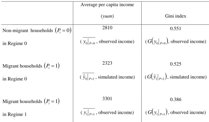
(26) migration opportunities. However, a higher propensity to participation in migration among poorer households does not necessary imply that they benefit more from migration. To examine the changes in income distribution resulted from migration across the population, we present the difference between observed income and predicted income for all households and migrants households, respectively, in a growth incidence curve (GIC) format in Figure 2. The curves show the changes in per capita income resulted from migration for each segment of population. As the GIC is above the zero axis at all points, income growth was positive for the entire population. All households benefit in the presence of migration. A strictly negative-sloped GIC, which displays changes in household per capita income of each percentile ranked from poor to rich, indicates that the poorer households experienced a higher rate of growth due to migration. For the poorest group (below the 25th percentile), household per capita income increased more than 80%; while that of the richest group (above 75th percentile), increased less than 25%. If we restrict the sample to migrant households, the amplitude of income growth is more important for the poorer ones.. (Figure 2). Table 5 shows income distribution of migrant households and non-migrant households under different scenarios. In the absence of migration (regime 0), per capita income of migrant households (2323 yuans) would have been lower than that of non-migrant households (2810 yuans), while levels of income inequality within migrant households and within non-migrant households are similar. Income premiums of the farmers who choose to stay in local production is 21% higher than those who choose to migrate. For the migrant households, their expected income from local production is lower; but participating in migration raises significantly their average 23.

(27) living standard. Hence, migration is a long-term rational choice of the rural households. The households that choose to concentrate on local production are usually those with comparative advantages in rural areas and with higher expected home earnings. However, in the presence of migration (regime 1), the level and distribution of income of migrant households both significantly improve. As the poorer households benefit disproportionately, migration contributes to lower income inequality among all households and within migrant households. One reason could be that poor households are more likely to suffer from the binding constraints, such as lower level of land resource per capita. They may face cornered solutions as their abilities to weather negative shocks are weaker. If those currently employed in the urban sector were engaged in some alternative employment, such as being agricultural labor, agricultural wage rates might be lower and overall income inequality might rise. Rather than raising inequality, migration actually contributes to prevent inequality from rising even further (Barrett et al., 2001; Chapman and Tripp, 2004).. (Table 5). Finally, we illustrate the income distribution of two kinds of households under different scenarios, using the estimators of Kernel density. Figure 3 shows that, in the absence of migration (in regime 0), the income distribution of households that participate in migration (population B) would be to the left of that of non-migrant households (population A): the average income of the former would be lower than that of the latter. When population B participates in migration (regime 1, becoming population C), the center of the distribution of their incomes largely moves to the right, beyond that of non-migrant households (population A), and inequality in their total income distribution declines. It is hence the households who would be poorer with only local 24.

(28) activities that benefit more from migration; and, in the presence of migration, their incomes are in average higher than those of non-migrant households. This equalizes income distribution.. (Figure 3). 8 Conclusions Migration has played an important role in increasing income level and changing income distribution in rural China since the economic reforms. Urban employment not only offers migrant workers alternatives job opportunities, but also helps alleviate the pressure of land shortage on those remain in countryside. As credit market and insurance market are highly inefficient in China, many poor rural households are not able to optimize their investments in physical and human capitals due to binding constraints of shortage in resources. In this circumstance, migration not only provide household with inflows of resource to invest in farming activities, but also serve as an insurance system to mitigate income fluctuations (Stark, 1980). A large amount of rural labor spontaneously chooses to migrate to urban areas to seek better opportunities. Our results first show that migration income, considered as a “potential substitute” for home income, tends to have an egalitarian effect on earnings in rural China. Migration provides the possibility for the households with low marginal labor productivity in rural areas to diversify their production in urban sector and hence increase income. Households with larger labor endowment relative to land resources, which would have been in general poorer in the absence of migration, are more likely to participate in migration as their opportunity costs are lower. Second, our results indicate that participation in migration noticeably reduced rural poverty. 25.

(29) Migration raises the income of poor households to a larger extent than that of rich households. Poverty headcount, poverty depth, and poverty severity are significantly lower in the presence of migration in this case study in Hubei province. In rural China, with no ownership but only usufruct of the land, a land market does not exist. Hence, farm income is relatively fixed because it is difficult to increase farm size. Therefore, migration serves as a solution for the absorption of rural surplus labor and remittances provide rural households with an additional source of income, improving their living standards and narrowing income gaps as well. Third, we find that shortage of land, education, and proximity to economic centers are important factors that encourage households to participate in migration. Non-migrant households are more productive in local production than migrant households due to observable and nonobservable characteristics, implying a rational selection. We argue that, the two observations that many existing studies rely on – (i) the distribution of non-farm income is more unequal than the distribution on farm-income in rural areas; and (ii) the average observed income of migrant households are higher than that of non-migrant households – do not provide adequate support to conclude that non-farm income increases inequality. First, as most rural household have farm income but not all rural households have non-farm income, it is normal that the distribution of non-farm income is more unequal. However, this does not necessarily suggest that, in relative terms, poor households have lower non-farm income. The relationship between urban-to-rural migration income and home earnings can be both substitute and complement. Our results show that this relationship makes the distribution of total income prone to be more equal than that of income in the absence of migration. Second, a higher observed average income of migrant households than that of non-migrant households does not necessarily suggest that households that choose to migrate would have had higher income in the absence to migration. Our analysis shows that, if these households did not participate in migration, 26.

(30) their income would have been lower than that of non-migrant households. The households that choose to stay in rural area are those with a comparative advantage in farming and with higher expected rural income. Migration in fact offers opportunities for households to make rational choice in optimizing income strategies given their observable and unobservable attributes, and the returns to these attributes given where they live. Implementation of the Household Responsibility System in the late 1970s undoubtedly raised agricultural productivities and set stage for the economic reforms. However, as household became a basic economic unit and household size became criteria for land allocation, land was divided into small plots for cultivation, which seriously impedes agricultural modernization as the economy develops. Given the natural endowments and technology conditions in China, agricultural development cannot mainly rely on land area increase or on technical improvement in the short run. Consolidating plots to exploit economy of scale may be a main source of gains in agricultural productivity. Agricultural labor productivity is likely to remain low. Migration serves as a rational self-selection – more productive farmers stay in countryside while worker with higher expected return in urban sectors migrate. Appropriate policy reforms that allow the market to play a better role in allocating land to productive farmers, and alleviate the barriers of migration to increase labor productivity would be important for improving living standards and reducing income inequality in rural China.. References Adams, R. H. Jr., 1989. Worker Remittances and Inequality in Rural Egypt. Economic Development and Cultural Change, 38(1), 45-71.. 27.

(31) Adams, R. H. Jr., 1994. Non-Farm Income and Inequality in Rural Pakistan: A Decomposition Analysis. The Journal of Development Studies, 31(1), 110-133. Adams, R. H. Jr., 1998. Remittances, Investment, and Rural Asset Accumulation in Pakistan. Economic Development and Cultural Change, 47, 155-173. Adams, R. H. Jr., 1999. Non-farm Income, Inequality and Land in Rural Egypt. Policy Research Working Paper 2178, The World Bank, Washington D. C. Adams, R. H. Jr., He, J. J., 1995. Sources of Income Inequality and Poverty in Rural Pakistan. IFPRI Research Report 102, Washington, D. C. Adams, R. H. Jr., Page, J., 2003. International Migration, Remittances and Poverty in Developing Countries. Policy Research Working Paper No. 3179, The World Bank (Poverty Reduction Group), Washington, D. C. Ahlburg, D. A., 1996. Remittances and the Income Distribution in Tonga. Population Research and Policy Review, 15(4), 391-400. Aubert, C., 1995. Exode rural, exode agricole en Chine, la grande mutation?. Espace Populations Société, 1995-2, 231-245. Banister, J., Taylor, J. R., 1990. China: Surplus Labour and Migration. Asia-Pacific Population Journal, 4(4), 3-20. Barham, B., Boucher, S., 1998. Migration, remittances, and inequality: estimating the effects of migration on income distribution. Journal of Development Economics, 55(2), 307-331. Barrett, C. B., Reardon, T., Webb, P., 2001. Nonfarm Income Diversification and Household Livelihood Strategies in Rural Africa: Concepts, Dynamics, and Policy Implications. Food Policy, 26(4), 315-331. Bhalla, A. S., 1990. Rural-Urban Disparities in India and China. World Development, 18(8), 1097-1110. 28.

(32) Bright, H., Davis, J., Janowski, M., Low, A., Pearce, D., 2000. Rural Non-Farm Livelihoods in Central and Eastern Europe and Central Asia and the Reform Process: A Literature Review. World Bank Natural Resources Institute Report No. 2633, The World Bank, Washington D. C. Carr, E. H., Davies, R. W., 1971. A History of Soviet Russia: Foundations of a Planned Economy, 1926-1929. Macmillan, London. Chapman, R., Tripp, R., 2004. Background Paper on Rural Livelihood Diversity and Agriculture. mimeo, AgREN electronic conference on the Implications of Rural Livelihood Diversity for Pro-poor Agricultural Initiatives. Chen, S., Wang, Y., 2001. China’s growth and poverty reduction: recent trends between 1990 and 1999. Paper presented at a WBI-PIDS Seminar on “Strengthening Poverty Data Collection and Analysis” held in Manila, Philippines, April 30-May 4, 2001. Chinn, D. L., 1979. Rural Poverty and the Structure of Farm Household Income in Developing Countries: Evidence from Taiwan. Economic Development and Cultural Change, 27(2), 283301. Chotikapanich, D., Rao, D. S. P., Tang, K. K., 2007. Estimating income inequality in China using grouped data and the generalized beta distribution. Review of Income and Wealth, 53(1), 127147. Davin, D., 1999, Internal Migration in Contemporary China. St. Martin’s Press, Inc., New York. de Beer, P., Rocca, J-L., 1997. La Chine à la fin de l’ère DENG Xiaoping. Le Monde-Editions, Paris. de Braud, A., Giles, J., 2008. Migrant Labor Markets and the Welfare of Rural Households in the Developing World: Evidence from China. Seminar at the Social Protection and Labor Sector of the Human Development Network of the World Bank, Washington, D. C. de Janvry, A., Sadoulet, E., 2001. Income Strategies Among Rural Households in Mexico: The 29.

(33) Role of Off-farm Activities. World Development, 29(3), 467-480. de Janvry, A., Sadoulet, E., Zhu, N., 2005. The Role of Non-Farm Incomes in Reducing Rural Poverty and Inequality in China. CUDARE Working Papers 1001, University of California, Berkeley, available at http://repositories. cdlib. org/are_ucb/1001. Du, Y., Park, A., Wang, S., 2005. Migration and rural poverty in China. Journal of Comparative Economics, 33(4), 688-709. Elbers, C., Lanjouw, P., 2001. Intersectoral Transfer, Growth, and Inequality in Rural Ecuador. World Development, 29(3), 481-496. Escobal, J., 2001. The Determinants of Nonfarm Income Diversification in Rural Peru. World Development, 29(3), 497-508. FAO, 1998. The state of food and agriculture 1998. FAO, Rome. Foster, J., Greer, J., Thorbecke, E., 1984. A Class of Decomposable Poverty Measures. Econometrica, 52(3), 761-766. Heckman, J., 1979. Sample selection bias as a specification error. Econometrica, 47(1), 153-161. Hussain, A., Lanjouw, P., Stern, N., 1994. Income Inequalities in China: Evidence from Household Survey Data. World Development, 22(12), 1947-1957. Islam, N., 1997. The non-farm sector and rural development – review of issues and evidence. Food, Agriculture and the Environment Discussion Paper 22. IFPRI, Washington D. C. Jones, R. C., 1998. Remittances and inequality: A question of migration stage and geographic scale. Economic Geography, 74 (1), 8-25. Kanbur, R., Zhang, X., 1999. Which regional inequality? The evolution of rural-urban and inland-coastal inequality in China, 1983-1995. Journal of Comparative Economic, 27(4), 686701. 30.

(34) Khan, A. R., Riskin, C., 2001. Inequality and poverty in China in the age of globalization. Oxford University Press, New York. Kimhi, A., 1994. Quasi Maximum Likelihood Estimation of Multivariate Probit Models: Farm Couples’ Labor Participation. American Journal of Agricultural Economics, 76(4), 828-835. Knight, J., Song, L., 1993. The spatial contribution to income inequality in rural China. Cambridge Journal of Economics, 17(2), 195-213. Lachaud, J-P., 1999. Envois de fonds, inégalité et pauvreté au Burkina Faso. Revue Tiers Monde, 40(160), 793-827. Lanjouw, P., 1999a. The Rural Non-Farm Sector: A Note on Policy Options. Non-Farm Workshop Background paper, The World Bank, Washington D. C. Lanjouw, P., 1999b. Rural Non-Agricultural Employment and Poverty in Ecuador. Economic Development and Cultural Change, 48(1), 91-122. Leones, J. P., Feldman, S., 1998. Nonfarm Activity and Rural Household Income: Evidence from Philippine Microdata. Economic Development and Cultural Change, 46(4), 789-806. Liu, H., 2006. Changing reginal rural inequality in China 1980-2002. Area, 38(4), 377-389. Lopéz, R., Schiff, M. 1995. Migration and Skill Composition of the Labor Force : The Impact of Trade Liberalisation in Developing Countries. The World Bank Working Paper 1493, The World Bank, Washington D. C. McKenzie, D. J., 2005. Beyond Remittances: The effects of Migration on Mexican Households. in C. Ozden, M. Schiff, eds, International Migration, Remittances and the Brain Drain. The World Bank, Washington D. C. Mckenzie, D., H. Rapoport, 2007. Network effects and the dynamics of migration and inequality: Theory and evidence from Mexico. Journal of development Economics, 84 (1), 1-24. McMillan, J., Whalley, J., Zhu, L., 1989. The Impact of China’s Economic Reforms on 31.

(35) Agricultural Productivity Growth. Journal of Political Economy, 97(4), 781-807. Naughton, B., 1999. Causes et conséquences des écarts de croissance entre provinces. Revue d’économie du développement, 1999-1/2, 33-70. National Bureau of Statistics of China, 2005. China Statistical Yearbook 2005. China Statistics Press, Beijing. OECD, 2005. Migration, Remittances and Development. OECD Publishing, Paris. Pyatt, G., Chen, C., Fei, J., 1980. The Distribution of Income by Factor Component. Quarterly Journal of Economics, 95(3), 451-473. Ravallion, M., 2005. Externalities in Rural Development: Evidence for China. in R. Kanbur, T. Venables, eds, Spatial Inequality. Oxford University Press. Ravallion, M., Chen, S., 2001. Measuring Pro-Poor Growth. Policy Research Working Paper, No. 2666, The World Bank, Washington D. C. Ravallion, M., Chen, S., 2004. China’s (Uneven) Progress Against Poverty. Working Paper Series No. 3408, The World Bank, Washington D. C. Reardon, T., Taylor, J. E., 1996. Agro-climatic Shock, Income Inequality, and Poverty: Evidence from Burkina Faso. World Development, 24(5), 901-914. Rodriguez, E., 1998. International Migration and Income Distribution in the Philippines. Economic Development and Cultural Change, 46(2), pp. 329-350. Rural Economic Research Center, The Ministry of Agriculture of China, 2003, Chinese Rural Research Report 2001. China Financial & Economic Publishing, Beijing. Schiff, M., 1996. South-North Migration and Trade. The World Bank Working Paper No. 1696, The World Bank, Washington D. C. Schultz, T. W., 1964. Transforming Traditional Agriculture. Yale University Press, New Haven.. 32.

(36) Shand, R. T., 1987. Income Distribution in a Dynamic Rural Sector: Some Evidence from Malaysia. Economic Development and Cultural Change, 36(1), 35-50. Stark, O., 1980. Urban-to-Rural Remittances in Rural Development. Journal of Development Studies, 16(3), 369-374. Stark, O., 1991. The Migration of Labor. Basil Blackwell, Oxford. Stark, O., Taylor, J. E., Yitzhaki, S., 1986. Remittances and Inequality. Economic Journal, 96(383), 722-740. Stark, O., Taylor, J. E., Yitzhaki, S. 1988. Migration Remittances and Inequality: A Sensitivity Analysis using the Extended Gini Index. Journal of Development Economics, 28(3), 309-322. Straubhaar, T., Vadean, F. P., 2005. Introduction: International Migrant Remittances and their Role in Development. in OECD, Migration, Remittances and Development. OECD Publishing, Paris. Taylor, J. E., 1992. Remittances and inequality reconsidered – direct, indirect and intertemporal effects. Journal of Policy modeling, 14 (2), 187-208. Taylor, J. E., 1999. The New Economics of Labor Migration and the Role of Remittances. International Migration, 37(1), 63-88. Taylor, J. E., Yunez-Naude, A., 1999, Education, migration et productivité: une analyse des zones rurales au Mexique. Centre de Développement de l’OCDE, Paris. Taylor, J. E., Wyatt, T. J., 1996. The Shadow Value of Migrant Remittances, Income and Inequality in a Household-farm Economy. Journal of Development Studies, 32(6), 899-912. The World Bank, 2000. Can Africa Claim the Twenty-First Century. The World Bank, Washington D. C. The World Bank, 2005. China: Integration of national product and factor markets – economic benefits and policy recommendations. The World Bank, Washington D. C. 33.

(37) The World Bank, 2007. World Development Report 2008: Agriculture for Development. The World Bank, Washington D. C. Wade, R. H., 2004. Is Globalization Reducing Poverty and Inequality?. World Development, 32(4), 567-589. Wan, G., 2004. Accounting for income inequality in rural China: a regression-based approach. Journal of Comparative Economics, 32(2004), 348-363. Wan, G., Zhou, Z., 2005. Income Inequality in Rural China: Regression-based Decomposition Using Household Data. Review of Development Economics, 9(1), 107-120. Yao, S., 1999. Economic Growth, Income Inequality and Poverty in China under Economic Reforms. Journal of Development Studies, 35(6), 103-130. Zhang, Y., Wan, G., 2006. The impact of growth and inequality or rural poverty in China. Journal of Comparative Economics, 34(2006), 694-712. Zhao, Y., 1999. Leaving the Countryside: Rural-to-Urban Migration Decision in China. The American Economic Review, 89(2), 281-286. Zhu, L., 1991. Rural Reform and Peasant Income in China. Macmillan, London. Zhu, L., Jiang, Z., 1993. From brigade to village community: the land tenure system and rural development in China. Cambridge Journal of Economics, 17(4), 441-461. Zhu, N., 2002a. Analyse des migrations en Chine: mobilité spatiale et mobilité professionnelle, Thèse pour le Doctorat en Sciences Economiques, présentée et soutenue publiquement le 26 novembre 2002, CERDI, Clermont-Ferrand, France. Zhu, N., 2002b. Pauvreté, inégalité et croissance du secteur non-agricole rural en Chine. in J-M. Dupuis, C. El Moudden, F. Gavrel, I. Lebon, G. Maurau, N. Ogier, Politiques sociales et croissance économique. L’Harmattan, Paris/Budapest/Torino. Zhu, N., Luo, X., 2006. Non-farm activity and rural income inequality: a case study of two 34.

(38) provinces in China. Policy Research Working Paper No. 3811, The World Bank, Washington D. C.. 35.

(39) Tables and figures. Table 1 - Descriptive statistics All. Non-migrant. Migrant. households. households. households. Difference. 12867. 10506. 14360. -3854 *** (-5.18). Home income (yuan). 8017. 10506. 6443. 4063 *** (6.39). Remittances (yuan). 4850. Total income (yuan). 7917. 3111. 2810. 3301. -492 ** (-2.32). 2.8. 2.4. 3.1. -0.6 *** (-8.59). Number of farm workers. 1.7. 2.0. 1.5. 0.5 *** (7.44). Number of local non-farm workers. 0.3. 0.4. 0.2. 0.2 *** (5.49). Number of migrants. 0.8. Per capita income (yuan). Number of workers. 1.4. Average number of years of education. 7.0. 6.6. 7.3. -0.7 *** (-4.92). Number of dependents. 1.3. 1.4. 1.2. 0.2 *** (2.82). Number of children. 0.1. 0.1. 0.2. -0.1 *** (-3.02). Land area (mu). 7.1. 7.9. 6.6. 1.2 *** (2.58). Per capita land area (mu). 2.8. 3.5. 2.4. 1.1 *** (5.28). 5.4. 7.0. 4.3. 2.7 *** (5.77). 20.6. 23.4. 18.9. 4.5 *** (4.22). 7.2. 8.3. 6.5. 1.8 *** (4.39). Per capita gross output value of the village (yuan). 3370. 3329. 3396. -67. Percentage of non-farm production of the village (%). 27.7. 25.6. 29.0. -3.4 *** (-2.78). Cultivable land per capita of the village (mu). 1.2. 1.2. 1.2. Percentage of paddy field of the village (%). 21.1. 19.4. 22.2. Percentage of vegetable field of the village (%). 19.2. 19.3. 19.2. Number of observations. 1208. 468. 740. Distance from household’s residence to the nearest bus station (km) Distance from household’s residence to the county capital (km) Distance from household’s residence to the nearest rural market (km). 0.0. (-0.60). (0.41). -2.8 *** (-3.04) 0.1. (0.10). Note: (1) t-statistics are in brackets. *** significant at 1%; ** significant at 5%; * significant at 10%. (2) One yuan = 0.12 US$; one mu is equal to 1/15 hectares.. 36.

(40) Table 2 - Estimation of the participation equation (Probit). Endogenous variable = 1 if household participates in migration Regression 1 For all households Number of workers in the household. 0.273 ***. (8.06). 6-9 years. 0.261 ***. (2.68). 9-12 years. 0.509 ***. (4.80). Average number of years of education (ref.: 0-6 years). 12 years or above. -0.410. (-1.46). Number of dependents. -0.052. (-1.49). 0.147. (1.34). Number of children under five Land area of the household. -0.015 ***. (-2.89). Distance from household’s residence to the nearest bus station. -0.020 ***. (-3.59). Distance from household’s residence to the county capital. -0.007 **. (-2.41). Distance from household’s residence to the rural fair. -0.003. (-0.36). Logarithm of per capita gross output value of the village. -0.051. (-0.63). Proportion of non-farm production of the village (/100). 0.021. (0.09). -0.017. (-0.27). 0.229. (0.69). Proportion of vegetable field of the village (/100). -0.156. (-0.55). Constant. -0.350. (-1.30). Cultivable land per capita of the village Proportion of paddy field of the village (/100). Maximum likelihood in log. -725.218. Pseudo- R 2. 0.101. Percentage of correction predictions (%). 67.4. Number of observations. 1208. Note: t-statistics are in brackets. *** significant at 1%; ** significant at 5%; * significant at 10%.. 37.

(41) Table 3 - Estimation of the income equation (OLS) Endogenous variable: logarithm of household per capita income. Number of household’s workers Average number of years of education (ref.: 0-6 years) 6-9 years 9-12 years 12 years or above Number of dependents Number of children Land area of the household Squared land area of the household (/100) Logarithm of per capita gross output value of the village Proportion of non-farm production of the village (/100) Cultivable land per capita of the village Proportion of paddy field of the village (/100) Proportion of vegetable field of the village (/100) Distance from household’s residence to the nearest bus station Distance from household’s residence to the county capital Distance from household’s residence to the rural fair Inverse Mills Ratio Constant. Only for non-migrant households In the absence of Inverse Mills Ratio In the presence of Inverse Mills Ratio Regression 2 Regression 3 Regression 4 0.031 (0.76) 0.296 (1.24) 0.014 (0.21). 0.460 0.485 0.887 -0.093 -0.406 0.040 -0.035. *** (4.11) 0.693 *** (2.94) *** (3.78) 0.966 ** (2.17) *** (3.26) 0.550 (1.36) ** (-2.29) -0.139 ** (-2.41) *** (-2.72) -0.255 (-1.27) *** (3.76) 0.025 (1.55) ** (-2.24) -0.033 ** (-2.14). 0.180 **. 0.135. (1.39). (-1.25) -0.322 (1.01) 0.049. (-1.16) (0.64). 0.038. (0.09). 0.270. (0.59). 1.272 ***. (3.69). 1.133 ***. (3.10). -0.345 0.075. -0.005 …. (2.04). (-0.93) -0.023. (-1.37). (0.02). (-0.96). -0.007. (-0.53) -0.007 (-0.83) 1.469 (1.12) 6.903 *** (22.70) 7.765 *** (9.42). 0.457 0.465 0.892 -0.091 -0.396 0.041 -0.036. *** *** *** ** *** *** **. (3.81) (2.89) (3.21) (-2.17) (-2.63) (3.81) (-2.36). 0.188 ** (2.27). -0.003. (-0.01). 1.303 *** (4.26). -0.004. -0.091 (-0.30) 6.799 *** (28.07). 0.209 0.211 0.202 R2 Number of observations 468 468 468 Note: t-statistics in brackets. *** significant at 1%; ** significant at 5%; * significant at 10%. “…” means that the absolute value is inferior to 0.001.. 38.

(42) Table 4 - Comparison of income distribution with and without migration. Income in the presence of Income in the absence of migration. migration. (observed income). (simulated income). Gini coefficient. 0.454. 0.538. Average per capita income (yuan). 3111. 2512. P0 - poverty incidence. 14.3. 29.0. P1 - poverty depth. 5.6. 12.9. P2 - poverty severity. 3.1. 7.5. 1208. 1208. FGT index (%). Number of observations Note: Poverty line is equal to 850 yuans.. 39.

(43) 0. .2. .4. .6. .8. 1. Figure 1 - Migration participation and household income. 4. 6 8 10 Simulated income in the absence of migration (logarithmic scale). 12. bandwidth = .5. 40.

(44) 150 100 0. 50. Income increase (%). 200. Figure 2 - Growth incidence curve: effect of migration on changes in household income. 0. 25 50 75 Percentile of the households (ranked by per capita household income) GIC for all households. 100. GIC for migrant households. 41.

(45) Table 5 – Income distribution of migrant households and non-migrant households in different regimes. Average per capita income. Non-migrant households Pi  0 in Regime 0. ( y0. P 0. Migrant households Pi  1 in Regime 0. Gini index. 2810. 0.551. , observed income). . ( G y0. P 0. 2323 ( yˆ 0. P 1. Migrant households Pi  1 in Regime 1. (yuan). , simulated income). 0.525. . ( G yˆ1. P 1.  , simulated income). 3301 ( y1. P 1. , observed income). , observed income). 0.386. . ( G y1. P 1.  , observed income). 42.