Trade Liberalization, Inequality and Poverty in Brazilian States

HAL Id: halshs-00967356

https://halshs.archives-ouvertes.fr/halshs-00967356

HAL is a multi-disciplinary open access

archive for the deposit and dissemination of sci-entific research documents, whether they are pub-lished or not. The documents may come from teaching and research institutions in France or abroad, or from public or private research centers.

L’archive ouverte pluridisciplinaire HAL, est destinée au dépôt et à la diffusion de documents scientifiques de niveau recherche, publiés ou non, émanant des établissements d’enseignement et de recherche français ou étrangers, des laboratoires publics ou privés.

Trade Liberalization, Inequality and Poverty in Brazilian

States

Marta Castilho, Marta Menéndez, Aude Sztulman

To cite this version:

Marta Castilho, Marta Menéndez, Aude Sztulman. Trade Liberalization, Inequality and Poverty in Brazilian States. 2010. �halshs-00967356�

Trade Liberalization,

Inequality and Poverty

in Brazilian States

Marta CASTILHO

Univ. Federal Fluminense Université Paris-Dauphine Marta MENENDEZ IRD DIAL

Paris School of Economics

Aude SZTULMAN Université Paris-Dauphine

IRD DIAL

G-MonD

Working Paper n°6

Trade Liberalization, Inequality and Poverty in Brazilian States

Marta Castilho

, Marta Menéndez

* and Aude Sztulman

a

Universidade Federal Fluminense, Brazil

b

Université Paris-Dauphine, LEDa-DIAL, 75775 Paris cedex 16, France

c

IRD, UMR 225 DIAL, 75010, France

d

Paris School of Economics, France

Abstract

This paper studies the impact of globalization on household income inequality and poverty using detailed microdata across Brazilian states from 1987 to 2005. Results suggest that the Brazilian states more exposed to tariff cuts experienced smaller reductions in household poverty and inequality. Contrasting results emerge when we disaggregate into rural and urban areas within states: trade liberalization contributes to growth in poverty and inequality in urban areas and may be linked to reductions in inequality in rural areas. In terms of observed integration into world markets, we find evidence indicating that state poverty and inequality in Brazil decrease with rising export exposure and increase with import penetration.

Keywords: Trade liberalization, poverty and inequality; Latin America; Brazilian states. JEL codes: D31, F16, F14

1. Introduction

How globalization affects income distribution remains a keenly discussed topic in today’s academic and policy circles. Back in the 1980s, the policy debate essentially concerned industrialized countries seized by rising inequalities and increased international competition on domestic markets. Since then, trade reforms in a number of developing and emerging countries and the growing availability of datasets have led to more studies on the distributional and social effects of international trade on countries from the developing world. The debate is partially motivated by the complexity of

†

The authors are particularly indebted to Nina Pavcnik for careful reading and thoughtful comments. This paper has benefited from helpful discussions with Barbara Coello, Jean-Marc Siroën and participants at conferences and seminars. The authors are grateful to Honorio Kume for kindly providing us with tariffs data and to Pierre-Emmanuel Couralet and Jeremie Gignoux for their help in building harmonized data series from PNAD surveys.

*

Corresponding author: Marta Menéndez, Université Paris-Dauphine, Place du Maréchal de Lattre de Tassigny, bureau P301bis, 75 775 Paris cedex 16, France. E-mail: marta.menendez@dauphine.fr; Tel: +33 1 44054460; Fax: +33 1 44054733.

the channels through which globalization – an all-encompassing term used here to include trade liberalization and integration into world markets – affects inequality and poverty within a country (see Goldberg and Pavcnik, 2004, 2007; Winters et al., 2004; and Ferreira et al., 2007a, for an overview of the various trade transmission mechanisms).

In this paper, we study the impact of trade liberalization and international trade on household income inequality and poverty using detailed microdata across Brazilian states from 1987 to 2005. We seek to gauge whether Brazilian states with greater exposure to trade over these two decades exhibited differential changes in their income distribution, both in terms of poverty and inequality levels.

This paper makes several contributions to the literature on globalization and income distribution. Firstly, it is one of the few studies to consider both trade policy variables and international trade flow variables to assess the distributional impacts of trade within a country. The implementation of these two approaches allows us to thoroughly seize the effects of globalization on poverty and inequality.

Secondly, using subnational units of observation (Brazilian states in our case, together with a distinction between in-state rural and urban areas), this study analyzes the Brazilian economy taking into account regional differences. By adopting this regional approach, our paper adds to the recent strand of research that includes a spatial dimension in its study of the impact of trade liberalization on income distribution in a country (see Wei and Wu (2002) on China; Topalova (2005) on India; McCaig (2009) on Vietnam; Nicita (2004) on Mexico).1

Thirdly, the distributional measures considered in this paper are broader than those generally examined in previous studies. Although trade reforms should ultimately affect household welfare, it is only recently that some studies have considered measurements over and above wage inequality and the skill premium (Topalova, 2005; Porto, 2003 & 2006; Ferreira et al., 2007a; McCaig, 2009). Past publications’ focus on the skill premium is not surprising. It stems essentially from the predictions of the classical Heckscher-Ohlin-Samuelson (HOS) model. The HOS model posits that trade liberalization in poor countries should raise relative demand for unskilled labor (usually relatively abundant in these countries) and in turn reduce wage inequality and eventually reduce poverty. The HOS model’s predictions have nevertheless been challenged by empirical studies on some Latin American countries, where a combination of a rising skill premium and deteriorating income

distribution seemed to occur during periods of trade liberalization (see, for example, Robbins (1996) and Goldberg and Pavcnik (2007) for studies on various Latin American countries; Goldberg and Pavcnik (2005) and Attanasio et al. (2004) for Colombia; and Hanson (2003) for Mexico). Recent research concludes that we need to go beyond the scope of the HOS model predictions to evaluate the impact of globalization on income distribution within a country.2

Solely focusing on wages and the skill premium has additional shortcomings when considering developing countries with relatively high levels of poverty and very unequal distributions according to international standards, as is often the case in Latin America (WDR, 2006). Among other things, developing countries have a larger non-wage working population and a large informal sector. Broader welfare measurements to study the impact of trade liberalization have rarely been used, however, due to design and measurement problems and because comparable household poverty and inequality trends in developing countries are not always feasible or easy to produce (Goldberg and Pavcnik, 2004 & 2007).3

The few empirical studies that have attempted to link trade liberalization with household income inequality or poverty find contrasting results, depending on the methodology and country studied. For example, Topalova (2005) uses a regional approach and finds that trade liberalization from 1987 to 1997 raised poverty yet had no effect on inequality in rural Indian districts. She also finds that trade exposure had no impact on district inequality and poverty in urban India. McCaig (2009) obtains similar results from a study of short-run effects on Vietnamese provinces: between 2002 and 2004, provinces more exposed to tariff cuts appear to have experienced lower reductions in poverty, while increased access to US export markets caused greater drops in poverty. However, Porto (2003 & 2006) uses a different methodological approach and finds that trade reforms in Argentina had a positive impact on the poor.4 Porto (2003) shows that trade reforms and better access to foreign markets have a poverty-decreasing effect. Porto (2006) finds evidence of a pro-poor bias of the Mercosur trade agreement on Argentine families in the 1990s. The fact that different conclusions are reached in different countries encourages us to examine the matter with regard to Brazil, a case study that is of particular interest.

Brazil is remarkably well suited to an analysis of the impact of globalization on income distribution and poverty for a number of reasons. Firstly, Brazil embarked on an extensive trade liberalization reform in 1988, including a substantial widespread reduction in trade barriers and a narrowing of tariff dispersion. In the late 1980s, imports were subject to both very high tariff barriers and significant non-tariff barriers. Trade reforms started in 1988, and the average (unweighted) non-tariff fell from 40.4% in 1988 to 11.1% in 2005. These major changes in trade protection and other macroeconomic factors led to an increase in trade openness for Brazil and its different states (see section 2 below for a more detailed description of the changes in trade policies and trade patterns).

Secondly, Brazil, where poverty is very high and well above the norm for a middle income country, is one of the most inegalitarian countries in the world. During the period of interest, both welfare indicators started to decline slowly but significantly. Still, there are large inequality and poverty differences across rural and urban areas and across Brazilian states, in terms of both levels and trends (see section 3 below for a more detailed description of the progression of poverty and inequality indicators).

Thirdly, among the Latin American countries, Brazil seems to be a special case, at least as far as the studies examining the effects of trade liberalization on wage and employment outcomes are concerned. In Brazil, the economy-wide skill premium fell between 1988 and 2004 (Ferreira et al., 2000a) and recent studies find either no evidence of or a downward effect of trade liberalization on wage inequality.5 One reason that could account for these results is the nature of the Brazilian structure of protection prior to liberalization and how it has changed. Contrary to some other Latin American countries – for example Mexico (Hanson, 2003) and Colombia (Attanasio et al., 2004) – pre-liberalization tariffs in Brazil were higher in industries relatively intensive in skilled labor (Gonzaga et

al., 2006; Ferreira et al., 2007a). The objective of the Brazilian government was to reduce tariffs

across industries to more uniform rates. Consequently, tariff reductions were greater in skill-intensive industries (Gonzaga et al., 2006). In keeping with the Stolper-Samuelson predictions, this could explain how trade liberalization contributed to a reduction in inequality.

Finally, Brazil is politically organized as a federation composed of 27 federal units, namely 26 states plus the Distrito Federal or Federal District. As a large federal country, a relatively large

amount of intranational data is available. As regards the impact of trade openness, it is possible to measure, at state level, exposure both to tariff cuts (by weighting tariffs with the initial share of employment by industry within each state) and to international trade (data on exports and imports are available for each state). Hence, Brazil is among the few countries where we are able to study the effects of both tariff reductions and world market integration on state poverty and inequality, allowing an exhaustive assessment of the distributional impacts of trade within a country. Moreover, we will measure these trade policy and international trade flow variables at the sector level within states.

A technical, albeit no less important reason to study the Brazilian case is the fact that it benefits from the availability of very high-quality household datasets representative of almost the entire country and covering a period starting before trade liberalization. Long, reliable and comparable annual series can hence be established at household level and consequently at state level. As often pointed out, in-country studies do not suffer from the long list of data quality problems encountered by cross-country studies (such as differences in data definitions and collection methods leading to comparability problems across countries and time).

This paper shows that Brazilian trade liberalization raised poverty and inequality at state level, despite the fact that Brazilian states generally posted improvements in these welfare indicators over the period studied. In other words, Brazilian states that were more exposed to tariff cuts (i.e. had a greater share of workers in industries with large tariff cuts) experienced smaller reductions in household poverty and inequality. Although the significance of the results for the states as a whole seems contingent on the poverty and inequality indicators used, this is no longer the case when rural and urban areas are disaggregated within states. The effect of a tariff reduction is poverty and inequality increasing in urban areas but inequality reducing in rural areas (there is no significant effect on rural poverty). In terms of observed integration into world markets, the results are the opposite with regard to export exposure and import penetration. While import penetration plays a similar role to trade liberalization across Brazilian states as a whole, growing export exposure appears to reduce both poverty and inequality quite significantly.

The remainder of the paper is organized as follows. Section 2 provides a brief description of Brazilian trade reforms over the past two decades. Section 3 describes the dataset compiled for this

study (3.a) and presents descriptive statistics on trade patterns, poverty and inequality for Brazil as a whole and by federal unit. Section 4 describes the econometric specifications and estimation strategy (4.a) and includes an analysis of our findings on the impact of trade liberalization and international trade on poverty and inequality (4.b). Section 5 presents the conclusion of the study.

2. Trade reforms in Brazil

Brazilian trade policies have changed considerably over the past two decades. Through to the late 1980s, Brazil had a very restrictive trade regime led by a development strategy based on import substitution and the promotion of national industry. Not only was the level of protection high, but import policies were also particularly complex due to the use of countless trade instruments. This intricate system was reinforced by the fact that, in some circumstances, trade instruments were used for macroeconomic purposes without any connection with the original industrial and productive rationale. At the end of the 1980s – known as the “lost decade” by Latin American countries because of macro-instability and poor economic performance – the region started to adopt liberal public policies inspired by the Washington Consensus.6 The types and depth of the economic policies varied from country to country. In Brazil, the recommended policies were neither entirely nor simultaneously implemented, but in general trade and financial liberalization measures were adopted from the early 1990s onwards.

Trade reform in Brazil effectively started in 1988, when some non-tariff barriers were removed. At that time, the nominal tariff, measured by a simple cross-sector average (see Figure 1) stood at 40.4%, with a highly dispersed distribution (standard deviation of tariffs above 15%) and substantial “tariff redundancy”.7 With the arrival of the new government in 1990 came a hefty package of trade measures. The main goal of the reform was to rationalize the trade regime and make tariffs the main trade instrument. The reform duly eliminated non-tariff barriers still in place (such as prohibitions and quantitative controls), abolished the majority of special import regimes and then reduced the level and spread of import tariffs. A tariff reduction schedule was established with the goal of nominal tariffs standing at an average 18% and ranging from 0% to 40% by 1994. These Brazilian trade reforms were

initiated unilaterally in accordance with the country’s commitments in the ongoing multilateral negotiations (Uruguay Round). However, in 1991, Brazil signed the Mercosur agreement with Argentina, Paraguay and Uruguay. The four countries negotiated the Common External Tariff (CET), which called for certain amendments to be made to the original liberalization schedule. Under the Mercosur agreement, the average tariff fell to 12% in 1996 (with the standard deviation of tariffs falling to 7%) in a demonstration of the reach of the liberalization process.8

<Figure 1>

All in all, the 1990s Brazilian trade reforms not only achieved their goal of streamlining the import tariff structure, but also led to extensive tariff cuts and more uniform tariff rates. After the implementation of the CET in 1994, only small changes were made, mainly for the purposes of macroeconomic adjustment. The sharp growth in imports that followed the Real Plan (adopted in 1994) and the subsequent price stabilization called for certain quantitative and administrative measures to be enforced in 1996 to control the growing trade deficit.9 As of 1997, the Asian financial crisis had a strong impact on external accounts and made the Brazilian exchange rate unsustainable. In 1997, the country, together with its Mercosur partners, temporarily raised the CET by 3%10 and, in January 1999, the Brazilian currency’s face value was devalued by about 50%. While the expected impacts on exports and imports were not immediate, the measures put in place managed to halt the trade deficit’s upward spiral. From 2001 to 2004, the trade surplus grew from US$ 2 billion to US$ 33 billion.11 By 2005, the Brazilian tariff had reached its lowest ever level with a simple average tariff of 11.1%.

If we take a look at the tariff protection structure by sector for the 1987-2005 period, we can see the extent of the tariff cuts and reduction in spread (see Figure 2). The largest tariff cuts concerned the sectors where initial tariff levels were highest, i.e. manufacturing sectors such as automobiles, apparel and textiles. The smallest tariff cuts were made in the mining sectors, where initial tariff levels were lowest. Protection levels in the agricultural and food sectors – where Brazil has strong comparative advantage – were close to the Brazilian average tariff.12

<Figure 2>

Note that detailed information on non-tariff barriers (NTBs) is not available on a disaggregated basis to construct time series across sectors in Brazil and has not been included in this study. This

should not cause too much of a problem, considering that tariffs are the main policy instrument in Brazil. Although NTBs may have played a role as a trade barrier through to 1990, they have since become a relatively insignificant protectionist instrument.13

These changes in trade protection together with those in the macroeconomic environment and policies affected trade performance in Brazil as a whole and in the different Brazilian states. Figure 3 shows the three usual indicators of international trade exposure – trade openness, import penetration and export-to-output ratios – for Brazil. Since 1989, trade openness has more than doubled, reaching 26.4% in 2004 (compared to 11.8% in 1989 and 13.8% in 1998).14 Changes were more significant from 1999 onwards. The large increase in trade openness between 1998 and 2004 is mainly due to growth in exports, during which time export exposure rose by nearly 10% compared to around 4% for import penetration.

<Figure 3>

Given that our empirical framework studies the impact of trade openness at state level, a detailed description of trade exposure across Brazilian federal units is given in the next section following the presentation of our different datasets.

3. Trade, poverty and inequality in Brazil: data and descriptive analysis

3.a Data description

The data used in this study were provided by different sources. Household level microdata were gathered from our first source: the Pesquisa Nacional por Amostra de Domicílios (PNAD), which is conducted annually by the Brazilian Census Bureau (Instituto Brasileiro de Geografia e Estatística (IBGE)).15 The survey, which samples about 300,000 individuals every year, is nationally representative and covers the rural and urban areas of all states in the federation, except for the rural areas of the Northern Region where the Amazon rainforest is found.16 We use individual-level information from the PNAD to construct harmonized summary variables on income distribution, employment, education and other socio-demographic characteristics (detailed below) for our unit of

analysis, i.e. the state. Where appropriate, we make the distinction between rural and urban areas within states, for which all summary variables have been constructed as necessary.17

The definition of income used throughout the analysis is gross monthly household income per capita, measured in 2006 Brazilian reais, and the sample considered is the total population.18 Various measures of inequality and poverty have been considered for the sake of robustness. In the case of inequality, we have applied two common indicators: the Gini and Theil indices. When looking at poverty, two standard poverty indicators from the Foster-Greer-Thorbecke (FGT) metric have been calculated: the headcount index and the poverty gap.19 The first indicator captures the proportion of the population living below the poverty line and the second helps to account for differences among households in terms of their distance from the poverty line. For the purposes of this study, the poverty line is set at R$100 per person per month (2006 values). Robustness to the choice of threshold has been tested.20 In an effort to better gauge what is happening behind these summary statistics, we also calculate income levels across the income distribution quintiles (and deciles) and include them in our econometric study.

The PNAD provides individual data that can be used for our econometric analysis. We are able to observe, among other things, the labor market status of individuals in the population, as well as the sector in which they work.21 We are also able to consult a list of individual socio-demographic variables considered typical determinants of income levels. From these individual data, we can construct different control variables at state level (or rural/urban areas within states) and, in particular, the share of individuals in each state by years of schooling (grouped into six categories: none; 1 to 3 years; 4 to 7 years; 8 to 10 years; 11 to 14 years and 15 or more years); the share of individuals in each ethnic group (information on ethnicity is self-declared in the PNAD and defines five groups: indigenous, white, black, Asian and mixed); the share of the agricultural sector22 in each state; the share of informal workers; and the share of workers by industrial sector.

We use two different sets of measures to represent trade policy changes and the trade openness of Brazilian states. The first set includes trade policy measures, based on Brazilian nominal tariff data. The second set focuses on trade flows and shows the state’s exposure to international trade or its integration into world markets.

The trade policy data are made up of industry-specific nominal tariff rates. These are drawn from Kume et al. (2003) for the 1987-1994 period. Data were provided by H. Kume for 1995-2005. The tariff data series correspond to the nominal level of protection for 31 industry sectors.23 These data are a standard source for the Brazilian tariff structure.

Given that we adopt a regional approach, we follow Topalova (2005) and construct an indicator to measure the influence of trade policy and its change at state level in Brazil (and in urban and rural areas within states). This indicator, called LIB, is a weighted average of national industry-level tariffs, where the weights correspond to the initial share of employment by industry within each state (the initial year in our study is 1987). It is computed as follows:

1987 1987 ) ( s k kt sk st L Tariff L LIB

∑

where s denotes the unit of analysis (Brazilian states), k the sector and t time. Tariffkt refers to the tariff

in sector k for year t, Lsk1987 to the workers employed in sector k for year 1987 in unit of analysis s and Ls1987 to the total workers in unit of analysis s for the year 1987.

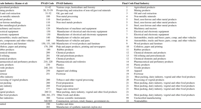
The weights are calculated using employment data on the year prior to the trade reform, i.e. 1987, to ensure that employment changes over time caused by tariff variations are not included in our LIB measure of exposure to the tariff reforms. The data on employment by federal unit and industry in 1987 were taken from the PNAD. Our use of household survey data and tariff data with different industry definitions called for concordance between the two datasets. To match the data on tariffs (in the Nivel 50 classification) and employment (in the PNAD classification), we used Table A1 of Industry Concordance (in the appendix) developed by Ferreira et al. (2007a). Consequently, we were able to compute our trade liberalization indicator LIB for a group of 22 industries in a sample of 26 states for the 1987-2005 period.24

The data on trade flows cover the following indicators: import penetration (imports as a percentage of output plus net imports); export exposure (exports as a percentage of output) and trade openness (defined as the ratio of imports plus exports to gross domestic product). These ratios are calculated at state level. No in-state urban-rural distinction can be made in this case. Trade data on the federal units’ imports and exports in current US dollars are collected by the Secretaria de Comércio Exterior,

Ministério do Desenvolvimento, Industria e Comércio Exterior (SECEX/MDIC).25

The series on gross domestic product by state in current market prices come from Brazil’s regional accounts as drawn up by IBGE. These data were converted into current US dollars using the annual average exchange rates.26 The trade flow indicators were calculated for total trade, but also separately for the agricultural sector and the industrial sector (the latter including the mining and manufacturing industries) for the 1989-2004 period.

3.b Trade, poverty and inequality in Brazilian states

Before estimating the distributional effects of international trade in Brazilian states, it is useful to show how heterogeneous Brazilian states are in terms of their exposure to trade and their poverty and inequality patterns.

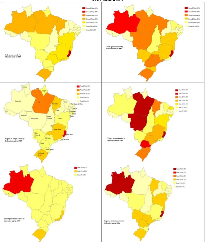
A detailed picture of trade patterns by Brazilian federal units in 1989 and 2004 is given in Figure 4. The values reveal large spatial inequalities with a high level of trade exposure in some Brazilian states.27 Although trade openness increased in each state in the period under study, disparities between the different federal units also grew: the “average” level of trade openness for the 26 states rose from 8% to 19.6% (standard deviations being 0.07 and 0.16 respectively). In 2004, trade openness ratios ranged from 0.9% in Acre (a state covered mostly by the Amazon jungle) to 44.8% in Amazonas (whose main economic activities are concentrated in the free-export zone of Manaus) and 59.9% in Espírito Santo (a coastal state that comprises some of the country’s main ports). A further six Brazilian states posted openness ratios above 30%.28

<Figure 4>

Figure 4 also maps the Brazilian states’ levels of export exposure and import penetration in 1989 and 2004. Some Brazilian states exhibit a very sharp rise in export-to-output ratios over this period. In 1989, only five states posted export exposure above 10% as opposed to twelve states in 2004, with four states above 25%: Espírito Santo and Pará (two states in which exports of iron ore play a major role) and Mato Grosso and Paraná (where soybean exports are very high).

More modest growth is found in import penetration: in 1989, ratios were below 5% in all the Brazilian states except Amazonas, Rio de Janeiro, Espírito Santo and Rio Grande do Sul. In 2004, only eight states had ratios above 10%, with Amazonas and Espirito Santo posting levels above 25%. In line with the observation for Brazil as a whole, it is mainly growth in exports that accounts for the increase in trade openness in the different federal units.

Note that an important feature of the Brazilian case is its strong geographical concentration of exports and imports. In 2004, three states29 accounted for more than 50% of total Brazilian exports while 20 states had less than a 5% share of total exports. The geographical concentration of imports is even more important, even though it has fallen since 1989: whereas 21 states had less than a 5% share of total imports in 2004, three states30 accounted for over 60% of total Brazilian imports.

From this analysis, it follows that integration into world markets was very uneven across the different federal units at the end of the 1980s and that these regional inequalities in terms of trade exposure have increased over the last two decades. This variation in Brazilian trade patterns across space and time may well play a role in the different state inequality and poverty trends.

Figures 5a and 5b show respectively the evolution of two of the most common indicators of inequality and poverty, the Gini index and the headcount ratio.The trends are presented for Brazil as a whole and separately for rural and urban areas from 1987 to 2005. The Gini index reveals a steady increase in inequality from 1987 to 1989 (with a peak at 0.63), followed by a certain amount of volatility through to 1993. Usual explanations for this trend include high and accelerating inflation over the period, as well as increasing levels of education among the population tied in with rising returns to schooling (see Ferreira and Paes de Barros, 2004). From 1993 to 2005, there was an initially slow but steady downturn in inequality (from 0.60 in 1993 to 0.56 by 2005). This reduction was sharper in rural areas than in urban zones and particularly significant from 2001 onwards. We observe a similar pattern in poverty indicators for the same period. The headcount ratio displays fluctuating values from 1987 to 1993, again reflecting macroeconomic instability and hyperinflation. From 1993 to 1995, a fall is observed in the poverty headcount. The introduction of the Social Assistance bylaw in 1993, which consisted essentially of unconditional cash transfers to poor aged people living in rural areas and to disabled persons, together with the Real Plan in 1994, are usually identified as

contributors to this initial poverty reduction (Ferreira et al., 2006; Pero and Szerman, 2009). A period of relative stability in the percentage of poor at around 33% followed from 1995 to 2003 (though poverty ratios in rural areas continued a slow, steady downturn). Finally, a persistent and significant drop in poverty ratios took place from 2003 onwards, this time both in urban and rural areas (the headcount index standing at 29% for Brazil in 2005).31

<Figures 5a and 5b>

Turning to the spatial aspect, when we look at the 1987-2005 period of analysis, there are considerable inequality and poverty differences not only across rural and urban areas but also across Brazilian states, in terms of both levels and trends. Figure 6a and Figure 6b show the first and last year Gini coefficients and headcount ratios in the Brazilian states. Although inequality fell in almost all federal units32, the intensity of the drop varied across states. Similar spatial heterogeneity is observed when looking at poverty levels. In fact, no convergence across states seems to have taken place during the timeframe of analysis.

<Figures 6a and 6b>

This paper sets out to investigate whether the rich spatial variation in welfare outcomes and trends observed in Brazil is linked to the variations observed in Brazilian states’ trade exposure. Our estimation strategy and results are described in the next section.

4. Impact of trade liberalization on inequality and poverty

4.a. Econometric specification.

To empirically estimate the effect of trade liberalization on inequality and poverty at state level (or rural and urban area level within states), our main econometric specification takes the form:

st t s i i ist st st

TradeLib

X

y

=

θ

+

∑

β

+

λ

+

γ

+

ε

where

y

Theil indices to capture inequality and the headcount ratio and poverty gap indices to capture poverty levels.

In this study, TradeLibst is the key variable and we use two measures for it: a measure based on

trade policy (our LIB indicator described above) and trade flow-based indicators (lagged import penetration, lagged export exposure and lagged trade openness). All these indicators represent different ways of capturing the extent of trade exposure across Brazilian states. Hence,

θ

Vector Xist includes i control variables typically assumed to affect levels of poverty and inequality.

Our main specification includes as controls: the share of individuals declaring themselves “white” in each state (to account for ethnic inequalities); the share of individuals by different levels of education in each state (to cover the role of educational inequalities), the share of informal workers in each state and the size of the agricultural sector in each state (both well-known determinants of the income distribution). Finally,

λ

ε

error term.

This paper draws on regional data to seek to answer the question of the impact of trade liberalization on regional outcomes, or more precisely within states. An underlying assumption in this type of analysis is that labor should not be too mobile across states in Brazil, at least in the short or medium run (there would be no differential effects across the country if wages, and consequently household income levels, were equalized across regions). However, as emphasized by Goldberg and Pavcnik (2007, p.56), “Failure of this premise to hold in practice does not invalidate the approach; it simply implies that one would not find any differential trade policy effects across industries/regions in this case”. In the case of Brazil, even though geographic migration is not inconsiderable throughout the period of study, it is not sizeable enough to wipe out the spatial disparities in the experiences observed.33

4.b. Empirical findings

The estimated effects of our trade policy indicator LIB on poverty are presented in Table 1a. The table reports on equation (1), estimated using both the headcount ratio and the poverty gap index as poverty indicators. For each dependent variable, results are reported using the state as a whole as the unit of analysis (columns 1 and 4). However, since rural and urban areas within states may be very different, we also examine equation (1) separately for urban areas (columns 2 and 5) and rural areas (columns 3 and 6) within states.

Table 1a reveals a negative effect of our trade policy indicator LIB on poverty when we look at the state level (columns 1 and 4), although this is only statistically significant when poverty is measured by the poverty gap (and only significant at 10%). This means that, at the state level, trade liberalization might have contributed to poverty increases. In other words, even if Brazilian states on the whole saw a fall in poverty over the period studied, the Brazilian states more affected by tariff reductions posted smaller reductions in poverty (at least in terms of the poverty gap index). Our estimation suggests that, on average, a decrease of one percentage point in the trade policy indicator LIB would lead to an increase in the poverty gap of 0.16 percentage point.

The fact that rural and urban areas within states are very different may be behind our low significance levels when the state as a whole is used as the unit of analysis. In fact, if we concentrate on urban areas only (columns 2 and 5), the negative effect of trade liberalization on poverty is highly significant and the size of our trade policy indicator LIB coefficients is also larger, regardless of the poverty measure used. On average, a fall of one percentage point in the trade policy indicator LIB in urban areas of states would lead to a 0.67 percentage point increase in the headcount ratio, and a 0.23 percentage point increase in the poverty gap. On the other hand, no significant effect is observed in rural areas (columns 3 and 6).

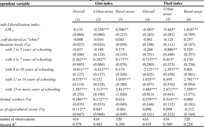
In the estimation of equation (1) we include a few control variables considered to be usual determinants of poverty and inequality. Concerning our poverty results in Table 1a, controls are almost all highly significant and have the expected signs. Education is almost always significant and reduces poverty at practically all levels of education, while an increase in the share of informal workers leads to a significant rise in poverty. The size of the agricultural sector in a state matters: it leads to a significant rise in poverty.34 As expected, informal jobs and agricultural employment show

up as significant determinants of poverty. The share of individuals declaring themselves to be “white” is never significant.

<Tables 1a and 1b>

Table 1b presents the relationship between trade liberalization and inequality. When we consider the state as a whole as the unit of analysis (columns 1 and 4), our trade policy indicator LIB is inequality increasing, but the effect is again only significant using one inequality measure, the Theil index (more sensitive than the Gini coefficient to changes in the tails of the distribution). In other words, Brazilian states that were more affected by tariff cuts experienced smaller reductions in inequality (at least in terms of the Theil index). However, opposing and significant patterns emerge when we consider urban and rural areas separately, these patterns being robust to the choice of inequality measure. The influence of a tariff reduction is inequality increasing in urban areas (columns 2 and 5) and inequality decreasing in rural zones (columns 3 and 6).35

One tentative explanation for our contrasting effects of trade liberalization on household poverty and inequality between urban and rural areas could be that urban workers – essentially employed in the manufacturing industries and in the service sector – suffered the most from the liberalization process. Previous research on Brazil has established that trade liberalization led to a downturn in economy-wide wage inequality (Gonzaga et al., 2006; Ferreira et al., 2007a). At the same time, recent evidence on labor reallocations in response to trade reforms in Menezes and Muendler (2007) shows labor displacements from import competing industries in the 1990s, but neither comparative-advantage industries nor exporters seem to have absorbed trade-displaced workers for years. Indeed, more frequent transitions to informal work status and unemployment are observed. These transitions may be sources of poverty and inequality increases and these effects are captured when total household income (not just wages) is considered. Should these adjustments play a relatively greater role in urban areas than other inequality-decreasing mechanisms, they could well be behind our poverty- and inequality-increasing findings in urban areas, and could also help explain the differences between rural and urban results. Although this is beyond the scope of this paper, our results suggest that a better understanding of the effects of trade liberalization on household income distribution should take into

account not only the observed changes in labor income, but also whether there have been any trade-induced changes in household composition and in the occupational status of all household members.36

Note also that trade liberalization was more intense in the manufacturing sectors, with major tariff reductions taking place from 1990 onwards (see section 2). In the agricultural sectors, there was less reduction in protection from 1990 onwards and Brazil has strong comparative advantages in these sectors, where an important rise in exports has occurred (see subsection 4.b.ii).37 So when only rural areas within states are considered, it is not surprising to find that trade liberalization has no significant effects on poverty and even to find levels of inequality reduced if anything.

Another reason for observed differences in the results on poverty and inequality across urban and rural areas may be related to a differential role of social transfers. In particular, given the major role of conditional cash transfer programs in poverty reduction, we were concerned that if these transfers were correlated with exposure to trade, their omission would result in an omitted variable bias. Unfortunately, our data cannot identify individuals’ income sources (and more specifically transfers received) for the entire period of analysis nor can we capture federal expenditures by state.38 But we do know that conditional cash transfer programs were initially implemented in a few municipalities to be rolled out nationwide in 2001 (essentially with the introduction of the Bolsa Escola and Bolsa Alimentação programs, then unified and scaled up in the Bolsa Familia program in 2003). We decided to rerun our regressions excluding the 2001-2005 period and our results are still robust. Although the size of our trade liberalization coefficient falls some 30% on average in the poverty and inequality regressions, we still observe opposing and significant effects across urban and rural areas within states.

To sum up, our results show that trade liberalization, as measured by our LIB indicator, raises poverty and inequality in Brazilian states, although these effects are mildly significant. The distinction between rural and urban areas gives more insight into the effect of trade liberalization. In urban areas, we observe a negative and always significant effect for both poverty and inequality. In rural zones, the sign of the effect of trade liberalization is reversed (although significant only when looking at inequality). Our findings for state poverty are in line with recent results for Indian districts (Topalova, 2005), even though no parallel significant effect on inequality is found in India. However, the poverty increase due to trade liberalization observed in India occurs in the rural world, while it appears to

occur in urban areas in Brazil. Whereas, in the case of India, sectors that have been relatively more affected by tariff reductions are concentrated in rural districts, descriptive evidence for Brazil (Figure 2) shows that trade liberalization was more intense in manufacturing sectors, typically set up in urban zones.

We have investigated whether these results are robust to the choice of trade liberalization indicator. In our trade policy measure LIB, tariffs are weighted by the number of workers in each industry as a share of total employment in each state. Some authors (Topalova, 2005; Edmonds et al., 2007) raise the question of considering employment only in “tariff-protected” industries. Therefore, an alternative

LIB2 indicator is also constructed where the employment shares are calculated for employment solely

in “tariff-protected” industries, i.e.:

) ( ) ( 2 1987 1987

∑

∑

where s stands for the unit of analysis, k for the sector and t for time.

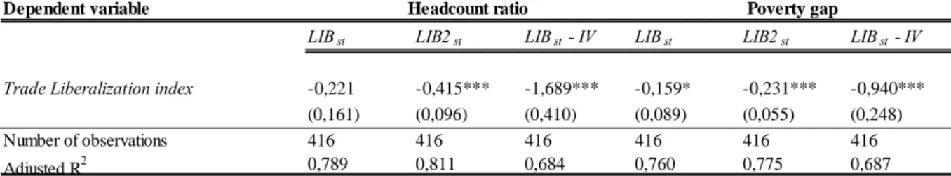
A problem with LIB2 is that it does not reflect the size of the traded sector within a state. Consider two states with the same structure of employment in “tariff-protected” industries; the indicator will now inevitably have the same value across the two states even if the shares of workers in “tariff-protected” industries as a proportion of total employment are very different. As a consequence, the magnitude of trade policy effects may by construction be overstated by LIB2. To overcome this problem, another estimation strategy is implemented, the instrumentation of LIB by LIB2. In both cases, we obtain similar trade policy effects on our income distribution variables at state level: when significant, the effect of trade liberalization is poverty and inequality increasing (see tables A2 and A3 in the appendix).

Additional robustness checks have been performed. In particular, we have estimated regressions excluding states that can be considered to be outliers, like Distrito Federal and Amazonas. On the one hand, Distrito Federal (Brasília) has a very peculiar productive, labor and revenue pattern compared with the rest of the country. It is a fundamentally administrative city in which the majority of national government activities are concentrated. Amazonas, on the other hand and as pointed out earlier, benefits from special trade regimes because of the “free trade zone” status held by the Manaus

industrial area. As regards poverty, a different poverty line of R$75 was also tested. In all cases, our main results hold.39

4.b.ii. International trade, poverty and inequality

Brazil is one of the few countries in which international trade flows can be observed and measured by federal units, and where the number of units of analysis allows exceptionally for the use of a regression framework to study the effects of trade openness, import penetration and export exposure on state poverty and inequality. These indicators reflect the degree of integration of Brazilian states into world markets. Note that they differ from our LIB measure based on tariff cuts. They are not exclusively influenced by trade policies, as trade flows are also determined by other factors such as transport costs, macroeconomic policies, factor endowments, the country’s size and geographical situation, etc. Our dataset allows us to distinguish between the effects of imports and exports on poverty and inequality. In the end, the combination of data on tariffs as well as on imports and exports at a subnational level, allows for an all-embracing appraisal of the distributional impacts of trade. The responses of poverty and inequality indices to our trade flow-based measures are documented in Tables 2a and 2b respectively. Given that no separate data are available on trade flows in rural and urban areas within states, we can only provide evidence using the state as a whole as the unit of analysis. However, in an effort to study the influence of trade integration on poverty and inequality at a more disaggregated level, we have constructed import and export ratios separately for agricultural and industrial sectors.

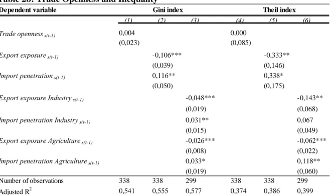
Table 2a presents the results on poverty incidence (columns 1, 2 and 3) and poverty depth (columns 4, 5 and 6). For each poverty measure, three specifications are tested to capture the effect of international trade: (i) the inclusion of a measure of lagged trade openness; (ii) the inclusion of lagged import penetration and lagged export exposure ratios simultaneously and (iii) the inclusion of lagged import penetration and lagged export exposure ratios separately for agricultural and industrial sectors A similar specification structure is used in Table 2b to capture the impact of international trade on

both Gini and Theil inequality measures. For the sake of simplicity, control variables included in the regressions are not reported, though available on request.

<Tables 2a and 2b>

Two noteworthy results emerge. First, for both poverty and inequality, trade openness has no significant impact regardless of the income distribution measure used (see the coefficient for the Trade

opennesss(t-1) variable in columns 1 and 4 of tables 2a and 2b). However, a different picture emerges

when we look into the separate influence of export exposure and import penetration (see the coefficients for the Export exposures(t-1) and Import penetrations(t-1) variables in columns 2 and 5 of

tables 2a and 2b): the rise in export exposure appears to reduce poverty and inequality quite significantly while import penetration growth increases both income distribution measures. If we evaluate the magnitude of the coefficients, we see from column 2 in Table 2a that a one percentage point rise in import penetration in a state leads to a 0.23 percentage point increase in poverty incidence (significance is lost for our poverty depth measure in column 5). For export exposure, a one percentage point rise leads, on the contrary, to a 0.12 fall in poverty based on the headcount ratio (-0.07 with the poverty gap). As regards inequality, a one percentage point rise in import penetration raises the Gini coefficient by 0.12 (0.34 for the Theil index), while a one percentage point rise in export exposure decreases the Gini coefficient by -0.11 (-0.33 in the Theil index).

To sum up, we see that import penetration yields results consistent with our findings regarding the trade policy-based measure: a rise in the import penetration ratio increases poverty incidence and inequality at state level. At the same time, tariff cuts -when significant- are also related to rising poverty and inequality levels at state level. Conversely, trade integration via rising export ratios clearly contributes to a fall in poverty and inequality.

In Brazil, agricultural exports have enjoyed sharp growth (551% between 1989 and 2004 in current dollars), much higher than the increase in industrial exports (168% over the same period). However, agricultural imports have grown less than industrial imports (36% as opposed to 268%).40 Concerning trade intensity, export exposure and import penetration ratios in 2004 were considerably stronger for industry (the state’s average export exposure ratios for industry and agriculture were respectively 32.4 and 8.5 in 2004; in turn, the state’s average import penetration ratios stood at 37.9 and 22.8). To see if

there are any differential effects on the income distribution measures depending on the sector concerned, columns 3 and 6 of tables 2a and 2b present the effects of international trade on poverty and inequality when export and import ratios are constructed separately for the agricultural and industrial sectors (the latter including mining industries).

Our results find, once more, an opposite sign for export exposure and import penetration effects on welfare for both industry and agriculture. In both the industrial sector and the agricultural sector, growth in export exposure reduces poverty and inequality while the rise in import penetration (when significant) increases both welfare measures. No clear differential effect is observed between the industrial and agricultural sectors in terms of the impact of trade exposure on poverty and inequality.

4.b.iii. The effect of trade exposure on income distribution: quintile analysis

When summary inequality measures such as the Gini or the Theil index are used, we cannot easily tell where in the income distribution variations are occurring. In an effort to better grasp how trade liberalization affects the shape of the entire income distribution in each state, instead of just focusing on summary poverty and inequality statistics, we have also calculated income levels for each quintile (and also decile) in each state s at time t, and have run the additional set of equations:

st t s i ist i st stj

TradeLib

X

y

=

θ

+

∑

β

+

λ

+

γ

+

ε

where

y

state s at time period t.

<Table 3>

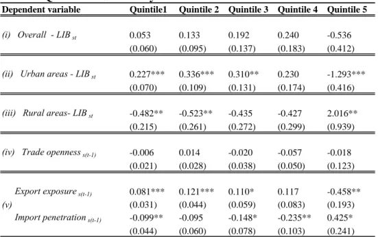
Table 3 presents a summary of all our estimations of equation (2) for each quintile where only the values and standard errors of the coefficients on our variables of interest are reported, that is: (i) on our trade policy indicator LIB using the entire state as the unit of analysis; (ii) then considering only urban areas within states; (iii) and only rural areas within states; (iv) on our indicator of lagged trade openness; (v) and finally on our measures of lagged import penetration and export exposure ratios simultaneously included in the regression. 41

Although no significant effect is found for trade policy measure LIB at state level, no matter which quintile regression is considered, there is evidence of growing (falling) inequality in urban (rural) areas linked to trade liberalization: this comes from the coefficients sharing a similar positive (negative) sign in all quintiles except the highest one, where the sign is reversed. Distributional changes due to trade liberalization are therefore observed along the income ladder (and are particularly significant for the first, second and fifth quintiles). As regards our trade flow-based variables, the quintile regressions again find no significant effect of trade openness. However, export exposure increases the relative income levels of all quintiles except the last one, which presents the opposite sign, while import penetration increases the relative income levels of the upper quintile and decreases the relative income levels of the other quintiles (these effects are significant for almost all quintile levels). An interesting fact arises in Table 4 from an examination of coefficient sizes by quintile. Regardless of the variable chosen to measure trade exposure and the levels of disaggregation in the state population (entire state, or urban or rural areas within states), the impact on the quintiles’ relative income levels is non-monotonic. The second quintile group’s coefficients are systematically larger than those of the first quintile counterpart, but not necessarily lower than those of the third or fourth quintile. In a sense, the effects of exposure to trade, though fully shared across the entire length of the income ladder, seem relatively weaker among the poorest of the poor and intermediate (third and fourth) quintile groups. The fact that the poorest of the poor are less affected than those households closer to the poverty line is suggested by the findings of our two poverty measures in previous regressions. Looking at the effects of our trade liberalization variables on poverty incidence and poverty depth (Table 1a), the coefficients are systematically lower in the second case (last three columns versus first three columns) when distance to the poverty line is taken into account.

5. Conclusion

Brazil has undergone an extensive trade liberalization reform since 1988, which has significantly changed the economy’s level of protection. Since the 1990s, Brazil has also posted a slow but significant downturn in both poverty and inequality indicators, although high levels of inequality and

persistent poverty remain, with considerable geographic differences. Can we establish a causal link between changes in trade policies and international trade flows and changes in poverty and inequality across regions in Brazil over the last two decades? Is this effect different in rural and urban areas?

This paper draws on various data sources to quantify the impact of trade liberalization and international trade on household income inequality and poverty across Brazilian states from 1987 to 2005. In particular, we measure whether states more exposed to trade posted relatively smaller or larger changes in household poverty and inequality than less exposed states. Our main contributions to the literature are threefold. First, by using sub-national units of observation (in our case, Brazilian states together with the distinction between rural and urban areas within states), this paper adds to the recent literature that includes a spatial dimension in the study of trade liberalization effects on income distribution. Second, the availability of long household survey series of remarkable quality allows for various measures of household poverty and inequality at state level to be calculated. This means that the analysis can include how trade affects not only workers, but also their dependents and people involved in non-traded sectors. Last but not least, it is one of the few studies to consider both trade policy variables and international trade flow variables (at the sector level) in an effort to be exhaustive in its assessment of the distributional impacts of trade.

Our results show that, regardless of the nationwide effects of trade liberalization, states more exposed to tariff cuts (i.e. with a greater share of workers in industries with initially high tariffs) posted smaller reductions in household poverty and inequality. Although the significance of the results for the states as a whole appears to be dependent on the choice of poverty and inequality indicators, this is not the case when the states are disaggregated into rural and urban areas. Indeed significant and opposing effects emerge. Urban areas more affected by trade liberalization experienced lower poverty and inequality reductions (on average, a fall of one percentage point in our trade liberalization indicator in urban areas raises the headcount ratio by 0.67 percentage points and the Gini index by 0.26 percentage points). In the rural world, trade liberalization seems to have been inequality decreasing (Gini index increasing by 0.51 percentage points) and no significant effect on poverty is observed. These results are non-negligible and are confirmed by several robustness checks.

Tariff cuts are only one aspect of trade openness. To better gauge integration into world markets, international trade flow data are exceptionally available at the state level in the case of Brazil. When measures based on international trade flows are considered, our results find significant and opposite effects for import penetration and export exposure ratios. A rise in the export exposure of Brazilian states appears to reduce poverty and inequality quite significantly while growth in import penetration increases both income distribution measures at state level – this latter result is in line with the finding for tariff reductions. These effects are still observed when we consider trade flows separately in the industrial and agricultural sectors. As rising export ratios have a positive effect on welfare outcomes, the reduction in poverty and inequality in Brazil might be bolstered by the recent Brazilian trade performance. Indeed, Brazil has been posting a trade surplus since 2002 and sharp growth in exports in recent years.

Finally, and although beyond the scope of this paper, our differential effects across urban and rural areas in Brazil should encourage further research on the various trade transmission channels in operation for household income distribution, which may work differently depending on geographic location. The role of trade-induced changes in labor income, but also in household composition and occupational status of all household members could well differ across regions.

6. References

Attanasio O., Goldberg P., Pavcnik N., 2004 “Trade Reforms and Wage Inequality in Colombia”, Journal of Development Economics 74, pp. 331-366.

Abreu, M. P., 2004, Trade liberalization and the political economy of protection in Brazil since 1987. INTAL-ITD Working Paper SITI 08B. Inter-American Developing Bank, Buenos Aires.

Arbache, J., Dickerson, A., Green, F., 2004, Trade Liberalisation and Wages in Developing Countries", The Economic Journal, 114 (February), pp. F73–F96.

Bethell, L. (ed.), 2001, História da América Latina - A América Latina Após 1930: Economia e Sociedade. Volume VI. Edusp, São Paulo.

Bourguignon, F., Ferreira, F., Lustig, N., 2004. The Microeconomics of Income Distribution Dynamics in East Asia and Latin America, The World Bank and Oxford University Press, Washington DC.

Carvalho, A., De Negri, J.A., 2000, Estimação de equações de importação e exportação de produtos agropecuários para o Brasil (1977/1998), Texto para Discussão 698, Instituto de Pesquisas Aplicadas (IPEA), Brasília.

Carvalho Jr., M. C., 1992, Alguns aspectos da reforma aduaneira recente, Texto para Discussão 74, Fundação Centro de Estudos do Comércio Exterior, Rio de Janeiro.

Cogneau, D., Gignoux, J., 2009, Earnings Inequalities and Educational Mobility in Brazil over Two Decades, in: Klasen S., F. Nowak-Lehman (eds), Poverty, Inequality and Policy in Latin America, MIT Press, CESifo Seminar Series, Cambridge MA.

Corseuil, C.H.L., M.N. Foguel, 2002, Uma Sugestão de Deflatores para Rendas Obtidas a partir de Algumas Pesquisas Domiciliares do IBGE, Texto para Discussão 897, Instituto de Pesquisas Aplicadas (IPEA), Rio de Janeiro.

Edmonds E. V., Pavcnik, N., Topalova, P., 2007, Trade Adjustment and Human Capital Investments: Evidence from Indian Tariff Reform, IMF Working Paper WP/07/94, International Monetary Fund, Washington DC.

Fally T., Paillacar R., Terra C., 2008, Economic Geography and Wages in Brazil: Evidence from Micro-Data, Thema Working Paper 2008-23, University of Cergy-Pontoise: Cergy-Pontoise. Ferreira, F., Paes de Barros, R., 2004, The Slippery Slope: Explaining the Increase in Extreme Poverty

in Urban Brazil, 1976-96, in: Bourguignon, F., Ferreira, F. et Lustig, N. (Eds.), The Microeconomics of income distribution dynamics in East Asia and Latin America, The World Bank, Washington DC.

Ferreira F. H.G., Leite P.G., and Wai-Poi M., 2007a, Trade Liberalization, Employment Flows and Wage Inequality in Brazil, World Bank Policy Research Working Paper 4108, The World Bank, Washington DC.

Ferreira F. H.G., Leite P.G., and Ravallion M., 2007b, Poverty Reduction Without Economic Growth? Explaining Brazil’s Poverty Dynamics, 1985-2004, World Bank Policy Research Working Paper 4431,The World Bank, Washington DC.

Ferreira F. H.G., Leite P., Litchfield J., 2006, The Rise and Fall of Brazilian Inequality: 1981-2004, World Bank Policy Research Working Paper 3867, The World Bank, Washington DC.

Fiess, N.M., Verner, D., 2003, Migration and Human Capital in Brazil during the 1990s, World Bank Policy Research Working Paper 3093, The World Bank, Washington DC.

Gonzaga G., Menezes Filho N., Terra M.C., 2006, Trade Liberalization and the Evolution of Skill Earnings Differentials in Brazil, Journal of International Economics 68/2, pp. 345-367.

Goldberg P. K., Pavcnik N., 2007 Distributional Effects of Globalization in Developing Countries, Journal of Economic Literature XLV (March), pp. 39–82.

Goldberg P. K., Pavcnik N., 2005 Trade, wages, and the political economy of trade reform: Evidence from the Colombian trade reform, Journal of International Economics, 66 (1), May, pp. 75-105.

Goldberg P. K., Pavcnik N., 2004, Trade, Inequality, and Poverty: What Do We Know? Evidence from Recent Trade Liberalization Episodes in Developing Countries, NBER Working Paper

Series 10593, National Bureau of Economic Research, Massachusetts.

Hanson, G.H., 2005, Market potential, increasing returns, and geographic concentration, Journal of International Economics 67(1), pp. 1-24.

Hanson G.H., 2003, What Has Happened to Wages in Mexico since NAFTA? Implications for Hemispheric Free Trade, NBER Working Paper Series 9563, National Bureau of Economic Research, Massachusetts.

Harrison, A. (ed.), 2007, Globalization and Poverty, NBER, The University of Chicago Press.

Kume, H., Piani, G., Souza, C.F., 2003, A Politica Brasileira de Importacão no Periodo 1987-98: Descricão e Avaliação, in: Corseuil, C.H., Kume, H. (eds.), A Abertura Comercial nos Anos 1990 – Impactos Sobre Emprego e Salário, Ministério do Trabalho e Emprego and IPEA, Rio de Janeiro, pp. 9-37.

McCaig, B., 2009, Exporting Out of Poverty: Provincial Poverty in Vietnam and U.S. Market Access, Working Paper in Economics & Econometrics 502, Australian National University, Canberra. Menezes Filho, N.A., Muendler, M.A., 2007, Labor Reallocation in Response to Trade Reform,

CESifo Working Paper 1936, CESifo, Munich.

Nicita, A., 2004, Who benefited from trade liberalization in Mexico? Measuring the effects on household welfare, World Bank Policy Research Working Paper Series 3265, The World Bank, Washington D.C.

Paes de Barros, R., Foguel, M. N., Ulyssea, G., 2006, Desigualdade de renda no Brasil: uma análise da queda recente, Instituto de Pesquisas Aplicadas (IPEA), Rio de Janeiro

Pavcnik, N., Blom A., Goldberg P. K. et Schady N., 2004, Trade policy and Industry Wage Structure: Evidence from Brazil, World Bank Economic Review 18 (3), pp. 319–44.

Pavcnik, N., Blom, A., Goldberg, P., Schady, N., 2003,Trade Liberalization and Labor Market Adjustment in Brazil, World Bank Policy Research Working Paper 2982, The World Bank, Washington D.C.

Pereira, L. V., 2006, Brazil Trade Liberalization Program, In: Córdoba, S., Sam Laird. (Eds.) Coping with Trade Reforms: A Developing-Country Perspective on the WTO Industrial Negotiations. Palgrave MacMillan, Houndmills and New York.

Pero, V., Szerman, D., 2009, The new generation of social programs in Brazil, Instituto de Economia, Universidade Federal do Rio de Janeiro, mimeo.

Porto G., 2006, Using Survey Data to Assess the Distributional Effects of Trade Policy, Journal of International Economics 70, pp. 140-160.

Porto G., 2003, Trade Reforms, Market Access, and Poverty in Argentina, World Bank Policy Research Working Paper 3135, The World Bank, Washington DC..

Pourchet, H. C. P., 2003, Estimação de equações de exportação por setores: uma investigação do impacto do câmbio, Dissertação (MSc.), Pontifícia Universidade Católica do Rio de Janeiro, Rio de Janeiro.

Redding S., Venables A.J., 2004, Economic geography and international inequality, Journal of International Economics 62(1), pp. 53-82.

Ribeiro, L. S., 2006, Dois ensaios sobre a balança comercial brasileira: 1999-2005, Dissertação (MSc.), Pontifícia Universidade Católica do Rio de Janeiro, Rio de Janeiro.

Robbins, D., 1996, Evidence on trade and wages in the developing world, OECD Technical Paper 119, OECD, Paris.

Topalova P., 2005, Trade Liberalization, Poverty and Inequality: Evidence from Indian Districts, NBER Working Paper Series 11614, National Bureau of Economic Research, Massachusetts.. Wei S., Y. Wu, 2002, Globalization and Inequality Without Differences in Data Definitions, Legal

System, and Other Institutions, International Monetary Fund, mimeo.

Winters A. L., McCulloch N., A. McKay, 2004, Trade Liberalization and Poverty: The Evidence So Far, Journal of Economic Literature XLII, pp. 72-115.