HAL Id: pastel-00006121
https://pastel.archives-ouvertes.fr/pastel-00006121
Submitted on 3 Jun 2010HAL is a multi-disciplinary open access
archive for the deposit and dissemination of sci-entific research documents, whether they are pub-lished or not. The documents may come from teaching and research institutions in France or abroad, or from public or private research centers.
L’archive ouverte pluridisciplinaire HAL, est destinée au dépôt et à la diffusion de documents scientifiques de niveau recherche, publiés ou non, émanant des établissements d’enseignement et de recherche français ou étrangers, des laboratoires publics ou privés.
L’alignement de graphes : applications en
bioinformatique et vision par ordinateur
Mikhail Zaslavskiy
To cite this version:
Mikhail Zaslavskiy. L’alignement de graphes : applications en bioinformatique et vision par ordinateur. Mathématiques [math]. École Nationale Supérieure des Mines de Paris, 2010. Français. �pastel-00006121�
T
H
È
S
E
INSTITUT DES SCIENCES ET TECHNOLOGIES
´
Ecole doctorale nO431 : Information, Communication, Mod´elisation et Simulation
Doctorat ParisTech
T H `
E S E
pour obtenir le grade de docteur d´elivr´e par
l’´
Ecole nationale sup´
erieure des mines de Paris
Sp´
ecialit´
e ”Bioinformatique”
pr´esent´ee et soutenue publiquement par
Mikhail Zaslavskiy
le 11 Janvier 2010
Graph matching and its application in computer
vision and bioinformatics
Directeurs de th`ese: Francis BACH and Jean-Philippe VERT
Jury:
Colin DE LA HIGUERA
Pr´esident
Martial HEBERT
rapporteur
Benno SCHWIKOWSKI
rapporteur
Nicola CANCEDDA
examinateur
Francis BACH
examinateur
Jean-Philippe VERT
examinateur
MINES ParisTech CBIO & CMM 35 rue Saint-Honor´e, Fontainebleau
R´
esum´
e
Le probl`eme d’alignement de graphes, qui joue un rˆole central dans diff´erents domaines de la reconnaissance de formes, est l’un des plus grands d´efis dans le traitement de graphes. Nous proposons une m´ethode approximative pour l’alignement de graphes ´etiquet´es et pond´er´es, bas´ee sur la programmation convexe concave. Une applica-tion importante du probl`eme d’alignement de graphes est l’alignement de r´eseaux d’interactions de prot´eines, qui joue un rˆole central pour la recherche de voies de signalisation conserv´ees dans l’´evolution, de complexes prot´eiques conserv´es entre les esp`eces, et pour l’identification d’orthologues fonctionnels. Nous reformulons le probl`eme d’alignement de r´eseaux d’interactions comme un probl`eme d’alignement de graphes, et ´etudions comment les algorithmes existants d’alignement de graphes peuvent ˆetre utilis´es pour le r´esoudre.
Dans la formulation classique de probl`eme d’alignement de graphes, seules les correspondances bijectives entre les noeuds de deux graphes sont consid´er´ees. Dans beaucoup d’applications, cependant, il est plus int´eressant de consid´erer les corre-spondances entre des ensembles de noeuds. Nous proposons une nouvelle formulation de ce probl`eme comme un probl`eme d’optimisation discret, ainsi qu’un algorithme approximatif bas´e sur une relaxation continue.
Nous pr´esentons ´egalement deux r´esultats ind´ependents dans les domaines de la traduction automatique statistique et de la bio-informatique. Nous montrons d’une part comment le probl`eme de la traduction statistique bas´e sur les phrases peut ˆetre reformul´e comme un probl`eme du voyageur de commerce. Nous proposons d’autre part une nouvelle mesure de similarit´e entre les sites de fixation de prot´eines, bas´ee sur la comparaison 3D de nuages atomiques.
Abstract
The graph matching problem is among the most important challenges of graph pro-cessing, and plays a central role in various fields of pattern recognition. We propose an approximate method for labeled weighted graph matching, based on a convex-concave programming approach which can be applied to the matching of large sized graphs. This method allows to easily integrate information on graph label similari-ties into the optimization problem, and therefore to perform labeled weighted graph matching. One of the interesting applications of the graph matching problem is the alignment of protein-protein interaction networks. This problem is important when investigating evolutionary conserved pathways or protein complexes across species, and to help in the identification of functional orthologs through the detection of con-served interactions. We reformulate PPI alignment as a graph matching problem, and study how state-of-the-art graph matching algorithms can be used for this purpose.
In the classical formulation of graph matching, only one-to-one correspondences are considered, which is not always appropriate. In many applications, it is more interesting to consider many-to-many correspondences between graph vertices. We propose a reformulation of the many-to-many graph matching problem as a discrete optimization problem and we propose an approximate algorithm based on a contin-uous relaxation.
In this thesis, we also present two interesting results in statistical machine lation and bioinformatics. We show how the phrase-based statistical machine trans-lation decoding problem can be reformulated as a Traveling Salesman Problem. We also propose a new protein binding pocket similarity measure based on a comparison of 3D atom clouds.
Acknowledgments
First of all, I would like to thank my scientific advisors Jean-Philippe Vert and Francis Bach. I think that it was a great piece of luck that I met them four years ago. I admire their way of guiding Phd students, they somehow manage to keep an optimal ratio between student research freedom and the value of their research, making sure that students spend their time usefully. It was always very easy for me to get their advice and meet them in person, when I needed it. At the same time, they always kept an eye on me, directing my research efforts in the right direction and encouraging my work. I have very happy memories of the exchange of emails the nights before deadlines, of long discussions with Jean-Philippe, when he asked me sequences of questions and helped me to answer them in order to make me solve yet another problem “by myself”, of brainstormings with Francis in front of a blackboard where he guided me in the construction of more and more interesting convex relaxations. Thank you very much for all you have done for me !
I would also like to express my gratitude to all other members (former and current) of the Center for Computational Biology, Pierre, Martial, Laurent, Brice, Veronique, Fantine, Christian, Yoshi, Kevin, Isabelle, Nathalie, Anne-Claire, Franck, Toby, Philippe for their help, for many interesting discussions and a lot of happy times (“le cbio c’est bien !”).
I spent most of the time during my Phd at the campus of Mines ParisTech in Fontainbleau where I met a lot of good friends with whom I shared a lot of happy moments playing volleyball, football and waiting for the school bus, and I would like to thank them for this.
I would also like thank my colleagues from the laboratory U900 (Insitut Curie) 4
5 and from the Willow-team (ENS-INRIA) for many valuable discussions and their willingness to help me in my work.
During my Phd, I had the chance to spend three months at Xerox Research Center Europe in Grenoble, and I am profoundly grateful to Marc and Nicola for inviting me there and working with me. In spite of the very short time, we did an excellent job together. Many thanks to all other members of XRCE for a warm welcome, hiking in mountains and teaching me climbing.
My Phd defense would not be possible without my jury: Martial Hebert, Benno Schwikowski, Nicola Cancedda and Colin De La Higuera, thank you very much for being there and for your comments on my work.
Finally, I would like to thank my family for supporting me all these years, and especially Tanya for her tolerance towards my endless deadlines and keeping me always ready to do the research. The day before my Phd defense, she told me ”I am so happy that you will finally get you Phd” (by the way, it reminds me some stories from phdcomics.org). Now, I have it.
Contents
R´esum´e 2
Abstract 3
Acknowledgments 4
Introduction 13
1 The graph matching problem . . . 13
1.1 Contribution & Perspectives . . . 17
2 Phrase-based statistical machine translation . . . 20
2.1 Contribution & Perspectives . . . 22
3 Comparison of protein binding pockets . . . 23
3.1 Contribution & Perspectives . . . 23
4 Publications . . . 25
I
Graph matching
27
1 Introduction 28 1.1 Basic definitions and notations . . . 281.2 Formulation of the graph matching problem . . . 29
1.3 Alternative formulations of graph matching . . . 32
1.3.1 Vertex labels . . . 33
1.3.2 Quadratic assignment problem . . . 34
1.3.3 Matching graphs of different sizes . . . 35 6
CONTENTS 7
1.3.4 l1 and other alternatives to the l2 norm in the GM problem . . 37
1.3.5 Graph edit distance . . . 38
1.3.6 Complexity of the graph matching problem . . . 40
1.4 Early history of graph matching . . . 40
1.4.1 Recent developments in graph matching . . . 46
1.5 Applications of graph matching algorithms . . . 47
1.6 GM, kernels and graph invariants . . . 48
2 A path following algorithm for GM 50 2.1 Introduction . . . 52
2.2 Problem description . . . 54
2.2.1 Permutation matrices . . . 55
2.2.2 Approximate methods: existing works . . . 56
2.3 Convex-concave relaxation . . . 59
2.3.1 Convex relaxation . . . 60
2.3.2 Concave relaxation . . . 60
2.3.3 PATH algorithm . . . 63
2.3.4 Numerical continuation method interpretation . . . 66
2.3.5 Some implementation details . . . 68
2.3.6 Algorithm complexity . . . 72
2.3.7 Vertex pairwise similarities . . . 73
2.4 Simulations . . . 74
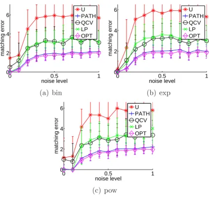
2.4.1 Synthetic examples . . . 74
2.4.2 Results . . . 75
2.5 QAP benchmark library . . . 79
2.6 Image processing . . . 81
2.6.1 Alignment of vessel images . . . 81
2.6.2 Recognition of handwritten chinese characters . . . 84
2.7 Conclusion . . . 86
2.A A toy example . . . 86
8 CONTENTS 3 Global alignment of PPI by GM methods 89
3.1 Introduction . . . 90
3.2 Constrained and balanced GNA problems . . . 92
3.3 Methods . . . 96
3.3.1 Algorithms for the balanced GNA problem . . . 96
3.3.2 Algorithms for the constrained GNA problem . . . 98
3.4 Data . . . 102
3.5 Results . . . 103
3.5.1 Disambiguation of functional orthologs within Inp. clusters . . 104
3.5.2 Disambiguation of Inp. clusters with second-order interactions 109 3.5.3 Global PPI network alignment . . . 111
3.6 Discussion . . . 113
4 Many-to-Many graph matching 116 4.1 Introduction . . . 116
4.2 Many-to-many graph matching as an optimization problem . . . 119
4.3 Continuous relaxations of the many-to-many GM problem . . . 122
4.3.1 Method 1: Gradient descent . . . 122
4.3.2 Method 2: SDP relaxation . . . 123
4.4 Related methods . . . 125
4.5 Experiments . . . 126
4.5.1 Synthetic examples . . . 126
4.5.2 Chinese characters . . . 128
4.5.3 Identification of object composite parts . . . 129
4.6 Conclusion . . . 131
II
Other applications
133
5 PBSMT as a Traveling Salesman Problem 134 1 Introduction . . . 135CONTENTS 9
3 The Traveling Salesman Problem and its variants . . . 138
3.1 Reductions AGTSP→ATSP→STSP . . . 139
3.2 TSP algorithms . . . 140
4 Phrase-based Decoding as TSP . . . 141
4.1 From Bigram to N-gram LM . . . 143
5 Experiments . . . 146
5.1 Monolingual word re-ordering . . . 146
5.2 Translation experiments with a bigram language model . . . . 147
6 Future Work . . . 151
7 Conclusion . . . 152
6 A new binding pocket similarity measure 154 1 Introduction . . . 155
2 Methods . . . 156
2.1 Convolution kernel between atom clouds . . . 156
2.2 Related methods . . . 160 2.3 Performance criteria . . . 162 2.4 Docking . . . 164 3 Datasets . . . 165 4 Results . . . 166 4.1 Kahraman Dataset . . . 167 4.2 Homogeneous dataset (HD) . . . 171 5 Discussion . . . 172
List of Tables
2.1 Experiment results for QAPLIB benchmark datasets. . . 80
2.2 Alignment of vessel images, algorithm performance . . . 82
2.3 Classification of chinese characters. . . 86
3.1 Performance for constrained GNA. . . 105
3.2 HomoloGene orthologs found by the MP method and not by MRF. . 109
3.3 Performance for constrained GNA. . . 110
4.1 Classification results . . . 129
4.2 Identification of object composite parts. . . 131
6.1 Kahraman Dataset. . . 167
6.2 Homogeneous dataset. . . 171
List of Figures
1 Examples of graph-based representations . . . 14
2 Fly PPI network . . . 17
3 An example of PB-SMT . . . 21
4 ATP binding pocket. . . 24
1.1 Examples of induced and non-induced subgraphs. . . 30
1.2 The maximum common subgraph as a result of graph alignment. . . . 31
1.3 Matching of graphs with different number of vertices. . . 37
1.4 The graph edit path. . . 39
1.5 An example of Crum Brown’s drawing. . . 41
1.6 Examples of chemical isomers: propan-1-ol and propan-2-ol . . . 42
2.1 Permutation and doubly stochastic matrices . . . 56
2.2 Schema of the PATH algorithm . . . 64
2.3 Illustration for path optimization approach. . . 65
2.4 Matching error as a function of noise. . . 75
2.5 Matching error as a function of noise II. . . 76
2.6 Matching error as a function of noise III. . . 77
2.7 Characteristics of the PATH algorithm . . . 78
2.8 Timing of U,LP,QCV and PATH algorithms as a function of graph size. 79 2.9 Eye photos (top) and vessel contour extraction (bottom). . . 82
2.10 Comparison of alignment based on shape context and PATH. . . 83
2.11 Chinese characters from the ETL9B dataset. . . 84
2.12 Classification error. . . 85 11
12 LIST OF FIGURES
2.13 Coordinates of global minimum . . . 88
3.1 Inparanoid cluster network. . . 100
3.2 Inparanoid cluster network: generalized interactions. . . 106
3.3 Illustration of difference between MRF and MP alignment. . . 107
3.4 Algorithm performance comparison. . . 112
4.1 MtM matching as two MtOs. . . 120
4.2 Performance of many-to-many GM algorithms. . . 127
4.3 Example of “Grad” matching. . . 128
4.4 Examples of user defined segmentation. . . 130
5.1 AGTSP→ATSP. . . 140
5.2 Transition graph. . . 143
5.3 A GTSP tour. . . 144
5.4 Compiling-out of biphrase i: (est,is). . . 145
5.5 LM and BLEU scores. . . 148
5.6 Europarl corpus. . . 150
6.1 AUC score versus classification error. . . 164
6.2 Projection of ext-KD. . . 170
6.3 Homogeneous database. . . 173
Introduction
This thesis consists of three independent parts. In the first (main) part, we present our principal results related to the graph matching problem. The second part contains a new result in the field of statistical machine translation. Finally, in the third and last part, we present a new method for comparing protein binding pockets which can be used for ligand prediction. In this section, we provide a short introduction to the topics discussed in this thesis as well as a brief description of the results that have been obtained.
1
The graph matching problem
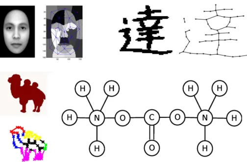
Nowadays, the application of graph-based representation techniques to pattern recog-nition and machine learning is becoming more and more popular. When we need to classify objects with complex internal structures, it is not always possible to construct feature vectors that capture important discriminative information between object classes. These difficulties lead to the use of more complex techniques, in particular, graph-based representation methods, where graphs are used to encode object features and structural relationships between them. Graphs provide a universal and flexible tool which may be used to describe objects in many application areas: computer vision, bioinformatics, chemoinformatics, etc.
The question of efficient graph-based representation is a problem in itself. De-pending on the area of application, different principles are used. In some cases, for example in chemoinformatics, it is very easy to construct a graph-based representa-tion of molecules. In other cases, for example in computer vision, this is more tricky,
14 LIST OF FIGURES
Figure 1: Examples of graph-based representations in computer vision and chemoin-formatics.
there are several ways to represent the same image: we can use segmentation graphs, shock graphs, contour graphs or their combination. Here, we do not consider how objects can be represented by graphs, we suppose that a particular graph-based rep-resentation method has already been chosen and we are interested in what happens afterwards.
Once a graph representation has been constructed, a central question arising in the context of pattern recognition is the question of graph (dis-)similarity measure. To be able to classify or cluster objects on the basis of their graph-based repre-sentations, we need to know how to compare graphs. A natural method for graph comparison is based on graph alignment with further evaluation of alignment qual-ity, the better the constructed alignment, the more similar the graphs. Construction of graph alignment is the subject of the graph matching problem where we seek a mapping between vertices of two graphs which optimally aligns the graph struc-tures. The graph matching problem is among the most important challenges of graph processing, and plays a central role in various fields of pattern recognition. Usu-ally, the optimality refers to the alignment of graph structures and, when available,
1. THE GRAPH MATCHING PROBLEM 15 of vertex labels, although other criteria are also possible. A non-exhaustive list of graph matching applications includes document processing tasks like optical charac-ter recognition [Lee and Liu, 1999; Filatov et al., 1995], image analysis (2D and 3D) [Wang and Hancock, 2006; Luo and Hancock, 2000; Carcassoni and Hancock, 2003; Schellewald and Schnorr, 2005], and bioinformatics [Singh et al., 2008; Wang et al., 2004; Taylor, 2002]. Figure 1 gives some examples where graph matching can be used to compare graph-based representations of different objects such as images and molecules.
We formulate the graph matching problem as a least square optimization problem on the set of permutation matrices
F (P ) = ||AG− P AHPT||2F
P ∈ P, (1)
where AGdenotes the adjacency matrix of graph G, AH denotes the adjacency matrix
of graph H, and P denotes a permutation matrix. Here, for simplicity, we suppose that the graphs have the same number of vertices, the general case of graphs of different sizes is considered in Section 1.3.3. Adjacency matrices are square binary (or real-valued) matrices. The set of permutation matrices P is defined as a set of square binary matrices with only one non-zero element in each row and each column P = {P ∈ {0, 1}N × N : P 1
N = 1N, PT1N = 1N}. We use permutation matrices
to encode matchings between graphs, Pij equals one if vertex i of graph G is aligned
with vertex j of graph H. Function F (P ) in (1) represents the discrepancy between the graphs after matching P . If graphs G and H are simple unweighted graphs (with binary adjacency matrices), then F (P ) corresponds to the number of edges which are present in one graph but not in the other. In the case of weighted graphs, F (P ) represents the total difference between all overlapping edges.
Problem (1) is a difficult combinatorial problem (NP-hard in the general case). While some methods based on incomplete enumeration may be applied to search for an exact optimal solution in the case of small or sparse graphs, only approximate algorithms that usually find non-optimal solutions but are more scalable can be used
16 LIST OF FIGURES for large non-sparse graph matching. Many such approximate algorithms have been proposed, see e.g., the review by Conte et al. [2004]. Roughly speaking, there are three main categories of approximate algorithms.
The first group consists of approximate tree search algorithms [Bunke, 1983]. The general idea of these algorithms is quite simple, we construct the global mapping iteratively. First, we match the first vertex of graph G to a vertex of graph H, then at each step we match a new pair of vertices in order to maximize the current number of overlapping edges.
The second category represents spectral methods [Umeyama, 1988; Caelli and Kosinov, 2004; Leordeanu and Hebert, 2005; Cour et al., 2006; Leordeanu et al., 2007]. For ex-ample, Umeyama [1988]; Caelli and Kosinov [2004] use the spectral decomposition of graph adjacency matrices
AG = VGΛGVGT, AH = VHΛHVHT.
Rows of VGand VH can be seen as spectral coordinates of graph vertices, therefore
to construct a matching between G and H, we match vertices with similar spectral coordinates.
The third category includes methods based on a relaxation of the optimization problem (1) [Almohamad and Duffuaa, 1993; Gold and Rangarajan, 1996].
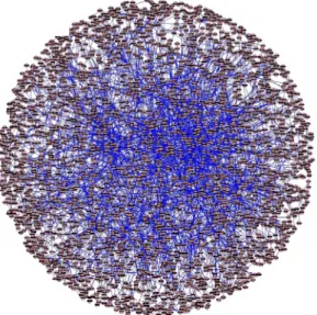
Defining a similarity measure for graphs is not the only application where graph matching algorithms may be of great use. In classification or clustering problems we use graph matching as a similarity measure between objects of interest i.e the value of function F (P ), but we never use the optimal mapping itself. In some bioin-formatics applications, the situation is quite the opposite, we are interested in the matrix P rather than in F (P ). An important example of such an application is the alignment of biological networks. For example, when we consider proteprotein in-teraction networks (see Figure 2), our objective is to find a mapping between proteins of two species which maximizes the number of conserved interactions. This problem is an instance of the graph matching problem where proteins correspond to graph
1. THE GRAPH MATCHING PROBLEM 17
Figure 2: Fly protein-protein interaction network. Vertices (nodes) represent proteins and edges correspond to protein-protein interactions.
vertices, and protein-protein interactions correspond to graph edges. Once an align-ment between protein-protein interaction networks is constructed, the matched pairs of proteins can be seen as “equivalent” proteins playing similar functional roles.
An important drawback of the existing formulation (1) is that it is based on a one-to-one correspondence between graphs. In many applications, it seems more nat-ural to consider many-to-many mappings. For example, in computer vision, in some situations the same object may have different graph-based representations depending on noise, point of view and other factors. In such a case, we may need to match several vertices to one vertex, or groups of vertices to groups of vertices.
1.1
Contribution & Perspectives
In the present work, we propose a new graph matching algorithm based on convex-concave programming. The convex-convex-concave programming formulation is obtained by rewriting the weighted graph matching problem as a least square problem on the set of permutation matrices and relaxing it to two different optimization problems: a quadratic convex and a quadratic concave optimization problem on the set of doubly
18 LIST OF FIGURES stochastic matrices. The concave relaxation has the same global minimum as the initial graph matching problem, but the search for its global minimum is still a hard combinatorial problem. We therefore construct an approximation of the concave problem solution by following a solution path of a convex-concave problem obtained by linear interpolation of the convex and concave formulations, starting from the convex relaxation. This method allows to easily integrate the information on graph label similarities into the optimization problem, and therefore to perform labeled weighted graph matching. A detailed description of this method is presented in Chapter 2.
The alignment of protein-protein interaction networks is the subject of several research papers. Bandyopadhyay et al. [2006] proposed to use a Markov random fields model, and Singh et al. [2008] introduced the IsoRank method inspired by the PageRank algorithm. In Chapter 3 we reformulate PPI alignment as a graph match-ing problem, and investigate how state-of-the-art graph matchmatch-ing algorithms can be used for that purpose. We differentiate between two alignment problems, depending on whether strict constraints on protein matches are given, based on sequence simi-larity, or whether the goal is instead to find an optimal compromise between sequence similarity and interaction conservation during alignment. We propose new methods for both cases, and assess their performance on the alignment of the yeast and fly PPI networks. The new methods consistently outperform state-of-the-art algorithms, retrieving in particular 78% more conserved interactions than IsoRank for a given level of sequence similarity.
To deal with the many-to-many graph matching problem, we can use several alternative approaches. Tree search algorithms can be easily generalized to the case of many-to-many matching. In the many-to-many case, the size of the optimization set is much larger, so when we match a new pair of vertices, one of them may be already matched to another vertex. Nevertheless, the core of the tree search algorithm for many-to-many matching is the same as in the one-to-one case. Spectral methods also have a natural generalization to the many-to-many case. Now, instead of matching pairs of vertices having similar spectral coordinates, we cluster all vertices on the basis of their spectral representations, then vertices from the same cluster are matched to
1. THE GRAPH MATCHING PROBLEM 19 each other.
In Chapter 4 we show how the many-to-many graph matching problem can be reformulated as a least square optimization problem. To the best of our knowledge, this is the first attempt to give a compact formulation of the many-to-many graph matching problem and one of the advantages of this formulation is that it leads to a natural approximate algorithm based on a continuous relaxation. The new algorithm works significantly better than existing approaches based on tree search and spectral decomposition.
Concerning future perspectives, there are a lot of interesting things to be done. The PATH algorithm probably can be further improved by construction of tighter convex and concave relaxations. The current procedure for processing directed graphs is based on a transformation of directed graph matching to undirected graph matching by doubling the number of vertices, but it would be better to run the PATH algorithm directly on directed graphs.
Since graph matching methods show good performance in the alignment of protein-protein interaction networks, it would be worth testing them on other types of bio-logical networks such as gene co-expression networks. Another interesting direction is the so called multi-matching problem where we seek a simultaneous alignment of several networks. In this case, the problem is formulated as follows. We have three or more graphs, for instance, G, H and B and our objective is to find an alignment of the graphs which minimize the total discrepancy between all triples of overlapping edges (gij, hij and bij)
discrepancy = (gij − hij)2+ (gij− bij)2+ (bij− hij)2.
Finally, we can formulate the three-graph multi-matching problem in the following way min PH,PB||G − P HHPHT||2F + ||G − PBHPBT||F2 + ||PBHPBT − PHHPHT||2F subject to PB, PH ∈ P (2)
20 LIST OF FIGURES or in the general case with n graphs G1,. . . ,Gn
min P1,P2,...,Pn X i,j ||PiGiPiT − PjGjPjT||2F subject to P1 = I, P2, . . . , Pn∈ P. (3) The majority of graph matching algorithms can be generalized to the multi-matching case, and it seems that this generalization may be quite useful is such fields of application as bioinformatics (synchronized alignment of biological networks corre-sponding to several species like Human-Mouse-Fly) or computer vision (synchronized alignment of graphs representing the same object).
2
Phrase-based statistical machine translation
One of the most famous challenges in natural language processing (NLP) is how to teach computers to translate texts. The objective is to construct a computer algo-rithm which can translate sentences from a source language (for example, French) to a target language (for example, English). There are two major groups of meth-ods for machine translation: rule-based systems and statistical machine translation (SMT) methods. Rule-based systems use linguistic rules defined by a human expert. SMT methods learn a translation model by themselves from a parallel bilingual text corpora (set of sentences in the source language and their translations in the target language). Also, there exist so called hybrid translation models where one tries to combine the best features of rule-based systems with the best of SMT models.
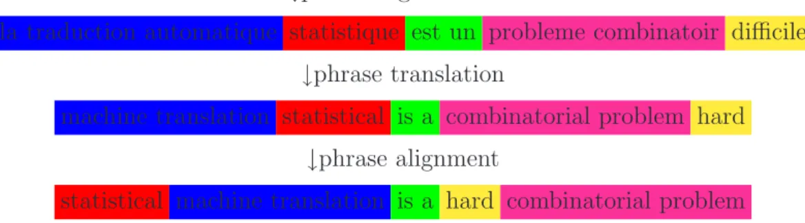
Ones of the most successful SMT systems are so-called Phrase-Based SMT mod-els. They use aligned sequences of words, called biphrases, as building blocks for translations. Figure 3 presents an illustration of PB-SMT. Roughly speaking, first, we segment the source sentence into blocks, then we translate them and finally the translated blocks are aligned in order to construct a correct sentence according to the target language. Note that in practice, “segmentation”, “phrase translation” and “alignment” are performed simultaneously and not step by step.
2. PHRASE-BASED STATISTICAL MACHINE TRANSLATION 21 la traduction automatique statistique est un probl`eme combinatoire difficile
↓phrase segmentation
la traduction automatique statistique est un probleme combinatoir difficile ↓phrase translation
machine translation statistical is a combinatorial problem hard ↓phrase alignment
statistical machine translation is a hard combinatorial problem
Figure 3: An example of phrase-based statistical machine translation process. Source and target parts of the same biphrases are highlighted by the same color.
problem) are called biphrases, so the translation process can be seen as a procedure
where, first, we cover the source sentence by a set of biphrases and then we permute the selected biphrases in order to construct a plausible translation.
The entire translation, consisting of selected biphrases and a biphrase permutation is usually called alignment a. PB-SMT models score alternative candidate translations for the same source sentence based on a log-linear model of the conditional probability of translation given the source sentence
p(T, a|S) = 1 ZS
expX
k
λkhk(S, a, T ) , (4)
where the hk’s are features, that is, functions of the source string S, of the target
string T , and of the alignment a (a already contains T but to emphasize that our objective is to construct T , we write (T, a) instead of just a). The λk’s are weights and
ZS is a normalization factor that guarantees that p is a proper conditional probability
distribution over the pairs (T, a). During the training phase, we estimate all model parameters λ and construct a dictionary of biphrases, then to translate a new sentence S (inference phase) we have to solve the following optimization problem
(T∗, a∗) = arg max
22 LIST OF FIGURES Problem (5) is called the Decoding problem.
The majority of PB-SMT models use the following list of features (siand tidenote
the source and target components of biphrases)
Local features Non-local features
Forward probabilities p(eti|esi) Language model p(eti|eti−1, . . . , eti−n)
Reverse probabilities p(esi|eti) Distortion |pos(esi) − pos(esi−1)|
Phrase lengths length(eti)
Local features depend only on individual biphrases, this means that they influence only the choice of biphrases, not their permutation. Non-local features depend on consecutive biphrases, they control both the permutation and choice of biphrases. If we use only local features in our translation model, then the decoding problem can be solved exactly in polynomial time, otherwise if we use non-local features such as the language model, then the decoding problem becomes NP-hard.
2.1
Contribution & Perspectives
Since, in the general case, the decoding problem is too hard to be solved exactly, approximate methods are normally used. The most used strategy for the decoding problem is the so-called beam-search algorithm which is a variant of the tree search strategy. In our joint work with Marc Dymetman and Nicola Cancedda from Xerox Research Center Europe (XRCE) we proposed an alternative decoding algorithm. We showed that the decoding problem is equivalent to the traveling salesman problem (TSP), a well known problem in operational research.
Given a non-directed graph G on N vertices, where the edges carry real-valued costs, the TSP problem consists in finding a tour of minimal total cost, where a tour (also called Hamiltonian Circuit) is a “circular” sequence of vertices visiting each vertex of the graph exactly once.
In Chapter 5, we propose a procedure which transforms any decoding problem into a traveling salesman problem. Given a new sentence S, this procedure constructs a graph where the optimal TSP tour corresponds to the solution of the decoding prob-lem. Besides the general interest in this transformation for understanding decoding,
3. COMPARISON OF PROTEIN BINDING POCKETS 23 it also opens the door to the direct application of a variety of existing TSP algorithms to SMT. Our experiments on synthetic and real data show that fast TSP algorithms can handle selection and reordering in SMT comparably or better than the state-of-the-art beam-search strategy, converging on solutions a higher objective function in a shorter time.
For the moment, we use classical TSP algorithms, and one of the interesting future directions is to further improve the optimization strategy by taking into account the special structure of the decoding graph.
3
Comparison of protein binding pockets
One of the main goals of structural biology is to predict, from the 3D fold of a protein, its interacting partners, which in turn is related to its molecular function. Understanding this structure-function relationship is still an open question, and no reliable tool is available to make such a prediction. Current efforts concentrate on local 3D approaches, focusing on identification and comparison of binding pockets, in order to predict the natural ligand for a protein, with the underlying idea that proteins sharing similar binding sites are expected to bind similar ligands. The same strategy also applies to the problem of identifying new drug precursors for a therapeutic target protein.
Binding pockets may be seen as 3D cavities on the protein surface (see Figure 4), we are interested in a method which will be able to detect pockets binding the same ligand on the basis of their 3D structure. Given such a method, we will be able to predict binding ligands for new, previously, unseen proteins.
3.1
Contribution & Perspectives
In Chapter 6, we propose an approach in which binding pockets are represented by clouds of atoms in 3D space potentially baring additional labels such as partial charge or atom type. The new similarity measure is based on the alignment of protein pockets with the further use of a convolution kernel between 3D point clouds.
24 LIST OF FIGURES
Figure 4: An illustration of an ATP binding pocket with the ATP ligand inside. Let P = (xi, li)Ni=1 denote a binding pocket consisting of N atoms, where xi ∈ R3
is a 3D vector representing atom coordinates, and liis a label (discrete or real valued)
that may be used to bare additional information on the atoms (for example, atom type, atom partial charge, or amino acid type).
A classical approach for pocket comparison consists in iterative pocket align-ment and further counting of overlapping atoms, usually within a tolerance of 1˚A [Willett et al., 1986]. The alignment is made to maximize the number of overlapping atoms, which is generally a good indicator of pocket similarity.
However, atoms may have different positions but play equivalent roles in ligand binding, and the role of one atom in one pocket may be played by a group of atoms in another pocket. These observations lead us to the idea of an alternative smooth score which does not count the number of overlapping atoms, but rather uses a weighted number of atoms having closed positions. Given two pockets P1 and P2 the similarity
measure K(P1, P2) is defined as follows
K(P1, P2) = X xi∈P1 X yj∈P2 e−||xi−yj || 2 2σ2 . (6)
4. PUBLICATIONS 25 This similarity measure represents a positive definite kernel, σ characterizes the sen-sitivity of the similarity measure (6) to the relative displacements of atoms.
In practice, formula (6) is not fully appropriate, because the proposed measure is not invariant under rotations and translations of the binding pockets. Therefore, we define a similarity measure sup-CK as the maximum of (6) over all possible rotations and translations of one of the two pockets:
sup-CK(P1, P2) = max R,yt X xi∈P1,yj∈P2 e||xi−(Ryj +yt)|| 2 2σ2 , (7)
This approach has shown good performance on several benchmark datasets in com-parison with such methods as the Tanimoto index [Willett et al., 1986], the SitesBase algorithm [Gold and Jackson, 2006], the MultiBind algorithm [Shulman-Peleg et al., 2008] and a method based on real spherical harmonic expansion coefficients [Morris et al., 2005].
Regarding future research directions, it would be interesting to couple the pro-posed similarity measure with some similarity measure between ligands in order to further improve the prediction performance. Then such a combination may be a good basis for the development of a public web server for protein-ligand interaction prediction.
4
Publications
The results presented in this thesis were published in the following papers.
Chapter 2: M. Zaslavskiy, F. Bach, J-P. Vert A Path Following Algorithm
for the Graph Matching Problem, “IEEE Transactions on Pattern Analysis and Machine Intelligence”, Dec. 2009.
Chapter 3: M. Zaslavskiy, F. Bach, J-P. Vert Global alignment of
pro-tein–protein interaction networks by graph matching methods “Bioin-formatics Oxford” (presented at ISMB-ECCB 2009).
26 LIST OF FIGURES
Chapter 5: M. Zaslavskiy, M. Dymetman, N. Cancedda Phrase-Based
Sta-tistical Machine Translation as a Traveling Salesman Problem “Pro-ceedings of the 47th Annual Meeting of the Association for Computational Linguistics (ACL-IJCNLP 2009)”, Jul. 2009.
Chapter 6: B. Hoffmann, M. Zaslavskiy , J-P. Vert, V. Stoven A new protein
binding pocket similarity measure based on comparison of 3D atom clouds: application to ligand prediction, conditionally accepted to BMC Bioinformatics, 2009
Part I
Graph matching
Chapter 1
Introduction and history of the
graph matching problem
The goal of this chapter is to introduce the graph matching problem. We compare alternative formulations of graph matching and trace the evolution of ideas related to graph comparison.
1.1
Basic definitions and notations
A graph G = (V, E) of size N is defined by a finite set of vertices V =
{1, . . . , N} and a set of edges E ⊂ V × V . Each graph can be represented by a square adjacency matrix A of size |V | × |V |, where Aij is equal to one
if there is an edge between vertex i and vertex j, and zero otherwise.
In weighted graphs, edges have associated labels(weights). Weights are
usu-ally real numbers. Unweighted graphs are described by binary adjacency ma-trices.
G is called an undirected graph if and only if A
G
ij = AGji.
G
′ = (V′, E′) is a subgraph of graph G, if V′ ⊂ V and E′ ⊆ V′ × V′∩ E. G′
is called an induced subgraph of G if E′ = V′× V′ ∩ E. G′.
1.2. FORMULATION OF THE GRAPH MATCHING PROBLEM 29
A matching or an alignment of two graphs is a mapping between the vertices
of two graphs
f : VG→ VH.
If graphs have the same number of vertices N and f is a bijection, then such a matching is called one-to-one. A one-to-one matching can be encoded by a permutation matrix. The set of permutation matrices is defined as follows
P = {P ∈ {0, 1}N ×N : P 1N = 1N, PT1N = 1N}, (1.1)
where 1N is a column vector with N ones.
Two graph G and H are called isomorphic if and only if there exists a
one-to-one mapping f : G → H such that (i, j) ∈ EG↔ (f(i), f(j)) ∈ EH
1.2
Formulation of the graph matching problem
The first formulation of the graph matching problem was proposed by Tsai and Fu [1979]. Graph matching was introduced as a noisy version of the graph isomorphism problem. Such a definition is quite natural for understanding the graph matching problem. Checking for graph isomorphism, we can only verify whether two graphs are the same or not, but in many applications, this is not enough. Sometimes even if graphs are different, we need to know how different they are, in other words, instead of a binary Yes/No answer for the graph isomorphism problem, we need a graph (dis-)similarity measure with more gradations. A possible solution is to use the size of the maximum common subgraph (MCS) as a measure of graph similarity, or its normalized version
Sim(G, H) = |MCS(G, H)|
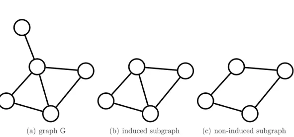
max(|G|, |H|), (1.2) where |G| denotes the number of edges in G. The classical definition of the maximum common subgraph is based on the notion of induced subgraphs. Figure 1.1 illustrates the difference between induced and simple subgraphs. Subgraph G′ of graph G is
30 CHAPTER 1. INTRODUCTION
(a) graph G (b) induced subgraph (c) non-induced subgraph
Figure 1.1: Examples of induced and non-induced subgraphs. connecting these vertices.
Usually, the maximum common subgraph is defined as the maximum induced common subgraph, but in our case, to measure similarity (1.2) between graphs, we can use both versions: induced and non-induced.
However, this approach is appropriate only in the case of simple unweighted graphs. If graph edges have associated weights (which is often the case in real appli-cations) then it becomes difficult to use the notion of maximum common subgraph. For instance, it is unreasonable to seek a common subgraph with exactly the same edge weights if these weights are real numbers. Of course, one can always discretize weights and follow the MCS approach, but this may lead to information loss.
To understand what would be a better alternative to the discretization schema, let us look at the maximum common subgraph problem from a different point of view. Let us suppose, that we do not consider only induced subgraphs, but all kinds of subgraphs. And let us suppose, for simplicity, that graphs G and H have the same number of vertices N . Then the extraction of the MCS may be seen as a procedure where we seek an alignment of two graphs which provides the maximum number of overlapping edges. This idea is illustrated in Figure 1.2.
The optimal alignment may be defined as an alignment maximizing the number of overlapping edges (solid lines) or minimizing the number of non-overlapping edges (dotted lines). Alignment of two graphs may be encoded by the permutation matrix
1.2. FORMULATION OF THE GRAPH MATCHING PROBLEM 31
(a) graph G (b) MCS(G,H) (c) graph H
Figure 1.2: The maximum common subgraph (solid edges) as a result of graph align-ment.
P where Pij = 1 if vertex i of graph G is matched to vertex j of graph H and zero
otherwise. Let G and H also denote the adjacency matrices of corresponding graphs, then the number of non-overlapping edges under matching P can be expressed as follows
F (P ) = 1
2||G − P HP
T
||2F (1.3)
where || ||F denotes the Frobenius norm ||A||2F =
P A2
ij. Function F (P ) expresses the
number of non-overlapping edges, and therefore the problem of MCS identification may be rewritten as the following optimization problem
min
P F (P )
subject to
P ∈ {0, 1}N ×N, P 1N = 1N, PT1N = 1N
(1.4) The choice of the Frobenius norm is quite arbitrary, it can be replaced by any matrix norm, for instance, lp (1 ≤ p ≤ ∞). The optimization set in (1.4) is exactly the set of
permutation matrices. Now, given (1.3,1.4), the generalization to the case of weighted graphs is straightforward. The introduction of edge weights corresponds to replacing binary elements of matrices G and H by real numbers. Optimization problem (1.4) in the case of weighted graphs means that we seek a matching which minimize the
32 CHAPTER 1. INTRODUCTION total difference between all aligned edges. Note, that if we consider weighted graphs, there is no longer any difference between induced and non-induced subgraphs, the absence of an edge between two vertices may be considered to be an edge with zero weight.
The formulation of graph matching in the form of (1.4) was given in [Umeyama, 1988], where Umeyama rewrote the idea of inexact graph isomorphism [Tsai and Fu, 1979] in the form of an optimization problem. We use this formulation, however there exist alternative formulations of the graph matching problem such as the graph edit distance. In the next section, we briefly discuss the relation between formulation (1.4) and other existing definitions of the graph matching problem.
1.3
Alternative formulations of the graph
match-ing problem
In the general case, the graph matching problem is formulated as follows. Given two graphs, find the correspondence between their vertices which provides the best alignment of graph structures. This definition is informal since the notion of best alignment is not uniquely defined. Depending on how we define it, we get different formulations of the graph matching problem.
1. Exact Matching
Graph isomorphism: check whether two graphs are the same.
Subgraph isomorphism: check whether the smallest graph is a subgraph of
the biggest one. 2. Inexact Matching
MCS: the maximum common subgraph problem. Least square formulation: minimize (1.4).
1.3. ALTERNATIVE FORMULATIONS OF GRAPH MATCHING 33 The variants of exact matching may be seen as particular cases of the least square formulation. If graphs G and H are of the same size, then they are isomorphic if and only if minPF (P ) = 0. Similarly, if G is smaller than H, then G is a subgraph of H
if and only if minP F (P ) = |H| − |G|.
In the case of inexact matching, along with the least square formulation, another popular approach is based on the graph edit distance. The graph edit distance was proposed by Tsai and Fu [1979]; Bunke [1983]. It was defined as the minimum amount of distortion that we need to transform one graph into another. Graph transformation is performed via insertions, deletions and substitutions of graph vertices and edges. Each operation has an associated cost, and the transformation distortion is defined as the total cost of all operations employed. Interestingly, in many cases, the graph edit distance may be rewritten in terms of the least square formulation, we will show how this can be done in Section 1.3.5, but first we consider how the least square formulation may be further generalized to include information on vertex labels, how the graph matching problem may be rewritten in the form of a quadratic assignment problem and what can be done if graphs have a different number of vertices.
1.3.1
Vertex labels
An interesting instance of the graph matching problem is the matching of labeled graphs. In that case, graph vertices have associated labels, which may be numbers, categorical variables, etc... The important point is that there is also a similarity mea-sure between these labels. Therefore, when we search for the optimal correspondence between vertices, we search a correspondence which matches not only the structures of the graphs but also vertices with similar labels. Some widely used approaches for this case only use the information about similarities between graph labels. In vision, one such algorithm is the shape context algorithm proposed by Belongie et al. [2002], which involves an efficient algorithm of node label construction. Another example is the BLAST-based algorithms in bioinformatics such as the Inparanoid algorithm [Brein et al., 2005], where correspondence between different protein networks is estab-lished on the basis of BLAST scores between pairs of proteins. The main advantages
34 CHAPTER 1. INTRODUCTION of all these methods are their speed and simplicity. However, these methods do not take into account information about the graph structure. Some graph matching meth-ods try to combine information on graph structures and vertex similarities, examples of such method are presented in [Schellewald et al., 2001; Singh et al., 2008].
The least square formulation may be easily adjusted to include information on the vertex labels. Let gi and hj denote vertex labels in graphs G and H
correspond-ingly. The optimal alignment of two graphs should not only match edges with similar weights, but also put into correspondence vertices having similar labels. The new objective function is the following modification of (1.3)
Fα(P ) = (1 − α)||G − P HPT||2F + αtrCPT , (1.5)
where C ∈ RN ×N encodes pairwise dissimilarities between vertex labels of two graphs
Cij = dissim(gi, hj), and α controls the trade-off between edge and vertex alignment
components, the greater parameter α, the more attention we pay to alignment of vertices with similar labels.
1.3.2
Quadratic assignment problem
An interesting fact about the least square formulation is that it can be seen as an instance of the quadratic assignment problem. The quadratic assignment problem is formulated as follows max P trAP TBP subject to P ∈ {0, 1}N ×N, P 1N = 1N, PT1N = 1N, (1.6) where A and B are N × N real valued matrices.
The transformation of (1.4) to (1.6) is quite simple, the optimization set is exactly the same ( the set of permutation matrices) and we only need to rewrite the objective
1.3. ALTERNATIVE FORMULATIONS OF GRAPH MATCHING 35 function
||G − P HPT||2F = ||GP − P HP ||2F
=trPTGTGP − 2trPTGTP H + trHTPTP H = trGTG − 2trGTP HPT + trHTH now since trGTG and trHTH do not depend on P
min
P ||G − P HP T
||2F ⇔ maxP trGTP HPT.
The information on vertex pairwise similarities (see the previous section) may be also included in the QAP formulation, it corresponds to adding a linear term to the QAP objective function. This extended formulation of QAP is usually called the generalized quadratic assignment problem.
1.3.3
Matching graphs of different sizes
Often in practice we have to match graphs of different sizes NG and NH (NG< NH).
In this case we have to match all vertices of graph G to a subset of vertices of graph H. In the usual case when NG = NH, the error (1.3) corresponds to the number of
mismatched edges (edges which exist in one graph and do not exist in the other one). When we match graphs of different sizes the situation is a bit more complicated. Let VH+ ⊂ VH denote the set of vertices of graph H that are selected for matching to
vertices of graph G, let VH− = VH \ VH+ denote all the rest. Therefore all edges of
the graph H are divided into four parts EH = EH++∪ EH+−∪ EH−+∪ EH−−, where EH++
are edges between vertices from VH+, EH−− are edges between vertices from VH−, EH+− and EH+− are edges from VH+ to VH− and from VH− to VH+ respectively. For undirected graphs the sets EH+− and EH+− are the same (but, for directed graphs they would be different). The edges from EH−−, EH+− and EH−+ are always mismatched and a question is whether we have to take them into account in the objective function or not. According to the answer we have three types of matching error (four for directed graphs) with interesting interpretations.
36 CHAPTER 1. INTRODUCTION 1. We count only the number of mismatched edges between G and the chosen subgraph H+⊂ H. It corresponds to the case when the matrix P from (1.3) is
a matrix of size NG× NH and NH − NG columns of P contain only zeros.
2. We count the number of mismatched edges between G and the chosen subgraph H+ ⊂ H. And we also count all edges from E−−
H , E
+−
H and E −+
H . In this case
P from (2.1) is a matrix of size NH× NH. And we transform AG into a matrix
of size NH × NH by adding NH − NG zero rows and zero columns. It means
that we add dummy isolated vertices to the smallest graph, and then we match graphs of the same size.
3. We count the number of mismatched edges between G and chosen subgraph H+ ⊂ H. And we also count all edges from E+−
H (or E −+
H ). It means that
we count matching error between G and H+ and we count also the number of
edges which connect H+ and H−. In other words we are looking for subgraph
H+ which is similar to G and which is maximally isolated in the graph H.
Figure 1.3.3 illustrates different types of matching error described above.
Each type of error may be useful according to the context and interpretation, but a priori, it seems that the best choice is the second one where we add dummy nodes to the smallest graph. The main reason is the following. Suppose that graph G is quite sparse, and suppose that graph H has two candidate subgraphs H+
s (also quite
sparse) and Hd+ (dense). The upper bound for the matching error between G and H+
s is #VG + #VHs+, the lower bound for the matching error between G and H
+ d is
#VH+
d − #VG. So if #VG + #VH +
s < #VHd+ − #VG then we will always choose the
graph H+
s with the first strategy, even if it is not similar at all to the graph G. The
main explanation of this effect lies in the fact that the algorithm tries to minimize the number of mismatched edges, and not to maximize the number of well matched edges. In contrast, when we use dummy nodes, we do not have this problem because if we take a very sparse subgraph H+ it increases the number of edges in H−(the
common number of edges in H+ and H− is constant and is equal to the number of
1.3. ALTERNATIVE FORMULATIONS OF GRAPH MATCHING 37
Figure 1.3: Matching of graphs with different number of vertices. On the left graph G is drawn in red, edge set EH++ is drawn in black (matched edges) and green (mis-matched edges), EH+− in blue and EH−− in brown. On the right, the same edge sets are represented in terms of the adjacency matrices: green area corresponds to EH++, blue area to EH+− and brown area to EH−−
1.3.4
l
1and other alternatives to the l
2norm in the graph
matching problem
To solve the graph matching problem, we seek a mapping between the vertices of two graphs which minimizes the difference between the adjacency matrix of one graph and the permuted adjacency matrix of the second graph. In the least square formulation, the difference is measured by the l2 norm, but, of course, any other matrix norm may
be used. For example, the LP based approach [Almohamad and Duffuaa, 1993] uses the l1 norm, other choices like lp norms with different p are possible as well. Note,
if we consider only unweighted graphs (with binary adjacency matrices), then all lp
norms (power p) are equivalent
38 CHAPTER 1. INTRODUCTION
1.3.5
Graph edit distance
The graph edit distance, which has already been defined above, is based on the no-tion of an optimal transformano-tion of one graph into another. The graph edit distance may be seen as a generalization of the string edit distance. In the case of strings, the set of editing operations consists of deletion, insertion and substitution of char-acters, and in the case of graphs, we consider deletion, insertion and substitution of vertices and edges. Below we cite the definition of the graph edit distance used in [Neuhaus and Bunke, 2007]
Definition 1 Given two graphs G and H, the graph edit distance between G and H
is defined by ged(G, H) = min (e1,...,ek)∈P (G,H) k X 1 c(ei) , (1.7)
where P (G, H) defines the set of all possible transformations G → H, and c(e1)
denotes the costs of editing operations: deletion, insertion and substitution of graph vertices and edges.
Each edit operation has an associated cost. Usually, these costs are defined as func-tions of edge and vertex labels. A natural hypothesis about edit operafunc-tions is that a simple operation is always preferable to a sequence. For instance, substitution of vertex g by vertex h may be done via “substitution” or via “deletion+insertion”, and a reasonable assumption is that the “substitution” cost should be smaller than the total “deletion+insertion” cost. Under this hypothesis, the notion of optimal edit path loses the idea of an ordered set of edit operations, all edit transformations may be applied simultaneously. Now it becomes clear how the graph edit distance may be related to formulation (1.5). Substitution of vertex g by vertex h means that these two vertices are matched to each other, the same is true for edges. When we insert a new vertex(edge) in graph G and match it to an existing vertex (edge) in graph H, it is somehow equivalent to deletion of vertices (edges) in graph H. Finally, the graph edit distance transformation may be seen as a matching of vertices (edges) which are chosen to be substituted, and then deletion of all unmatched elements in both graphs. Deletions in both graphs may be seen as matching of deleted vertices
1.3. ALTERNATIVE FORMULATIONS OF GRAPH MATCHING 39
Figure 1.4: The graph edit path as simultaneous matching of all graph vertices and edges. Substitution operations correspond to matching of vertices and edges, vertex deletions correspond to alignment with dummy vertices (blue), edge deletion corre-sponds to alignment with nothing.
to dummy vertices. Figure 1.3.5 gives an illustration of this schema.
To finish the reformulation we have to clarify what happens with insertion, deletion and substitution costs when we reformulate (1.7) as (1.5). Usually, edit operation costs are defined as functions of vertex and edge labels. Vertex operation costs may be encoded directly in the matrix C (see (1.5)), the situation with edges is a bit more complicated. If edge labels are real valued weights, and substitution and deletion costs are defined as
subst(gi, hj) = (gi− hj)2, del(gi) = gi2, del(hi) = h2i ,
then the objective function defined in (1.5) equals the total cost of the edit path transformation. If, for instance, the costs of edit operations are defined as (see [Ambauen et al., 2003])
40 CHAPTER 1. INTRODUCTION then we have to replace the Frobenius norm in (1.5) by the l1 norm (see Section 1.3.4).
A similar adaptation of the objective function (1.5) should be made in the case of alternative edit operation costs.
1.3.6
Complexity of the graph matching problem
In some special cases, for example, when we restrict graph matching to graph isomor-phism, it is difficult to say what the complexity of the corresponding problem is. For the moment, there is no known polynomial algorithm for graph isomorphism, and at the same time we do not know whether this problem is NP-hard or not. However in the general case, the graph matching problem is NP-hard, this fact follows naturally from the equivalency of the quadratic assignment problem and graph matching of weighted directed graphs.
1.4
Early history of graph matching
In this section we try to trace the evolution of the ideas related to the problem of graph matching. This objective is rather ambiguous and vague, but we believe it may be interesting to trace back how people came to the idea of graph comparison.
The commonly accepted view is that the first paper related to graph theory was the paper on the Seven Bridges of K¨onigsberg written by Leonard Euler in 1735. At that time, the term “graph” had not been introduced, but the problem discussed in this paper is an example of a graph related problem. The term “graph” was introduced much later by James Sylvester in his article “Chemistry and algebra”, Nature, 1895. Interestingly, the roots of graph theory are closely related to what we see now as an application area for graph-based methods.
As mentioned in the previous section, the current formulation of the graph match-ing problem was given by Tsai and Fu [1979]. But from a more general point of view, the graph matching problem represents an approach to graph comparison, a problem which was known long before [Tsai and Fu, 1979]. In the previous section, we have shown that the graph isomorphism problem, the subgraph isomorphism problem and
1.4. EARLY HISTORY OF GRAPH MATCHING 41
Figure 1.5: An example of Crum Brown’s drawing: ammonic carbonate structure. the problem of the maximum common subgraph may be seen as particular cases of the graph matching problem. These problems are related to different aspects of graph comparison such as whether two graphs have the same structure, whether one graph is a subgraph of another and so on. The graph isomorphism problem seems to be the most studied variant of all graph comparison formulations. The number of pub-lications (sometimes containing wrong conclusions) on this topic is so big, that the graph isomorphism problem was called a graph isomorphism disease similarly to the four-colour problem [Read and Corneil, 1977].
It is hard to say when the graph isomorphism problem was formulated for the first time. By all appearances, the question about graph isomorphism arose at the same time that the term “graph” was introduced by J. Sylvester, and again it was closely related to existing problems in chemistry. In 1864 Alexander Crum Brown published a paper proposing a new system for the diagramic representation of molecules. His system is still popular and it corresponds exactly to how we draw graphs today (see Figure 1.5).
At this time several alternative representation systems were proposed by Couper, Loschmidt and Kekule, but the one by Crum Brown was the most successful. One of the reasons for this success is due to the fact that Crum Brown’s system provides an explanation of the phenomena of molecular isomerism. Isomers are chemical com-pounds having the same chemical composition but different physico-chemical proper-ties. For instance, Figure 1.6 shows two isomers: propan-1-ol and propan-2-ol known
42 CHAPTER 1. INTRODUCTION
(a) propylic alcohol (b) Friedel’s alcohol
Figure 1.6: Examples of chemical isomers: propan-1-ol and propan-2-ol at the time of Crum Brown as Friedel’s alcohol and propylic alcohol.
Obviously, the question of chemical isomerism is equivalent to the graph iso-morphism problem. Two substances with the same chemical composition represent different isomers if and only if their graphical notations correspond to non-isomorphic graphs.
The question of molecular isomers gave rise to graph enumeration theory. Roughly speaking, in the context of graph enumeration theory, we are interested in counting graphs with a particular property. The first works on this topic were done by Cayley [1874, 1859, 1875, 1877] where he proposed a method for counting different rooted trees with N vertices (Cayley used the term knot). So here, “different” means “non-isomorphic”, Cayley applied his method to count the number of isomers CnH2n+2.
Much later, P`oyla further developed this theory and proposed a basis for the general enumeration theory, a new branch in algebra.
About the same time that G.Poly`a worked on his enumeration theory, Hassler Withney published a paper called “Congruent graphs and connectivity of graphs”,
1932, where among other results he showed that two connected graphs are isomorphic
if and only if their line graphs are isomorphic 1. This paper is considered to be one
of the first papers establishing a theoretical fact about graph isomorphism. Withney did not propose an algorithm for the graph isomorphism problem, but nevertheless his result is quite important for us, since it provides a better understanding of graph
1
1.4. EARLY HISTORY OF GRAPH MATCHING 43 isomorphism, and actually addresses the graph isomorphism problem in the form as it is known today.
The next important steps in the development of graph isomorphism algorithms are related to the evolution of computing hardware. In 1954 Gotusso and Santolini wrote the article “A Fortran IV quasi-decision algorithm for the P-equivalence of two
matrices”. Two matrices G and H are P-equivalent if there exists a permutation
matrix P such that
G = P HPT.
While they did not consider the graph isomorphism problem directly, we know that the P-equivalence of graph adjacency matrices means that the corresponding graphs are isomorphic. Starting in the 1950s, a lot of papers were published proposing different algorithms for the graph isomorphism problem, we will not discuss them here, a good review of existing work on graph isomorphism was written by Read and Corneil [1977] and then completed by Gati [1979] and in a more recent technical report by Fortin [1996]. We would just like to mention two papers, one by Ray and Kirsch
“Finding Chemical Records by Digital Computers”, 1957 which is considered to be
one of the first papers in modern chemoinformatics, and another one by Sussenguth
“A graph theoretic algorithm for matching chemical structures”, 1963 where he further
developed the ideas of Ray and Kerisch and proposed to use (sub)-graph isomorphism methods for comparing chemical structures.
In the table below we cite key works which we believe had a significant impact on the understanding of the graph comparison problem. Further information on the historical development of graph theory and related concepts can be found in Biggs et al. [1976]; Diestel [2000]; Godsil and Royle [2000]; Bondy and Murty [1976].
Year Authors Paper & Comments
1735 L. Euler The first publication on a graph related problem: “Seven
Bridges of K¨onigsberg”.
1864 A. Crum Brum New graphic notation for chemical compounds (see Fig-ure 1.5), understanding the phenomena of chemical iso-merism.
44 CHAPTER 1. INTRODUCTION Year Authors Paper & Comments
1875 J. Sylvester His paper “Chemistry and Algebra” is about the similar-ity between the algebraic theory of binary quantics and the existing graphic representation of molecules. Intro-duction of the term graph.
1875 W. Clifford His work was mainly concentrated on the invariants of binary quantics (“Note on invariants of alternate
num-bers, used as a mean for determining the invariants and covariants of quantics in general”, “Binary forms of alternate variables”), W. Clifford proposed the
graph-based notation in this field.
1875-1877
A. Cayley “On the analytical forms called trees with application to the theory of chemical combinations”, 1875, “On the number of univalent radicals CnH2n−1”,1877. Cayley
was interested in how to count trees with a given num-ber of vertices (knots) and the potential application of such methods to the enumeration of molecular isomers 1927 J. Redfield His paper “The theory of group-reduced distributions”
was one of the first papers in graph enumeration theory. While this paper is not well known, it forestalls to some extent a lot of ideas from G. Poly`a’s paper on graph enumeration.
1929 A. Lunn and J. Senior
In their paper “Isomerism and Configurations”, they discuss how the theory of permutation groups may be used to enumerate molecular isomers.
1930-1935
G. Poly`a In his paper “A general combinatorial problem on groups
of permutations and the calculation of the number of isomers of organic compounds”, he builds the basis of
1.4. EARLY HISTORY OF GRAPH MATCHING 45 Year Authors Paper & Comments
1930-1932
H. Whitney Two papers of H. Whitney “Non-separable and planar
graphs”, 1930 and “Congruent graphs and the connectiv-ity of graphs”, 1932 address the problem of graph
iso-morphism as a pure mathematical problem and study different properties of isomorphic graphs.
1957 L. Ray, R. Kirsch
Their paper “Finding chemical records by digital
com-puters” is considered as one of the first papers in
chemoinformatics. They propose an information-retrieval process for the analysis of the dataset of known chemical compounds. While they paper is mainly con-ceptual, it includes some ideas about graph-based com-parison of molecules.
1957 L. Gatusso, A. Santolini
Formally speaking, their work “A Fortran IV quasi
de-cision algorithm for the P-equivalence of two matrices”
is not a graph theoretical paper, but since graph isomor-phism is equivalent to the P-equivalence of two matrices, this paper may be seen as one of the first papers provid-ing an algorithm for the graph isomorphism problem. 1963 E. Sussenguth E. Sussenguth further developed the ideas of L. Ray
and R. Kirsch. His paper “A graph theoretic algorithm
for matching chemical structures” is about how graph
isomorphism algorithms may be used to detect similar chemical compounds.