Universit´e de Montr´eal
Sequence to Sequence Learning and Its Speech Applications
par Ying Zhang
D´epartement d’informatique et de recherche op´erationnelle Facult´e des arts et des sciences
M´emoire pr´esent´e `a la Facult´e des arts et des sciences en vue de l’obtention du grade de Maˆıtre `es sciences (M.Sc.)
en informatique
April, 2018
Résumé
Les r´eseaux neuronaux r´ecurrents (RNN) ont ´et´e dominants dans le domaine de la parole au cours des derni`eres d´ecennies, ´etant donn´e leurs propri´et´es attrayantes de mod´elisation de s´equences. Les r´eseaux neuronaux convolutionnels (CNN) ont ´et´e pr´esent´es comme une alternative pour la mod´elisation de s´equences en raison de leur capacit´e `a r´eduire les variations spectrales et `a mod´eliser les corr´elations spectrales dans les caract´eristiques acoustiques pour la reconnaissance automatique de la parole (ASR). Des travaux r´ecents sugg`erent que les nombres complexes pour-raient ˆetre utilis´es comme une repr´esentation de caract´eristique plus riche que le spectre et qui pouvaient donc ˆetre b´en´efique pour les tˆaches li´ees `a la parole.
Dans la th`ese, nous abordons d’abord les concepts de base de l’apprentissage automatique, les blocs de construction de l’apprentissage profond et discutons des m´ethodes populaires capables de faire des mod´elisations s´equentielles, en particu-lier des r´eseaux de neurones convolutionnels, c´el`ebres en tant que r´eseaux feed-foward. Nous pr´esentons ensuite deux travaux de recherche li´es `a la mod´elisation s´equence-s´equence sur la parole. Premierement, nous introduisons une nouvelle ap-proche pour adresser la reconnaissance de la parole avec des r´eseaux de neurones convolutionnels qui montre des performances comparables avec leur homologue des r´eseaux neuronaux r´ecurrents. Deuxi`emement, nous pr´esentons un nouveau mo-d`ele, tirant parti de la repr´esentation dans le domaine complexe, et d´efinissons des circonvolutions complexes, des strat´egies complexes de normalisation par lots et d’initialisation de poids complexes. Le mod`ele a atteint l’´etat de l’art de la tˆache de pr´ediction du spectre de la parole dans un cadre r´ecurrent convolutionnel.
Mots cl´es: r´eseaux de neurones, apprentissage automatique, apprentissage profond, r´eseaux de neurones convolutionnels, mod´elisation de s´equences, recon-naissance de la parole, repr´esentation complexe
Summary
Recurrent Neural Networks (RNNs), which has the attractive properties of mod-elling sequences, has been dominant in speech field in the recent decades. Convo-lutional Neural Networks (CNNs) has been shown as an alternative to model se-quences because of its capacity of reducing spectral variations and modeling spectral correlations in acoustic features for automatic speech recognition (ASR). Recent work suggests that complex numbers could be used as a richer feature representa-tion than spectrum which may benefit the speech related tasks.
In the thesis, we first cover the basic concepts in machine learning, building blocks of deep learning and discuss the popular methods that are capable of doing sequence-to-sequence modelling, specially convolutional neural networks, which is famous as a class of feed-forward nets. We then present two research work re-lated to sequence-to-sequence modelling on speech. We introduce a new approach to address speech recognition with convolutional neural networks which shows the comparable results with their recurrent neural networks counterpart. In addition, we present a new model taking advantage of the representation in the complex domain and define complex convolutions, complex batch-normalization, complex weight initialization strategies. The new model results in state-of-the-art of speech spectrum prediction in a convolutional recurrent setting.
Keywords: neural networks, machine learning, deep learning, convolutional neural networks, sequence modelling, speech recognition, complex representation
Contents
R´esum´e . . . ii
Summary . . . iii
Contents . . . iv
List of Figures. . . vi
List of Tables . . . vii
List of Abbreviations . . . ix
Acknowledgments . . . x
1 Introduction to Deep Learning . . . 1
1.1 Machine Learning Basics . . . 1
1.1.1 Definition . . . 1
1.1.2 Tasks Categorization . . . 1
1.1.3 Empirical Risk . . . 2
1.1.4 Generalization . . . 3
1.2 Artificial Neural Networks . . . 4
1.2.1 Perceptron. . . 4
1.2.2 Multi-Layer Perceptrons . . . 5
1.2.3 Activation Function. . . 5
1.2.4 Cost Functions . . . 7
1.2.5 Optimization . . . 8
2 Sequence to Sequence Learning . . . 12
2.1 Concept . . . 12
2.2 Recurrent Neural Networks . . . 12
2.3 Long Short Term Memory . . . 14
2.4 Bidirectional Structure . . . 15
2.5 Convolutional Neural Networks . . . 15
2.5.1 Convolution . . . 16
2.5.3 Fully Connected Layer . . . 18
2.6 Sequence Loss Function . . . 18
2.6.1 Connectionist Temporal Classification. . . 18
3 Prologue to First Article . . . 21
4 Towards End-to-End Speech Recognition with Deep Convolu-tional Neural Networks . . . 22
4.1 Introduction . . . 22
4.2 Experiments . . . 25
4.2.1 Data . . . 25
4.2.2 Models . . . 25
4.2.3 Training and Evaluation . . . 25
4.2.4 Results. . . 26
4.3 Discussion . . . 26
5 Prologue to Second Article . . . 28
6 Deep Complex Networks . . . 29
6.1 Introduction . . . 29
6.2 Complex Building Blocks . . . 31
6.2.1 Representation of Complex Numbers . . . 31
6.2.2 Complex Convolution. . . 31
6.2.3 Complex Di↵erentiability . . . 32
6.2.4 Complex-Valued Activations . . . 33
6.2.5 Complex Batch Normalization . . . 34
6.2.6 Complex Weight Initialization . . . 36
6.2.7 Complex Convolutional Residual Network . . . 38
6.3 Experiments . . . 40
6.3.1 Image Recognition . . . 40
6.3.2 Automatic Music Transcription . . . 42
6.3.3 Speech Spectrum Prediction . . . 44
7 Conclusion . . . 46
List of Figures
1.1 The curve between training / generalization error and model capac-ity. X-axis denotes model capacity and Y-axis denotes the error. . . 3
1.2 A graphical illustration of perceptron algorithm . . . 4
1.3 A graphical illustration of multi-layer perceptron. . . 5
1.4 A graphical depiction of the di↵erence between BGD and SGD. SGD o↵ers noiser gradient in each iteration. . . 9
1.5 The detailed Adam algorithm showed in Kingma and Ba (2014) . . 10
2.1 A recurrent neural network unrolled in time (Figure adapted from Yoshua Bengio’s slides) . . . 13
2.2 The di↵erence between a bidirectional RNN and an unidirectional RNN. (Figure adapted from wikipedia) . . . 15
2.3 The convolution layer and max-pooling layer applied upon input fea-tures. . . 16
2.4 Diliated convolution on 2D data. Figure is adapted from Yu and Koltun (2015) . . . 17
4.1 Network structure for phoneme recognition on the TIMIT dataset. The model consists of 10 convolutional layers followed by 3 fully-connected layers on the top. All convolutional layers have the filter size of 3⇥ 5 and we use max-pooling with size of 3 ⇥ 1 only after the first convolutional layer. First and second numbers correspond to frequency and time axes respectively. . . 24
6.1 Complex convolution and residual network implementation details.. 32
List of Tables
4.1 Phoneme Error Rate (PER) on TIMIT. ’NP’ is the number of pa-rameters. ’BiLSTM-3L-250H’ denotes the model has 3 bidirectional LSTM layers with 250 units in each direction. In the CNN model, (3, 5) is the filter size. Results suggest that deeper architecture and larger filter sizes leads to better performance. The best performing model on Development set, has a test PER of 18.2 % . . . 27
6.1 Classification error on CIFAR-10, CIFAR-100 and SVHN⇤ using dif-ferent complex activations functions (zReLU, modReLU andCReLU). WS, DN and IB stand for the wide and shallow, deep and narrow and in-between models respectively. The prefixes R & C refer to the real and complex valued networks respectively. Performance di↵erences between the real network and the complex network using CReLU are reported between their respective best models. All models are constructed to have roughly 1.7M parameters except the modReLU models which have roughly 2.5M parameters. modReLU and zReLU were largely outperformed by CReLU in the reported experiments. Due to limited resources, we haven’t performed all possible experi-ments as the conducted ones are already conclusive. A ”-” is filled in front of an unperformed experiment. . . 38
6.2 Classification error on CIFAR-10, CIFAR-100 and SVHN⇤ using dif-ferent normalization strategies. NCBN, CBN and BN stand for a Naive variant of the complex normalization, complex batch-normalization and regular batch batch-normalization respectively. (R) & (C) refer to the use of the real- and complex-valued convolution respectively. The complex models use CReLU as activation. All models are constructed to have roughly 1.7M parameters. 5 out of 6 experiments using the naive variant of the complex batch normal-ization failed with the apparition of NaNs during training. As these experiments are already conclusive and due to limited resources, we haven’t conducted other experiments for the NCBN model. A ”-” is filled in front of an unperformed experiment. . . 39
6.3 MusicNet experiments. FS is the sampling rate. Params is the total number of parameters. We report the average precision (AP) metric that is the area under the precision-recall curve. . . 43
6.4 Speech Spectrum Prediction on TIMIT test set. CConv-LSTM de-notes the Complex Convolutional LSTM. . . 44
List of Abbreviations
ANN Artificial Neural NetworkBGD Batch Gradient Descent
CNN Convolutional Neural Networks
CTC Connectionist Temporal Classification GD Gradient Descent
I.I.D Independent and Identically Distributed LSTM Long Short Term Memory
MLP Multi-Layer Perceptron MSE Mean Squared Error NLL Negative Log-Likelihood MLP Multilayer perceptron
PReLU Parametric Rectifier Linear Unit ReLU Rectified Linear Unit
RNN Recurrent Neural Networks SGD Stochastic Gradient Descent
Acknowledgments
I would like to express my thanks to my colleagues in MILA for their support and help on my thesis. Specially, I want to thank my supervisor Aaron Courville for his mentorship, guidance and encouragement throughout my research.
I would like to extend my thanks to my co-authors Mohammad Pezeshiki, Phil´e-mon Brakel, Saizheng Zhang, C´esar Laurent, Dmitry Serdyuk, Chiheb Trabelsi, thank you all for your support, hard-work and insights!
Last but not least, the work presented in the thesis could not have been done without the great help from Theano team.
1
Introduction to Deep
Learning
In this chapter we cover the basic concepts of machine learning and several fundamental components in deep learning family.
1.1
Machine Learning Basics
1.1.1
Definition
Machine Learning algorithms are described as a set of algorithms equipped with the ability to learn from data. Di↵erent from the traditional algorithms with hand-crafted features, such algorithms could learn to make data-driven predictions or decisions without being explicitly designed. Machine learning has been widely used in computer vision, speech recognition and natural language processing (NLP). Re-lated applications include object detection (Ren et al.,2015;He et al.,2017,2016a;
Redmon et al., 2016), speech recognition (Graves et al., 2013; Graves and Jaitly,
2014; Sak et al., 2014), language modelling (Mikolov et al., 2010; Sundermeyer et al., 2012), etc.
1.1.2
Tasks Categorization
Machine learning tasks mainly fall into supervised learning, semi-supervised learning, unsupervised learning, active learning and reinforcement learning, which depend on the kind of data provided to the learning algorithm.
Supervised Learning: Provided with a set of inputs x 2 X and targets y 2 Y , the algorithm is to learn some parameterized functions F : X ! Y that map inputs to outputs:
y = F (x; ✓), (1.1)
Semi-Supervised Learning: Given a set of inputs x2 X with partial targets y 2 Y . The task is to learn some parameterized functions F : X ! Y that map inputs to outputs.
Active Learning: a special case of semi-supervised learning. The algorithm is capable of interactively querying the users (or some other information source) to label the outputs with new inputs.
Reinforcement Learning: The algorithm is to learn the optimal policy for the agent in a dynamic environment by taking actions and optimizing its future reward.
Unsupervised Learning: Provided a set of inputs x 2 X with no targets, the algorithm is to learn the underlying data structure from the unlabeled inputs:
h = F (x; ✓), (1.2)
where F is parameterized function, ✓ is a set of learnable parameters and h is the underlying representation.
1.1.3
Empirical Risk
To learn the supervised tasks, cost function needs be provided to measure how close the predictions are to their corresponding targets and optimize the algorithm based on its cost. More formally, we assume a cost function in the form of L(ˆy, y), where ˆy is the prediction and y is the target. The risk is then defined as:
R(F ) = E[L(F (x, ✓), y)] = Z
L(F (x, ✓), y) dP (x, y) (1.3) where P (x, y) is joint probability distribution over space X and space Y and E is the expectation.
The goal could be formed as finding the optimal function F (x, ✓) among a family of parameterized functions for which risk is minimal. In most cases, we are unable to access the complete data space and the joint probability distribution P (x, y) is unknown to us. Alternatively, we use empirical risk to approximate the true risk: ˜ R(F ) = 1 n n X i=1 L(F (xi, ✓), yi) (1.4)
where n is the total number of training data we can access.
The learning goal is then transformed into finding the optimal function F (x, ✓) for which empirical risk is minimal, which is also known as empirical risk min-imization.
1.1.4
Generalization
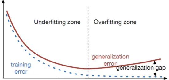
Generalization denotes how well a algorithm with learned parameters perform on unseen and independent and identically distributed (i.i.d) data compared to the training set, which is a crucial ability of the algorithm learning. The generalization error is defined as the expected loss on any new input.
To evaluate how good a model is, two factors are considered: 1. if the training error is small;
2. if the gap between training error and generalization error is small.
These two factors result in two important concepts in machine learning: un-derfitting and overfitting, which are highly related to the model capacity. As shown in Figure 1.1, underfitting occurs when the model does not have enough capacity to obtain a small training error while overfitting occurs when the model has enough capacity but the gap between training error and generalization error is large.
Figure 1.1 – The curve between training / generalization error and model capacity. X-axis denotes model capacity and Y-axis denotes the error.
1.2
Artificial Neural Networks
1.2.1
Perceptron
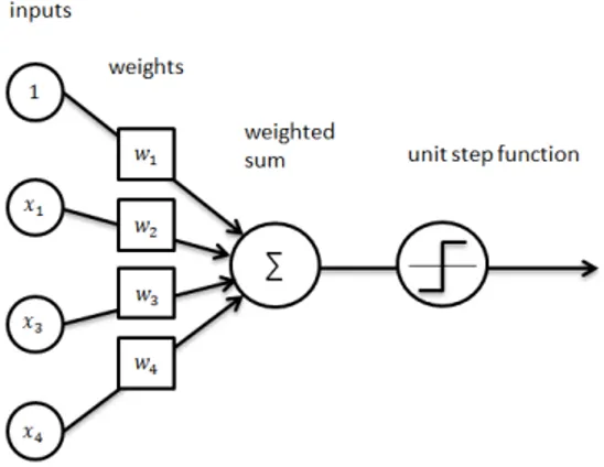
Inspired by the biological neural networks that build animal brains, Artificial Neural Networks (ANNs) are based on a collection of connected units called ar-tificial neurons, where each connection between neurons can transmit a signal to another neuron. One famous algorithm among ANNs dating back to early 60’s is Perceptron (Rosenblatt, 1958), which was created by Rosenblatt.
Perceptron is designed to tackle binary classification problem in supervise learn-ing. The algorithm is to learn to decide if an input belongs to a negative class or a positive class based on the dot product over a set of parameters and the input values. Formally, consider a set of inputs x = {x1, x2, ..., xd} containing d input
scalars, a set of d scalar weights w = {w1, w2, ..., wd} and a single scalar bias term
b, the perceptron algorithm is defined as follows:
f (x) = 8 < : 1 if w|x + b > 0 0 otherwise (1.5)
The bias term shifts the boundary from the origin and is independent of inputs. Figure 1.2 shows a schematic diagram of the algorithm.
Figure 1.2 – A graphical illustration of perceptron algorithm
The perceptron algorithm is also termed as single-layer perceptron, which is distinguished from multi-layer perceptron.
1.2.2
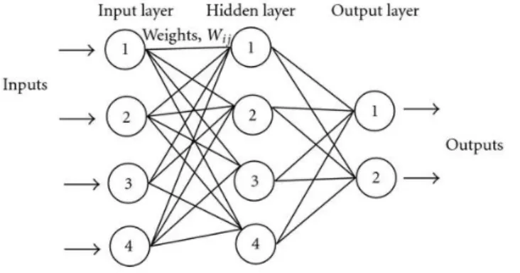
Multi-Layer Perceptrons
Multi-layer perceptron (MLP) is the extension of a single-layer perception, which consists of at least three layers (including an input layer and an output layer). Di↵erent from the unit step function used in perception algorithm, a non-linear activation function (which will be discussed in details in the following section) is applied to the dot product value.
Figure 1.3 – A graphical illustration of multi-layer perceptron
As shown in Figure 1.3, MLPs are fully connected. Each node in one layer is connected with a set of weights wijto every node in the following layer. Cybenko’s
theorem (Cybenko, 1989) shows that MLPs are universal function approximators, which proves that a 3-layer perceptron can approximate continuous functions on compact subsets of Rnunder certain assumptions. The property suggests that such
artificial neural networks could model various functions with appropriate weights and activation function. MLPs has been widely used in image classification (LeCun et al.,1998;Cire¸san et al.,2012) and speech recognition (Lopes and Perdigao,2011;
Bourlard and Morgan, 1990) since 1980’s.
1.2.3
Activation Function
The activation function is a crucial component in neural networks. It takes as input the dot product value with a bias term and output a value decides whether the node should be ”fired” or not. Here, we introduce several popular activation functions. In all the following functions, x, w, b represent an input random variable, a scalar weight and a scalar bias term, respectively.
• Unit step function is a discontinuous function that is used in perception algorithm. It it defined as:
f (x) = 8 < : 1 if x > 0 0 otherwise (1.6)
• Sigmoid function is inspired from probability theory and its output ranges from 0 to 1 in an ”S” shape, which is commonly used in multi-layer perceptron. It is defined as:
f (x) = 1
1 + e x (1.7)
• Hyperbolic tangent function (Tanh) is a rescaling of the sigmoid function in which output ranges from 1 to 1:
tanh x = sinh x cosh x =
ex e x
ex+ e x (1.8)
• Rectifier Linear Unit (ReLU) is inspired from biological motivations. The advantages of ReLU include efficient computation, sparse activation, etc. It is favored for deep neural networks:
f (x) = max(0, x) (1.9)
• Parametric Rectifier Linear Unit (PReLU) is an extension of the ReLU in which the output of the function in the regions that input is a linear function of the input with a slope of ↵:
f (x) = 8 < : f (x), if f (x) > 0 ↵f (x), otherwise (1.10)
the extra parameter ↵ is usually initialized to 0.1 and can be trained.
• Maxout takes the maximum output from n piece-wise linear functions: f (x) = max(f0(x), f00(x)) (1.11)
where for f’(x) and f”(x) we have:
f0(x) = w0⇥ x + b0, ... fn(x) = wn⇥ x + b00, (1.12)
• Softmax function is also named normalized exponential function. It nor-malizes K-dimensional vector x to a vector ranging from 0 to 1 that adds up to 1. It commonly used for represent a probability distribution for K possible outputs. Thus, softmax function has been highly used in classification tasks. It is defined as: (x)i = exi PK k=1exk (1.13)
1.2.4
Cost Functions
Following what we discussed about empirical risk in 1.1.3, it is necessary to define the concrete formulation of the cost function (also known as the objective function) L(ˆy, y), where ˆy is the prediction and y is the target. Typically, the output of the cost function is a measurement of how far the predictions are from the targets. Various cost functions could be chosen for specific tasks. Here, we introduce 3 popular cost functions:
Cross-Entropy: Cross-Entropy defines a loss between the categorical output and the target in a supervised classification model. The categorical output is usually interpreted as a probability value for its category from the softmax output:
L(ˆy, y) = X
c
1y=clog ˆyc (1.14)
where c denotes the target. The loss increases when the prediction diverges from the target and goes to zero when the prediction assigns 100% probability to the target class.
Mean Squared Error (MSE): Mean squared error has been widely use in regression tasks. Di↵erent from classification, regression models output continuous values: L(ˆy, y) = 1 n n X i=1 (ˆyi yi)2 (1.15)
where n denotes n training examples we could access.
target: L(ˆy, y) = 1 n n X i=1 |ˆyi yi| (1.16)
L1 loss function is robust and less vulnerable by outliers while MSE is very sensitive to outliers.
1.2.5
Optimization
In the deep learning context, optimization is defined as finding the optimal weights of a model that could minimize a given cost function. Optimization of ANNs is crucial and difficult. A set of approaches have been developed to solve the task and all popular optimizers methods are gradient-based.
One popular technique in gradient-based optimization family is gradient de-scent, which finds a local minimum of the given cost function based on the deriva-tives in a iterative way.
Suppose we have a model to learn a mapping function from x 2 X to y 2 Y ,
y = F (x; ✓), (1.17)
where ✓ is a set of learnable parameters. The derivative of the function in terms of parameters is defined as F✓0(x; ✓), which in 1-D, is the slope of F (x; ✓) with ✓ at the point x. It tells us how to scale ✓ to make an improvement over y. More specifically, we could reduce the value of loss function by changing the parameters as follows:
✓t+1= ✓t ✏F
0
✓(x; ✓t) (1.18)
where t indicates the t-th iteration and ✏ denotes a positive scalar determining the size of the step. The iteration would stop when y is lower than all the neighboring points.
To train the ANN parameters, we need to use gradient descent for backward propagation of errors (backpropagation) through di↵erent layers. The method com-putes the gradient of the cost function with respect to the parameters. In order to complete backpropagation, we need to use the chain rule. Suppose we have two
simple functions,
f (q, z) = q⇥ z (1.19)
q(x, y) = x + y (1.20)
we have known how to compute the gradient of f with respect to q and the gradient of q with respect to x from the aforementioned method. To compute the gradient of f with respect to x, we preform,
fx0(q, z) = fq0(q, z)⇥ qx0(x, y) (1.21) In this case, the gradient is simply obtained by multiplication of two gradient in each function.
Typically, a training dataset would be provided when we train ANNs. There are two trends to apply gradient descent: batch gradient descent (BGD) and stochastic gradient descent (SGD). Batch gradient descent calculates the gradient using the whole training dataset. This method could be expensive and inefficient when the dataset is in the large-scale. Stochastic gradient descent computes the gradient using a single example in the dataset, many applications of SGD actually use a mini-batch including several examples. The gradient computed in this case is noiser but it turns out working well. A graphical depiction of the di↵erence between BGD and SGD is shown in Figure1.4.
Figure 1.4 – A graphical depiction of the di↵erence between BGD and SGD. SGD o↵ers noiser gradient in each iteration.
One could image that standard SGD may oscillate across the ravine instead of going down to the optimum if the loss surface has the form of a long shallow ravine leading to the optimum and steep walls on the sides. In this case, standard SGD
may lead to slower convergence. Momentum (Sutskever et al., 2013) was proposed to alleviate this problem. The momentum update follows:
vt+1 = ↵vt+ ✏F
0
✓(x; ✓t) (1.22)
✓t+1 = ✓t vt+1 (1.23)
where vt+1 denotes the velocity at t + 1-th iteration, ↵ determines for how many
iterations from the previous gradients are involved into the current update.
SGD or SGD with momentum could be categorized as the first-order itera-tive optimization algorithm. Another popular first-order optimization algorithm is Adaptive Moment Estimation (Adam) proposed by Kingma and Ba in 2014 (Kingma and Ba, 2014) which computes the adaptive learning rates for each pa-rameter. It takes advantage of per-parameter learning rates that helps to improve the performance of the problems with sparse gradients and that are adapted based on the average of recent magnitudes of the gradients for the parameters. In addi-tion, Adam also benefit from the average of the second moments of the gradients. Basically, the algorithm computes an exponential moving average of the gradient and the squared gradient. There are two scalar hyper-parameters that control the decay rates of these moving averages. The detailed algorithm is described in Figure
1.5.
In addition to first-order optimization algorithms, second-order optimization has been explored as well. One simple instantiation is Newton’s method. Newton’s method is based on a second-order Taylor series expansion to approximate f(x) near some point x. Newton’s method could be helpful when the nearby point is a local minimum. In this case, it performs faster than gradient descent since it uses information about the second derivative which makes the convergence in fewer steps than gradient descent.
As we mentioned, optimization of ANNs can be difficult. One scenario is when the parameters get stuck at points that are neither maximum or minimum, we call these points as saddle points. A saddle point is the point where the derivatives become zero but not a local extremum on both axes. Research on how to escape saddle points when training ANNs has been developed in recent years (Dauphin et al., 2014;Jin et al., 2017).
2
Sequence to Sequence
Learning
In this chapter we will introduce several building blocks of sequence to sequence learning in deep learning scenarios – recurrent neural networks (RNNs), convolu-tional neural networks (CNNs) based sequence modelling and their variants.
2.1
Concept
Sequence to sequence learning typically denotes the methods to map the in-put sequence to a variable length outin-put sequence. More specifically, sequence to sequence learning includes synced sequence input to sequence output (labels are assigned to each unit of sequence input) and unsynced sequence input to sequence output (labels are not aligned with input). They has been successfully used in the domain of speech recognition (Graves et al., 2013; Graves and Jaitly, 2014; Sak et al., 2014), machine translation (Luong et al., 2015; Bahdanau et al., 2014) and optical character recognition (OCR) (Lee and Osindero, 2016; He et al., 2016d). The length of input for sequence to sequence learning is usually unknown as a pri-ori which would make MLPs fail easily. MLPs are powerful for the tasks whose inputs and outputs are of a fixed size, however, many problems have sequential properties. In the next section, we will present recurrent neural networks (RNNs), a class of ANNs whose connections between units are cyclic. The nature of RNNs allows them to model the temporal relations inside the sequential input.
2.2
Recurrent Neural Networks
Reccurent Neural Networks (RNNs) are sequential extension of feedforward neural networks. Given an input sequence of vectors (x1, . . . , xT ), the model
produces a sequence of hidden states (s1, . . . , sT) and a sequence of outputs (y1,
. . . , yT), which are computed at time step t as follows
st= '(Wst 1+ Uxt) (2.1)
ot= Vst (2.2)
where W is the recurrent weight matrix, U is the input-to-hidden weight matrix, V is the hidden-to-output weight matrix and ' is an arbitrary activation function (usually a logistic sigmoid function or tanh function). The parameters are shared by all time steps in the network.
The RNNs could map sequences to sequences with known alignment between the inputs and outputs. We show an unrolled recurrent neural network in Figure
2.1.
Figure 2.1 – A recurrent neural network unrolled in time (Figure adapted from Yoshua Bengio’s slides)
Training a recurrent neural network is similar to training MLPs. However, the gradient at each output depends not only on the current time step, but also the previous time steps, we call it backpropagation through time (BPTT). Training such networks via BPTT is known to be particularly difficult due to what is called the vanishing and exploding gradient problem, which hinders the models from learning long-term dependencies. The gradient @st
@st n can be computed as follows, @st @st n = t Y k=t n+1 UTdiag('0k), (2.3)
flow through time heavily depends on the hidden-to-hidden matrix U, but W and xtappear to play a limited role: they only come in the derivative of '0 mixed with
U. An improved architecture that efficiently utilize the information from di↵erent resources is proposed by Wu, et al in (Wu et al., 2016).
2.3
Long Short Term Memory
Long Short Term Memory (LSTM) is a special kind of recurrent structure which was proposed by Sepp Hochreiter and J¨urgen Schmidhuber in 1997 (Hochreiter and Schmidhuber,1997). It addresses the vanishing gradient problem commonly found in RNNs by incorporating gating functions into its state dynamics. The main components include a memory cell to store the state for the time step up to now, an input gate to modulate the extent to which a new input at time step t flows into the memory cell, an output gate to control the extent to which the information in the cell flows out, a forget gate to determine how much history would be preserved in the cell. More specifically, we define the computation at time step t as follows:
it= '(Wsist 1+ Uxixt) (2.4)
ft = '(Wsfst 1+ Uxfxt) (2.5)
ot= '(Wsost 1+ Uxoxt) (2.6)
ct= ft ct 1+ it (Wsst 1+ Uxcxt) (2.7)
st= ot '(ct) (2.8)
where it, ft, ot, ct, st denotes input gate, forget gate, output gate, memory cell
state and output of the LSTM unit, respectively. Ws. and Ux. are weight matrices
and denotes Hadamard product (element-wise product).
Variants to LSTM includes peephole LSTM whose gates are computed based on the memory cell state ct 1 and the input xt, convolutional LSTM which
incor-porates convolution operator that we will introduce in the following section. Gated recurrent unit (GRU) (Cho et al.,2014) is another gating mechanism which is sim-ilar to LSTM while there is only single gating unit determines the forgetting factor
and the extent to update the state. Empirical comparisons between LSTM and GRU can be found in (Chung et al.,2014).
2.4
Bidirectional Structure
Bidirectional RNNs were proposed by Schuster and Paliwal in 1997 (Schuster and Paliwal, 1997). They use information not only from the past states but also from the future states, which can access long-range context in both directions. Bidirectional structures has been shown to be superior over unidirectional structure in Graves and Schmidhuber (2005). A diagram depicting the di↵erence between two structures is shown in Figure 2.2.
Figure 2.2 – The di↵erence between a bidirectional RNN and an unidirectional RNN. (Figure adapted from wikipedia)
2.5
Convolutional Neural Networks
Convolutional neural networks (CNNs) is known as a class of feed-forward ANNs which were inspired by biological processes. They are widely used in the vision community for image classification, video recognition and other applications. CNNs
Figure 2.3 – The convolution layer and max-pooling layer applied upon input features.
have been popular for sequence modelling in recent years (Venugopalan et al.,
2015;Gehring et al.,2017) because of their computation efficiency and capacity to model long-range dependencies by stacking layers. A complete CNN is typically composed of stacked convolutional layers and pooling layers and at the top of which are multiple fully-connected layers. We introduce the building blocks of CNNs by taking acoustic features as input.
2.5.1
Convolution
As shown in Figure 2.3, given a sequence of input feature values X 2 Rc⇥b⇥f
with number of channels c, frequency bandwidth b, and time length f , the con-volutional layer convolves X with k filters {Wi}k where each Wi 2 Rc⇥m⇥n is a
3D tensor with its width along the frequency axis equal to m and its length along frame axis equal to n. The resulting k pre-activation feature maps consist of a 3D tensor H2 Rk⇥bH⇥fH, in which each feature map H
i is computed as follows:
Hi = Wi⇤ X + bi, i = 1,· · · , k. (2.9)
The symbol ⇤ denotes the convolution operation and bi is a bias parameter.
Convolution helps to extract features from input feature without losing spatial relations between units of the input. The size of the resulting feature maps is determined by the number of filters, the number of units by which the filters are slid (also known as stride) and the amount of padding around the border of the input (usually zero-padding). Each unit in the feature map is related to a local region of the input is known as receptive field. Another critical concept in CNNs
Figure 2.4 – Diliated convolution on 2D data. Figure is adapted fromYu and Koltun(2015)
is parameter sharing, which is used to control the number of parameters and to capture local features that could lie anywhere in the input.
Convolution has evolved into di↵erent variations in recent years. One popular variation is dilated convolution (Yu and Koltun,2015), which is a convolution with a dilated filter (Digram is shown in Figure2.4). Dilation factor could be customized depending on the task. Dilated convolution has been widely applied to semantic segmentation and audio generation (Yu and Koltun, 2015; Oord et al., 2016).
2.5.2
Pooling
After the element-wise non-linearities are applied to the pre-activation feature maps, the features will pass through a pooling layer which outputs the value from p adjacent units. The pooling operation reduces the dimensionality of the input while retaining the important local features. Pooling operations fall into various categories, such as mean pooling (mean value is computed over a region), max pooling (max value is computed over a region) and etc. In the case of max pooling, suppose that the i th feature map before and after pooling are ˜Hi and ˆHi, then
[ ˆHi]r,t at position (r, t) is computed by:
where s is the step size and p is the pooling size, and all the [ ˜Hi]r⇥s+j,t values
inside the max have the same time index t. Pooling operation results in translation invariant features, which means the same (pooled) feature will be active even when the image undergoes (small) translations. This property is desirable when the tasks are position independent, for example, object recognition.
2.5.3
Fully Connected Layer
A fully connected layer (FCL) is typically a set of MLP layers with a softmax function at the top. The purpose of FCL is to combine the local features from convolutional layers and pooling layers in a non-linear fashion. FCL is important when the global feature is needed for the task, for example, image classification. In sequence-to-sequence learning tasks, FCL is usually replaced by 1x1 convolution to keep the sequential nature. We refer readers to (Gehring et al., 2017) for more details.
2.6
Sequence Loss Function
Loss function design in unsynced sequence to sequence learning (labels are not aligned with input) is nontrivial due to its to-one, one-to-many or many-to-many mapping possibilities. We introduce a novel loss function, Connectionist Temporal Classification (CTC), which is proposed by Graves, et al (Graves et al.,
2006) that solves the many-to-one mapping problem in unsegmented sequence data.
2.6.1
Connectionist Temporal Classification
Consider any sequence to sequence mapping task in which X = {X1, ..., XT}
is the input sequence and Z = {Z1,· · · , ZL} is the target sequence. In the case
of speech recognition, X is the acoustic signal and Z is a sequence of symbols. In order to train the neural acoustic model, P r(Z|X) must be maximized for each input-output pair.
One way to provide a distribution over variable length output sequences given some much longer input sequence, is to introduce a many-to-one mapping of latent
variable sequences O = {O1,· · · , OT} to shorter sequences that serve as the final
predictions. The probability of some sequence Z can then be defined to be the sum of the probabilities of all the latent sequences that map to that sequence. Connec-tionist Temporal Classification (CTC) (Graves et al., 2006) specifies a distribution over latent sequences by applying a softmax function to the output of the network for every time step, which provides a probability for emitting each label from the alphabet of output symbols at that time step P r(Ot|X). An extra blank output
class ‘-’ is introduced to the alphabet for the latent sequences to represent the prob-ability of not outputting a symbol at a particular time step. Each latent sequence sampled from this distribution can now be transformed into an output sequence using the many-to-one mapping function (·) which first merges the repetitions of consecutive non-blank labels to a single label and subsequently removes the blank labels as shown in Equation 2.11:
(a, b, c, , ) (a, b, , c, c) (a, a, b, b, c) ( , a, , b, c) ... ( , , a, b, c) 9 > > > > > > > > > = > > > > > > > > > ; = (a, b, c). (2.11)
Therefore, the final output sequence probability is a summation over all possible sequences ⇡ that yield to Z after applying the function :
P r(Z|X) = ⌃o2 1(Z)P r(O|X). (2.12) A dynamic programming algorithm similar to the forward algorithm for HMMs
Graves (2012b) is used to compute the sum in Equation 2.12 in an efficient way. The intermediate values of this dynamic programming can also be used to compute the gradient of ln P r(Z|X) with respect to the neural network outputs efficiently.
To generate predictions from a trained model using CTC, we use the best path decoding algorithm. Since the model assumes that the latent symbols are indepen-dent given the network outputs in the framewise case, the latent sequence with the highest probability is simply obtained by emitting the most probable label at each time-step. The predicted sequence is then given by applying (·) to that latent
sequence prediction:
L⇡ (⇡⇤), (2.13)
in which ⇡⇤ is the concatenation of the most probable output and is formalized
by ⇡⇤ = Argmax
⇡P r(⇡|X). Note that this is not necessarily the output sequence
with the highest probability. Finding this sequence is generally not tractable and requires some approximate search procedure like a beam-search.
In the following chapters, we present two new approaches of sequence-to-sequence modelling on speech. The first one is based on CNNs and the other is built on RNNs.
3
Prologue to First Article
Towards End-to-End Speech Recognition with Deep Convolutional Neural Networks. Ying Zhang, Mohammad Pezeshki, Phil´emon Brakel, Saizheng Zhang, C´esar Laurent Yoshua Bengio, Aaron Courville. Interspeech, 2016.
Personal Contribution. The underlying idea of combining convolutional neu-ral networks with connectionist temponeu-ral classification was mine. Mohammad Pezeshki, Phil´emon Brakel and I discussed the structure variations based on the model. I conducted the experiments on TIMIT and Mohammad worked on Wall Street Journal. I implemented the majority of the code based on our private speech repository in MILA. I contributed to the writing of the paper while Mohammad Pezeshki, Phil´emon Brakel, Saizheng Zhang and C´esar Laurent helped to revise the paper, with valuable comments from my supervisors Aaron Courville and Yoshua Bengio.
4
Towards End-to-End Speech
Recognition with Deep
Convolutional Neural
Networks
4.1
Introduction
Recently, Convolutional Neural Networks (CNNs) (LeCun et al., 1998) have achieved great success in acoustic modeling (Abdel-Hamid et al., 2012; Sainath et al., 2013b,a). In the context of Automatic Speech Recognition, CNNs are usu-ally combined with HMMs/GMMs (Mohamed et al.,2012;Hinton et al.,2012), like regular Deep Neural Networks (DNNs), which results in a hybrid system ( Abdel-Hamid et al., 2012; Sainath et al., 2013b,a). In the typical hybrid system, the neural net is trained to predict frame-level targets obtained from a forced align-ment generated by an HMM/GMM system. The temporal modeling and decoding operations are still handled by an HMM but the posterior state predictions are generated using the neural network.
This hybrid approach is problematic in that training the di↵erent modules sep-arately with di↵erent criteria may not be optimal for solving the final task. As a consequence, it often requires additional hyperparameter tuning for each train-ing stage which can be laborious and time consumtrain-ing. Furthermore, these issues have motivated a recent surge of interests in training ‘end-to-end’ systems (Hannun et al., 2014; Bahdanau et al.,2016; Miao et al., 2015). End-to-end neural systems for speech recognition typically replace the HMM with a neural network that pro-vides a distribution over sequences directly. Two popular neural network sequence models are Connectionist Temporal Classification (CTC) (Graves et al.,2006) and recurrent models for sequence generation (Bahdanau et al.,2016;Chorowski et al.,
2015).
To the best of our knowledge, all end-to-end neural speech recognition systems employ recurrent neural networks in at least some part of the processing pipeline. The most successful recurrent neural network architecture used in this context is the Long Short-Term Memory (LSTM) (Graves et al.,2013;Graves,2012a;Hochreiter
and Schmidhuber,1997; Vinyals et al.,2012). For example, a model with multiple layers of bi-directional LSTMs and CTC on top which is pre-trained with the transducer networks (Graves et al.,2013;Graves,2012a) obtained the state-of-the-art on the TIMIT dataset. After these successes on phoneme recognition, similar systems have been proposed in which multiple layers of RNNs were combined with CTC to perform large vocabulary continuous speech recognition (Hannun et al.,
2014; Miao et al., 2013). It seems that RNNs have become somewhat of a default method for end-to-end models while hybrid systems still tend to rely on feed-forward architectures.
While the results of these RNN-based end-to-end systems are impressive, there are two important downsides to using RNNs/LSTMs: (1) The training speed can be very slow due to the iterative multiplications over time when the input sequence is very long; (2) The training process is sometimes tricky due to the well-known problem of gradient vanishing/exploding (Hochreiter, 1991; Bengio et al., 1994). Although various approaches have been proposed to address these issues, such as data/model parallelization across multiple GPUs (Hannun et al., 2014; Sutskever et al., 2014) and careful initializations for recurrent connections (Le et al., 2015), those models still su↵er from computationally intensive and otherwise demanding training procedures.
Inspired by the strengths of both CNNs and CTC, we propose an end-to-end speech framework in which we combine CNNs with CTC without intermediate recurrent layers. We present experiments on the TIMIT dataset and show that such a system is able to obtain results that are comparable to those obtained with multiple layers of LSTMs. The only previous attempt to combine CNNs with CTC that we know about (Song and Cai), led to results that were far from the state-of-the-art. It is not straightforward to incorporate CNN into an end-to-end manner since the task may require the model to incorporate long-term dependencies. While RNNs can learn these kind of dependencies and have been combined with CTC for this very reason, it was not known whether CNNs were able to learn the required temporal relationships.
In this paper, we argue that in a CNN of sufficient depth, the higher-layer features are capable of capturing temporal dependencies with suitable context in-formation. Using small filter sizes along the spectrogram frequency axis, the model is able to learn fine-grained localized features, while multiple stacked convolutional
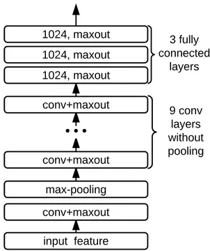
input feature conv+maxout max-pooling conv+maxout 9 conv layers without pooling conv+maxout 1024, maxout 1024, maxout 1024, maxout 3 fully connected layers
Figure 4.1 – Network structure for phoneme recognition on the TIMIT dataset. The model consists of 10 convolutional layers followed by 3 fully-connected layers on the top. All convolutional layers have the filter size of 3⇥ 5 and we use max-pooling with size of 3 ⇥ 1 only after the first convolutional layer. First and second numbers correspond to frequency and time axes respectively.
layers help to learn diverse features on di↵erent time/frequency scales and provide the required non-linear modeling capabilities.
Unlike the time windows applied in DNN systems (Abdel-Hamid et al., 2012;
Sainath et al., 2013b,a), the temporal modeling is deployed within convolutional layers, where we perform a 2D convolution similar to vision tasks, and multiple convolutional layers are stacked to provide a relatively large context window for each output prediction of the highest layer. The convolutional layers are followed by multiple fully connected layers and, finally, CTC is added on the top of the model. Following the suggestion from (Sainath et al., 2013a), we only perform pooling along the frequency band on the first convolutional layer. Specifically, we evaluate our model on phoneme recognition for the TIMIT dataset.
4.2
Experiments
In this section, we evaluate the proposed model on phoneme recognition for the TIMIT dataset. The model architecture is shown in Figure 4.1.
4.2.1
Data
We evaluate our models on the TIMIT (Garofolo et al., 1993) corpus where we use the standard 462-speaker training set with all SA records removed. The 50-speaker development set is used for early stopping. The evaluation is performed on the core test set (including 192 sentences). The raw audio is transformed into 40-dimensional log mel-filter-bank (plus energy term) coefficients with deltas and delta-deltas, which results in 123 dimensional features. Each dimension is normal-ized to have zero mean and unit variance over the training set. We use 61 phone labels plus a blank label for training and then the output is mapped to 39 phonemes for scoring.
4.2.2
Models
Our best model consists of 10 convolutional layers and 3 fully-connected hidden layers. Unlike the other layers, the first convolutional layer is followed by a pooling layer, which is described in section 2. The pooling size is 3⇥ 1, which means we only pool over the frequency axis. The filter size is 3⇥ 5 across the layers. The model has 128 feature maps in the first four convolutional layers and 256 feature maps in the remaining six convolutional layers. Each fully-connected layer has 1024 units. Maxout with 2 piece-wise linear functions is used as the activation function. Some other architectures are also evaluated for comparison, see section 4.4 for more details.
4.2.3
Training and Evaluation
To optimize the model, we use Adam (Kingma and Ba, 2014) with learning rate 10 4. Stochastic gradient descent with learning rate 10 5 is then used for
fine-tuning. Batch size 20 is used during training. The initial weight values were drawn uniformly from the interval [ 0.05, 0.05]. Dropout (Srivastava et al.,2014) with a probability of 0.3 is added across the layers except for the input and output
layers . L2 norm with coefficient 1e 5 is applied at fine-tuning stage. At test time, simple best path decoding (at the CTC frame level) is used to get the predicted sequences.
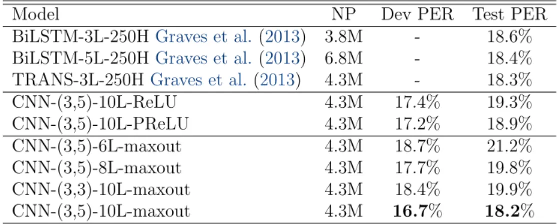
4.2.4
Results
Our model achieves 18.2% phoneme error rate on the core test set, which is slightly better than the LSTM baseline model and the transducer model with an explicit RNN language model. The details are presented in Table 4.1. Notice that the CNN model could take much less time to train in comparison with the LSTM model when keeping roughly the same number of parameters. In our setup on TIMIT, we get 2.5⇥ faster training speed by using the CNN model without deliberately optimizing the implementation. We suppose that the gain of the com-putation efficiency might be more dramatic with a larger dataset.
To further investigate the di↵erent structural aspects of our model, we disentan-gle the analysis into three sub-experiments considering the number of convolutional layers, the filter sizes and the activation functions, as shown in table 4.1. It turns out that the model may benefit from (1) more layers, which results in more nonlin-earities and larger input receptive fields for units in the top layers; (2) reasonably large context windows, which help the model to capture the spatial/temporal rela-tions of input sequences in reasonable time-scales; (3) the Maxout unit, which has more functional freedoms comparing to ReLU and parametric ReLU.
4.3
Discussion
Our results showed that convolutional architectures with CTC cost can achieve results comparable to the state-of-the-art by adopting the following methodology: (1) Using a significantly deeper architecture that results in a more non-linear func-tion and also wider receptive fields along both frequency and temporal axes; (2) Using maxout non-linearities in order to make the optimization easier; and (3) Careful model regularization that yields better generalization in test time, espe-cially for small datasets such as TIMIT, where over-fitting happens easily.
Table 4.1 – Phoneme Error Rate (PER) on TIMIT. ’NP’ is the number of parameters. ’BiLSTM-3L-250H’ denotes the model has 3 bidirectional LSTM layers with 250 units in each direction. In the CNN model, (3, 5) is the filter size. Results suggest that deeper architecture and larger filter sizes leads to better performance. The best performing model on Development set, has a test PER of 18.2 %
Model NP Dev PER Test PER
BiLSTM-3L-250HGraves et al. (2013) 3.8M - 18.6% BiLSTM-5L-250HGraves et al. (2013) 6.8M - 18.4% TRANS-3L-250HGraves et al. (2013) 4.3M - 18.3%
CNN-(3,5)-10L-ReLU 4.3M 17.4% 19.3% CNN-(3,5)-10L-PReLU 4.3M 17.2% 18.9% CNN-(3,5)-6L-maxout 4.3M 18.7% 21.2% CNN-(3,5)-8L-maxout 4.3M 17.7% 19.8% CNN-(3,3)-10L-maxout 4.3M 18.4% 19.9% CNN-(3,5)-10L-maxout 4.3M 16.7% 18.2%
We conjecture that the convolutional CTC model might be easier to train on phoneme-level sequences rather than the character-level. Our intuition is that the local structures within the phonemes are more robust and can easily be captured by the model. Additionally, phoneme-level training might not require the modeling of many long-term dependencies in comparison with character-level training. As a result, for a convolutional model, learning the phonemes structure seems to be easier, but empirical research needs to be done to investigate if this is indeed the case.
Finally, an important point that favors convolutional over recurrent architec-tures is the training speed. In a CNN, the training time can be rendered virtually independent of the length of the input sequence due to the parallel nature of con-volutional models and the highly optimized CNN libraries available (Abadi et al.,
2016). Computations in a recurrent model are sequential and cannot be easily par-allelized. The training time for RNNs increases at least linearly with the length of the input sequence.
5
Prologue to Second Article
Deep Complex Networks. Chiheb Trabelsi1, Olexa Bilaniuk1, Ying Zhang,
Dmitriy Serdyuk, Sandeep Subramanian, Jo˜ao Felipe Santos, Soroush Mehri, Negar Rostamzadeh, Yoshua Bengio, Christopher J.Pal. Sixth International Conference on Learning Representations (ICLR), 2018.
Personal Contribution. Chiheb Trabelsi and I proposed the idea of recurrent complex networks. I prepared the code for recurrent models with audio data, conducted the spectrum experiments and wrote the paper on that section. The rest of the authors worked on the feed-foward nets.
6
Deep Complex Networks
6.1
Introduction
Recent research advances have made significant progress in addressing the dif-ficulties involved in learning deep neural network architectures. Key innovations include normalization techniques (Io↵e and Szegedy, 2015; Salimans and Kingma,
2016) and the emergence of gating-based feed-forward neural networks like High-way Networks (Srivastava et al.,2015). Residual networks (He et al.,2016b,c) have emerged as one of the most popular and e↵ective strategies for training very deep convolutional neural networks (CNNs). Both highway networks and residual net-works facilitate the training of deep netnet-works by providing shortcut paths for easy gradient flow to lower network layers thereby diminishing the e↵ects of vanishing gradients (Hochreiter,1991). He et al.(2016c) show that learning explicit residuals of layers helps in avoiding the vanishing gradient problem and provides the network with an easier optimization problem. Batch normalization (Io↵e and Szegedy,2015) demonstrates that standardizing the activations of intermediate layers in a network across a minibatch acts as a powerful regularizer as well as providing faster training and better convergence properties. Further, such techniques that standardize layer outputs become critical in deep architectures due to the vanishing and exploding gradient problems.
The role of representations based on complex numbers has started to receive in-creased attention, due to their potential to enable easier optimization (Nitta,2002), better generalization characteristics (Hirose and Yoshida, 2012), faster learning (Arjovsky et al., 2016; Danihelka et al., 2016; Wisdom et al., 2016) and to al-low for noise-robust memory mechanisms (Danihelka et al., 2016). Wisdom et al.
(2016) and Arjovsky et al. (2016) show that using complex numbers in recurrent neural networks (RNNs) allows the network to have a richer representational ca-pacity. Danihelka et al. (2016) present an LSTM (Hochreiter and Schmidhuber,
1997) architecture augmented with associative memory with complex-valued inter-nal representations. Their work highlights the advantages of using complex-valued representations with respect to retrieval and insertion into an associative memory. In residual networks, the output of each block is added to the output history ac-cumulated by summation until that point. An efficient retrieval mechanism could help to extract useful information and process it within the block.
In order to exploit the advantages o↵ered by complex representations, we present a general formulation for the building components of complex-valued deep neural networks and apply it to the context of feed-forward convolutional networks and convolutional LSTMs. Our contributions in this paper are as follows:
1. A formulation of complex batch normalization, which is described in Section6.2.5;
2. Complex weight initialization, which is presented in Section 6.2.6;
3. A comparison of di↵erent complex-valued ReLU-based activation functions presented in Section 6.3.1;
4. A state of the art result on the MusicNet multi-instrument music transcription dataset, presented in Section 6.3.2;
5. A state of the art result in the Speech Spectrum Prediction task on the TIMIT dataset, presented in Section6.3.3.
We perform a sanity check of our deep complex network and demonstrate its e↵ectiveness on standard image classification benchmarks, specifically, CIFAR-10, CIFAR-100. We also use a reduced-training set of SVHN that we call SVHN*. For
audio-related tasks, we perform a music transcription task on the MusicNet dataset and a Speech Spectrum prediction task on TIMIT. The results obtained for vision classification tasks show that learning complex-valued representations results in performance that is competitive with the respective real-valued architectures. Our promising results in music transcription and speech spectrum prediction underscore the potential of deep complex-valued neural networks applied to acoustic related tasks1 – We continue this paper with discussion of motivation for using complex operations and related work.
1. The source code is located at http://github.com/ChihebTrabelsi/deep_complex_ networks
6.2
Complex Building Blocks
In this section, we present the core of our work, laying down the mathemati-cal framework for implementing complex-valued building blocks of a deep neural network.
6.2.1
Representation of Complex Numbers
We start by outlining the way in which complex numbers are represented in our framework. A complex number z = a + ib has a real component a and an imaginary component b. We represent the real part a and the imaginary part b of a complex number as logically distinct real valued entities and simulate complex arithmetic using real-valued arithmetic internally. Consider a typical real-valued 2D convolution layer that has N feature maps such that N is divisible by 2; to represent these as complex numbers, we allocate the first N/2 feature maps to represent the real components and the remaining N/2 to represent the imaginary ones. Thus, for a four dimensional weight tensor W that links Nin input feature
maps to Nout output feature maps and whose kernel size is m⇥ m we would have
a weight tensor of size (Nout⇥ Nin⇥ m ⇥ m) /2 complex weights.
6.2.2
Complex Convolution
In order to perform the equivalent of a traditional real-valued 2D convolution in the complex domain, we convolve a complex filter matrix W = A + iB by a complex vector h = x + iy where A and B are real matrices and x and y are real vectors since we are simulating complex arithmetic using real-valued entities. As the convolution operator is distributive, convolving the vector h by the filter W we obtain:
W⇤ h = (A ⇤ x B⇤ y) + i (B ⇤ x + A ⇤ y). (6.1) As illustrated in Figure 6.1a, if we use matrix notation to represent real and imag-inary parts of the convolution operation we have:
" <(W ⇤ h) =(W ⇤ h) # = " A B B A # ⇤ " x y # . (6.2)
(a) An illustration of the complex convolu-tion operator.
(b) A complex convolutional residual net-work (left) and an equivalent real-valued residual network (right).
Figure 6.1 – Complex convolution and residual network implementation details.
6.2.3
Complex Di↵erentiability
In order to perform backpropagation in a complex-valued neural network, a sufficient condition is to have a cost function and activations that are di↵erentiable with respect to the real and imaginary parts of each complex parameter in the network.
By constraining activation functions to be complex di↵erentiable or holomor-phic, we restrict the use of possible activation functions for a complex valued neural networks. Hirose and Yoshida (2012) shows that it is unnecessarily restrictive to limit oneself only to holomorphic activation functions; Those functions that are di↵erentiable with respect to the real part and the imaginary part of each pa-rameter are also compatible with backpropagation. (Arjovsky et al.,2016;Wisdom et al.,2016;Danihelka et al.,2016) have used non-holomorphic activation functions and optimized the network using regular, real-valued backpropagation to compute partial derivatives of the cost with respect to the real and imaginary parts.
Even though their use greatly restricts the set of potential activations, it is worth mentioning that holomorphic functions can be leveraged for computational efficiency purposes. As pointed out in Sarro↵ et al. (2015), using holomorphic functions allows one to share gradient values. So, instead of computing and back-propagating 4 di↵erent gradients, only 2 are required.
6.2.4
Complex-Valued Activations
ModReLU
Numerous activation functions have been proposed in the literature in order to deal with complex-valued representations. (Arjovsky et al., 2016) have proposed modReLU, which is defined as follows:
modReLU(z) = ReLU(|z| + b) ei✓z = 8 < : (|z| + b)z |z| if |z| + b 0, 0 otherwise, (6.3)
where z 2 C, ✓z is the phase of z, and b 2 R is a learnable parameter. As |z| is
always positive, a bias b is introduced in order to create a “dead zone” of radius b around the origin 0 where the neuron is inactive, and outside of which it is active. The authors have used modReLU in the context of unitary RNNs. Their design of modReLU is motivated by the fact that applying separate ReLUs on both real and imaginary parts of a neuron performs poorly on toy tasks. The intuition behind the design of modReLU is to preserve the pre-activated phase ✓z, as altering it with an
activation function severely impacts the complex-valued representation. modReLU does not satisfy the Cauchy-Riemann equations, and thus is not holomorphic. We have tested modReLU in deep feed-forward complex networks and the results are given in Table6.1.
CReLU and zReLU
We call Complex ReLU (or CReLU) the complex activation that applies sepa-rate ReLUs on both of the real and the imaginary part of a neuron, i.e:
CReLU satisfies the Cauchy-Riemann equations when both the real and imaginary parts are at the same time either strictly positive or strictly negative. This means that CReLU satisfies the Cauchy-Riemann equations when ✓z 2 ]0, ⇡/2[ or ✓z 2
]⇡, 3⇡/2[. We have tested CReLU in deep feed-forward neural networks and the results are given in Table6.1.
It is also worthwhile to mention the work done by Guberman (2016) where a ReLU-based complex activation which satisfies the Cauchy-Riemann equations everywhere except for the set of points{<(z) > 0, =(z) = 0}[{<(z) = 0, =(z) > 0} ias used. The activation function has similarities to CReLU. We call Guberman
(2016) activation as zReLU and is defined as follows:
zReLU(z) = 8 < : z if ✓z 2 [0, ⇡/2], 0 otherwise, (6.5)
We have tested zReLU in deep feed-forward complex networks and the results are given in Table6.1.
6.2.5
Complex Batch Normalization
Deep networks generally rely upon Batch Normalization (Io↵e and Szegedy,
2015) to accelerate learning. In some cases batch normalization is essential to optimize the model. The standard formulation of Batch Normalization applies only to real values. In this section, we propose a batch normalization formulation that can be applied for complex values.
To standardize an array of complex numbers to the standard normal complex distribution, it is not sufficient to translate and scale them such that their mean is 0 and their variance 1. This type of normalization does not ensure equal variance in both the real and imaginary components, and the resulting distribution is not guaranteed to be circular; It will be elliptical, potentially with high eccentricity.
We instead choose to treat this problem as one of whitening 2D vectors, which implies scaling the data by the square root of their variances along each of the two principal components. This can be done by multiplying the 0-centered data (x E[x]) by the inverse square root of the 2 ⇥ 2 covariance matrix V :
˜
where the covariance matrix V is V = Vrr Vri Vir Vii ! = Cov(<{x}, <{x}) Cov(<{x}, ={x}) Cov(={x}, <{x}) Cov(={x}, ={x}) ! .
The square root and inverse of 2⇥2 matrices has an inexpensive, analytical solution, and its existence is guaranteed by the positive (semi-)definiteness of V . Positive definiteness of V is ensured by the addition of ✏I to V (Tikhonov regularization). The mean subtraction and multiplication by the inverse square root of the variance ensures that ˜x has standard complex distribution with mean µ = 0, covariance = 1 and pseudo-covariance (also called relation) C = 0. The mean, the covariance and the pseudo-covariance are given by:
µ = E [˜x]
=E [(˜x µ) (˜x µ)⇤] = Vrr+ Vii+ i (Vir Vri)
C = E [(˜x µ) (˜x µ)] = Vrr Vii+ i (Vir+ Vri).
(6.6)
The normalization procedure allows one to decorrelate the imaginary and real parts of a unit. This has the advantage of avoiding co-adaptation between the two components which reduces the risk of overfitting (Cogswell et al., 2015; Srivastava et al., 2014).
Analogously to the real-valued batch normalization algorithm, we use two pa-rameters, and . The shift parameter is a complex parameter with two learn-able components (the real and imaginary means). The scaling parameter is a 2⇥ 2 positive semi-definite matrix with only three degrees of freedom, and thus only three learnable components. In much the same way that the matrix (V ) 12 normalized the variance of the input to 1 along both of its original principal compo-nents, so does scale the input along desired new principal components to achieve a desired variance. The scaling parameter is given by:
= rr ri
ri ii
! .
As the normalized input ˜x has real and imaginary variance 1, we initialize both
rr and ii to 1/
p
2 in order to obtain a modulus of 1 for the variance of the normalized value. ri, <{ } and ={ } are initialized to 0. The complex batch
normalization is defined as:
BN (˜x) = x + .˜ (6.7)
We use running averages with momentum to maintain an estimate of the complex batch normalization statistics during training and testing. The moving averages of Vri and are initialized to 0. The moving averages of Vrr and Vii are initialized to
1/p2. The momentum for the moving averages is set to 0.9.
6.2.6
Complex Weight Initialization
In a general case, particularly when batch normalization is not performed, proper initialization is critical in reducing the risks of vanishing or exploding gra-dients. To do this, we follow the same steps as in Glorot and Bengio (2010) and
He et al. (2015) to derive the variance of the complex weight parameters. A complex weight has a polar form as well as a rectangular form
W =|W |ei✓ =<{W } + i ={W }, (6.8)
where ✓ and |W | are respectively the argument (phase) and magnitude of W . Variance is the di↵erence between the expectation of the squared magnitude and the square of the expectation:
Var(W ) =E [W W⇤] (E [W ])2 =E⇥|W |2⇤ (E [W ])2,
which reduces, in the case of W symmetrically distributed around 0, to E [|W |2].
We do not know yet the value of Var(W ) =E [|W |2]. However, we do know a related
quantity, Var(|W |), because the magnitude of complex normal values, |W |, follows the Rayleigh distribution (Chi-distributed with two degrees of freedom (DOFs)). This quantity is
Var(|W |) = E [|W ||W |⇤] (E [|W |])2 =E⇥|W |2⇤ (E [|W |])2. (6.9) Putting them together:
We now have a formulation for the variance of W in terms of the variance and expectation of its magnitude, both properties analytically computable from the Rayleigh distribution’s single parameter, , indicating the mode. These are:
E [|W |] = r ⇡ 2, Var(|W |) = 4 ⇡ 2 2.
The variance of W can thus be expressed in terms of its generating Rayleigh dis-tribution’s single parameter, , thus:
Var(W ) = 4 ⇡ 2 2+ ✓ r ⇡ 2 ◆2 = 2 2. (6.10)
If we want to respect theGlorot and Bengio(2010) criterion which ensures that the variances of the input, the output and their gradients are the same, then we would have Var(W ) = 2/(nin+ nout), where nin and nout are the number of input
and output units respectively. In such case, = 1/pnin+ nout. If we want to
respect the He et al. (2015) initialization that presents an initialization criterion that is specific to ReLUs, then Var(W ) = 2/nin which = 1/pnin.
The magnitude of the complex parameter W is then initialized using the Rayleigh distribution with the appropriate mode . We can see from equation6.10, that the variance of W depends on on its magnitude and not on its phase. We then initialize the phase using the uniform distribution between ⇡ and ⇡. By performing the multiplication of the magnitude by the phasor as is detailed in equation 6.8, we perform the complete initialization of the complex parameter.
In all the experiments that we report, we use variant of this initialization which leverages the independence property of unitary matrices. As it is stated inCogswell et al.(2015),Srivastava et al.(2014), and Tompson et al.(2015), learning decorre-lated features is beneficial for learning as it allows to perform better generalization and faster learning. This motivates us to achieve initialization by considering a (semi-)unitary matrix which is reshaped to the size of the weight tensor. Once this is done, the weight tensor is mutiplied bypHevar/Var(W ) or
p
Glorotvar/Var(W )
where Glorotvar and Hevar are respectively equal to 2/(nin+ nout) and 2/nin. In
such a way we allow kernels to be independent from each other as much as pos-sible while respecting the desired criterion. Note that we perform the analogous initialization for real-valued models by leveraging the independence property of orthogonal matrices in order to build kernels that are as much independent from each other as possible while respecting a given criterion.