3D navigation based on a visual memory

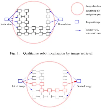
In the second method, the robot still converges to intermediary positions with an image-based visual servoing, but the current servoing is stopped as soon as enough points defining

The final chapter, “Sacred Art Today”, pays special attention to the presentation of various theories on the concept of sacred art, belonging to

means, including the scheduling of a technical presentation on the subject at the twenty-ninth session of the Regional Committee, at which time a report will

In this paper, we study the dependence of the buckling load of a non- shallow arch with respect to the shape of the midcurve.. The model we consider is the simple Eulerian buckling

In this model, CKI δ acts on the adjacent serine residues when Ser662 is phosphorylated (blue path in Fig. 1), but CKI δ also acts independently of Ser662 phosphory- lation

The IE approach emphasised the optimisation of resource flows by holding a system view that placed boundaries around the MW management system (Research 1), C&I and C&D

Various behavioral techniques have been employed and researched in terms of enhancing the social behavior of children with ASD such as: trial training, making use of stereotypic

With the vGATE method, we have identified and permanently tagged a small subpopulation of OT cells, which, by optogenetic stimulation, strongly attenuated