HAL Id: hal-01688108
https://hal.archives-ouvertes.fr/hal-01688108
Submitted on 7 Nov 2018
HAL is a multi-disciplinary open access
archive for the deposit and dissemination of
sci-entific research documents, whether they are
pub-lished or not. The documents may come from
teaching and research institutions in France or
abroad, or from public or private research centers.
L’archive ouverte pluridisciplinaire HAL, est
destinée au dépôt et à la diffusion de documents
scientifiques de niveau recherche, publiés ou non,
émanant des établissements d’enseignement et de
recherche français ou étrangers, des laboratoires
publics ou privés.
Null-collision meshless Monte-Carlo-Application to the
validation of fast radiative transfer solvers embedded in
combustion simulators
Vincent Eymet, Damien Poitou, M. Galtier, Mouna El-Hafi, Guillaume
Terrée, Richard Fournier
To cite this version:
Vincent Eymet, Damien Poitou, M. Galtier, Mouna El-Hafi, Guillaume Terrée, et al.. Null-collision
meshless Monte-Carlo-Application to the validation of fast radiative transfer solvers embedded in
combustion simulators. Journal of Quantitative Spectroscopy and Radiative Transfer, Elsevier, 2013,
129, pp.145-157. �10.1016/j.jqsrt.2013.06.004�. �hal-01688108�
Null-collision meshless Monte-Carlo—Application to the
validation of fast radiative transfer solvers embedded in
combustion simulators
V. Eymet
a,n, D. Poitou
a, M. Galtier
a, M. El Hafi
a, G. Terrée
a, R. Fournier
baUniversité de Toulouse; Mines Albi, CNRS, centre RAPSODEE; Campus Jarlard, F-81013 Albi cedex 09, France bLAPLACE, UMR 5213, Université Paul Sabatier, 118, Route de Narbonne, 31062 Toulouse Cedex, France
Keywords: Monte-Carlo Null-collision Meshless Heterogeneous media Integral formulation Combustion a b s t r a c t
The Monte-Carlo method is often presented as a reference method for radiative transfer simulation when dealing with participating, inhomogeneous media. The reason is that numerical uncertainties are only of a statistical nature and are accurately evaluated by measuring the standard deviation of the Monte Carlo weight. But classical Monte-Carlo algorithms first sample optical thicknesses and then determine absorption or scattering locations by inverting the formal integral definition of optical thickness as an increasing function of path length. This function is only seldom analytically invertible and numerical inversion procedures are required. Most commonly, a volumic grid is introduced and optical properties within each cell are replaced by approximate homogeneous or linear fields. Simulation results are then sensitive to the grid and can no longer be considered as references. We propose a new algorithmic formulation based on the use of null-collisions that eliminate the need for numerical inversion: no volumic grid is required. Benchmark configurations are first considered in order to evaluate the effect of two free parameters: the amount of null-collisions, and the criterion used to decide at which stage a Russian Roulette is used to exit the path tracking process. Then the corresponding algorithm is implemented using a development environment allowing to deal with complex geome-tries (thanks to computer graphics techniques), leading to a Monte Carlo code that can be easily used for validation of fast radiative transfer solvers embedded in combustion simulators. “Easily” means here that the way the Monte Carlo algorithm deals with both the geometry and the temperature/pressure/concentration fields is independent of the choices made inside the combustion solver: there is no need for the design of a new path-tracking procedure adapted to each new CFD grid. The Monte Carlo simulator is ready for use as soon as combustion specialists provide a localization/interpolation tool defining what they consider as the continuous input fields best suiting their numerical assump-tions. The radiation validation tool introduces no grid in itself.
1. Introduction
Industrial applications, such as combustion processes, require radiative transfer modeling, often coupled with other energy transfer mechanisms. Numerical radiative transfer solvers used in such applications need to reach the best compromise between numerical accuracy and
nCorresponding author.
E-mail addresses:[email protected], [email protected] (V. Eymet)
computation cost. These tools also need validation, and therefore reference numerical methods have to be used. The Monte-Carlo method (MCM) is known to be one of these reference methods. Like all other methods, MCM evaluates numerically the solution of the radiative transfer equation (RTE) and its “reference” status is only due to the existence of a rigorous measure of its uncertainty: from its statistical nature, MCM allows the systematic calculation of a standard deviation associated to each numerical result, and this standard deviation is translated into a numerical uncertainty thanks to the central limit theorem. However, designing Monte-Carlo algorithms to be used in complex geometries has long been a quite challenging task, mainly because of prohibitive computational costs. Using MCM to produce references and validate the radia-tive parts of heat-transfer or combustion solvers was therefore hardly feasible outside academic configurations. Recent developments, such as the work reported by Zhang et al. [1,2], show that this is now practically feasible whatever the complexity of industrial geometries. We here propose to further develop such tools using a mesh-less Monte-Carlo algorithm based on the null-collision technique introduced in[3].
Monte-Carlo algorithms dealing with participating
media [4–10] are commonly formulated so that they
sample the optical thickness. One major feature of such algorithms is that a correspondence must be established between any value of the optical thickness, along any optical path, and the physical position associated to this optical thickness within the heterogeneous participating medium. As optical thickness is an increasing function of path-length, this inversion is always possible, without approximation, using standard numerical inversion tech-niques, but these techniques rapidly require prohibitive computation powers. A possibility to speed-up the inver-sion procedure is the use of a volumic grid[37]together with simple enough approximate profiles for optical prop-erties within each cell, allowing an analytic inversion of position from optical thickness. However, introducing such a volumic grid involves an unwanted consequence: simu-lation results depend on the retained particular grid (as with any deterministic approach), and MCM looses its “reference” status.
Concerning volume discretization, let us clarify some vocabulary to be used throughout the text. The question that we address is the production of reference solutions of the RTE for temperature, pressure and concentration fields provided by combustion specialists wishing to validate their radiation solvers. These input fields may have any form. They may be analytic when academic benchmarks are considered, they may be based on local measurements at structured or unstructured grid points in experimental contexts, or based on the structured or unstructured out-puts of fluid-mechanics/chemistry codes in pure numerical contexts. In all cases the input fields will be complete, meaning that temperature, pressure and concentrations are defined at all locations. In experimental and numerical contexts, this requires that combustion specialists provide not only the grid point data, but also a meaningful interpolation modelto complete the fields throughout the volume (meaningful with regard to fluid mechanics and
chemistry). Reference RTE solutions will be produced with-out discussing this interpolation model, and the corre-sponding algorithm will be called a meshless algorithm if it is fully independent of the input-field type, and if it introduces no discretization procedure in itself.
Recent methodological developments[3,11,12]indicate that it is possible to use so-called null-collision Monte-Carlo algorithms in the field of radiative transfer simula-tion. One major characteristic of null-collision algorithms (NCA) is that they do not require any volumic grid. They are no longer formulated using optical thicknesses. Path-length (and thus position) is directly sampled according to a probability density function of the form pΛðλÞ ¼ expð−
Rl
0^kðsÞ dsÞ, that is to say according to a Beer–
Lambert extinction law in which the true extinction coefficient k is replaced by an overestimate ^k, chosen in such a way that sampling pΛis mathematically
straightfor-ward. In neutron and plasma physics, where the method was first introduced, the ^k field was most commonly chosen uniform (or uniform by parts) and λ was sampled as λ ¼ ð1=^kÞlog ðrÞ, with r a uniformly sampled value in the unit interval. Of course, sampling λ using an overestimate of the true extinction field introduces a bias, but this bias is compensated by the use of a rejection test: when rejection occurs the path is continued straightforward as if no collision occurred.
These algorithms can be interpreted (and rigorously justified) using simple physical pictures. Let us note kn¼ ^k−k. This additional extinction coefficient, kn, can be interpreted as due to null-collisions, i.e. collisions that lead to a pure forward scattering event. Obviously such addi-tional collisions change nothing to the radiative transfer problem. However, kncan be chosen in such a way that the new total extinction coefficient ^k ¼ k þ kn has a simple
shape (for instance uniform) and allows easy path-length sampling procedures. But then, when a collision occurs, it can either be a true collision, with probability P ¼ k=^k, or a null collision, with probability 1−P, and this is how the rejection method is justified: if a null-collision occurs, the path is continued straightforward as if no collision occurred.
The only reported practical difficulty is the choice of the ^k field (or of knas they are directly related). Indeed ^k must be greater than k at all locations, but it must also be as close to k as possible in order to avoid that too many rejections occur, which would lead to computationally expensive sequences of path-length sampling and forward continuations until a true collision occurs. This compro-mise can be hard to reach, even in the most standard combustion configurations because of the flame hetero-geneities as well as the non-linear dependence of gaseous absorption with temperature, pressure and concentrations. But most of this difficulty vanishes thanks to the theore-tical developments of[3] that allow to handle rigorously the occurrence of negative null-collisions: the authors show indeed that the best choice is still that ^k be as close an overestimate of k as possible, but such a close adjust-ment can now be achieved without strictly excluding that
^k ok in some parts of the field.
We present hereafter an implementation of a slightly modified version of the null-collision algorithm (that of[3]).
It is designed for radiative transfer simulation in combus-tion processes. The corresponding code has been developed using the Mcm3D library, within the EDStar development environment[13,10]. Its purpose is to compute the radiative budget density at a number of selected locations within any given geometric configuration, with a systematic control of the numerical uncertainty (of course not of the uncertainty due to the physical model itself, in particular to absorption properties). Section 2gives all the details of the proposed null-collision algorithm for a both absorbing and scattering semi-transparent medium, enclosed by opaque reflective surfaces.Sections 3and4present simulation examples. In
Section 3, an academic configuration is considered. The new
null-collision algorithm is first validated against the bench-mark simulation results of[3]. Then we analyze its behavior, both in terms of convergence and computation time, when modifying two free parameters: the amount of null-colli-sions, and the criterion used to decide at which stage a Russian Roulette is used to exit the path tracking process. In
Section 4, the same algorithm is used for simulation of
radiation within the true geometry of a well referenced laboratory combustion-chamber, as an example of the type of validation procedures that are required when using the PRISSMA code as part of the combustion simulation code AVBP[14].
Let us point out a very essential choice made through-out the present text. Null collision algorithms allow to avoid the design of path-tracking procedures computing intersections between rays and large meshes. They may therefore be considered in two distinct practical contexts:
%
when there is a need for speeding up Monte Carlosolvers (only the intersections with the boundary are computed);
%
when there is a need for flexibility (designing Monte Carlo solvers independently of the mesh structures, using them in distinct contexts without additional specific development).We are here attempting to answer the second need only. Our purpose is to provide a reference-simulation metho-dology that combustion specialists may use whatever the numerical choices made inside their CFD and chemistry solvers. The first need is undeniably worth some close attention, but this requires that comparisons are per-formed against the best up-to-date path-tracking algo-rithms (that the present authors do not know with enough details) in order to evaluate clearly the respective benefits and losses of computing many intersections, versus deal-ing with repeated null-collision events.
2. Algorithm
The purpose of the proposed algorithm is to compute Srðx0Þ ¼RIRSr;νðx0Þ dν, the radiative budget density at any
location x0 within the emitting, absorbing and scattering
volume, considering the whole thermal infrared spectral range. The involved optico-geometric and spectral integra-tion will be considered successively. The optico-geometric integration is presented inSection 2.1. For didactic reasons
this first presentation excludes the occurrence of negative values of the null-collision coefficient ( ^k is always greater than k) andSection 2.2generalizes the proposition to any ^k. These two subsections are sufficient for the monochro-matic parametric study ofSection 3. Spectral integration is presented inSection 2.3and the complete resulting null-collision algorithm is used in the combustion example of
Section 4.
2.1. Optico-geometric integration
In[3], a reverse path-tracking algorithm is proposed for the evaluation of Sr;νðx0Þ in which a very standard null-collision approach is used: branching probabilities are used to select either an absorption, a scattering event, or a null-collision. In this algorithm, when absorption occurs, the optical path is interrupted and the Monte Carlo weight is computed using the emission properties at the collision location. Very similarly, branching probabilities are used when a boundary is encountered, and either reflection occurs and the optical path is continued, or absorption occurs and the optical path is interrupted, the Monte Carlo weight being computed using the local surface emission properties (see the third section of [3]). As far as surface interaction is concerned, it is well established that various Monte Carlo strategies can be preferred to the simple absorption/reflection branching test, a test that is com-monly named a Russian Roulette. Instead of using this Russian Roulette, the fraction of absorbed photons can be computed (according to the surface absorptivity), their contribution to the addressed quantity can be evaluated and stored (as a first contribution to the Monte Carlo weight), and the remaining fraction can be reflected, continuing the path-following procedure until an extinc-tion criterion is reached (such a strategy can be found in the literature under the names of energy-partitioning[15],1
or pathlength method [4]). When successive reflections have led to an extinction stronger than this criterion, either the algorithm is stopped (but then numerical errors are introduced that need to be considered in addition to the statistical uncertainty), or the Russian Roulette is recovered in order to ensure that the algorithm ends without any statistical bias. The algorithm presented here-after is a strict application of such a strategy to the algorithm of [3]; however, it is applied not only to the absorption/reflection branching tests, but also to the absorption/scattering/null-collision branching tests. Of course, considering our objective to produce reference simulation results for validation of other radiation solvers, after the extinction criterion is reached, we retain the choice of recovering the Russian Roulette, rather than truncating the path-integrals, in order to ensure that no statistical bias is introduced and that the displayed stan-dard deviations can be faithfully interpreted as numerical
1Originally, this concept was introduced to compute the apparent emittance of isothermal-walled cavities by taking into account, in a deterministic way, the geometric fraction passing through an aperture at each reflection. Nowadays, the term “energy-partitioning” commonly refers to surface reflection and attenuation by participating media the way we reported it[16].
uncertainties. Hereafter, the extinction criterion is denoted by ζ and the remaining fraction after j collisions is denoted by ξj(at the beginning, when no collision has yet occurred,
ξ0¼ 1, when the j þ 1-th collision takes place in the
medium ξjþ1¼ ξjð1−kaðxjþ1Þ= ^kðxjþ1ÞÞ and when it occurs
on the boundary ξjþ1¼ ξjð1−εðxjþ1ÞÞ and so on until ξjoζ).
The resulting algorithm is fully described inFig. 1. The starting point is the sampling of a direction ω0 at probe
location x0 (step A2 ofFig. 1), the computation will loop on
the “energy partitioning” branch (B1–B16) until the criterion ζis reached. More precisely, in each loop, a free path length is sampled (B1) according to the modified Beer probability density function pΛðλÞ ¼ ^kðx−λωÞexp
Rλ
0 ^kðx−sωÞ ds
! "
. The collision location is then computed: either it occurs in the medium (B3) or on the boundary (B12). If it occurs in the medium, the absorption contribution is added to the Monte-Carlo weight (B4), then a standard Bernoulli trial is used to determine if the path-following will continue according to a scattering event or a null-collision (B5–B7): a number rjþ1is uniformly sampled in ½0; 1' and is compared to the scattering probability. In both cases, the new value of the factor ξjþ1 and the corresponding new direction ωjþ1 are computed (B8–B11). If the collision occurs on the boundary, the absorption contribution is taken into account for the Monte-Carlo weight calculation (B13), the value of ξjþ1 is
actualized (B14) and a reflection direction is sampled (B15). Once this new direction (caused by scattering, null-collision or reflection) is known the algorithm loops to step A3. These loops will continue until the extinction criterion ζ is reached (ξjþ1oζ), in which case the algorithm switches to the “Russian Roulette” one (C1–C18) introduced in [3] where the Monte-Carlo weight expression is slightly modified to consider the extinction associated to the previous “energy-partitioning” branch.
As all Monte-Carlo algorithms, this one has been designed through a formal integral work. The major steps of such a work are described below for an infinite medium. Walls are ignored here to lighten the mathematical formalism, but their introduction would not lead to major difficulties, it would just add a new branching test to determine if the collision occurs on boundary or in the media.
The addressed quantity is Sr;νðx0Þ ¼
Z
4πkaðx0Þ Iðx½ 0; ω0Þ−Bðx0Þ' dω0 ð1Þ
where Iðx0; ω0Þ is the incoming specific intensity (at location x0is the direction ω0Þ, and Bðx0Þ is the equilibrium or black-body specific intensity at the temperature of the medium at x0. The only difficulty lies in Iðx0; ω0Þ that we
Fig. 1. Description of the proposed algorithm. It follows an energy-partitioning strategy until the extinction term ξ is less than a fixed criterion ζ in which case it switches to the algorithm introduced in[3].
obtain using the following recursive integral expression: Iðxj; ωjÞ ¼ Z þ∞ 0 dλjexp − Z λj 0 kaðxj−sj ωjÞ þ ksðxj−sjωjÞ dsj # $ ( kaðxjþ1ÞBðxjþ1Þ þ ksðxjþ1Þ Z 4πpSðωjjωjþ1; xjþ1ÞIðxjþ1; ωjþ1Þ dωjþ1 % & ð2Þ with xjþ1¼ xj−λjωj and pS the single scattering phase function. Eq. (2) is the formal solution of the stationary radiative transfer equation
ω ) ∇Iðx; ωÞ ¼ −½kaðxÞ þ ksðxÞ'Iðx; ωÞ þ kaðxÞBðxÞ þ
Z
4πksðxÞIðx; ω′ÞpSðωjω′; xÞ dω′ ð3Þ
The introduction of null-collisions in this differential equation consists in adding −knðxÞIðx; ωÞ þR4πknðxÞIðx; ω′Þ
δðω−ω′; xÞ dω′ to the right-hand side. The Dirac distribu-tion δ implies R4πknðxÞIðx; ω′Þδðω−ω′; xÞ dω′ ¼ knðxÞIðx; ωÞ which ensures that the added quantity is null and there-fore that the following modified radiative transfer equa-tion has the exact same soluequa-tion as Eq.(3):
ω ) ∇Iðx; ωÞ ¼ −½kaðxÞ þ ksðxÞ þ knðxÞ'Iðx; ωÞ þ kaðxÞBðxÞ þ Z 4πksðxÞIðx; ω′ÞpSðωjω′; xÞ dω′ þ Z 4πknðxÞIðx; ω′Þδðω−ω′; xÞ dω′ ð4Þ
The formal solution of this new radiative transfer equation is now Iðxj; ωjÞ ¼ Z þ∞ 0 dλjexp − Z λj 0 ^kðxj−sjωjÞ dsj # $ kaðxjþ1ÞBðxjþ1Þ ' þksðxjþ1Þ Z 4πpSðωjjωjþ1; xjþ1ÞIðxjþ1; ωjþ1Þ dωjþ1 þknðxjþ1Þ Z 4πδðωj−ωjþ1; xjþ1ÞIðxjþ1; ωjþ1Þ dωjþ1 & ð5Þ which can be rewritten
Iðxj; ωjÞ ¼ Z þ∞ 0 ^kðxjþ1Þ exp − Z λj 0 ^kðxj−sj ωjÞ dsj # $ dλj kaðxjþ1Þ ^kðxjþ1ÞBðxjþ1Þ " þksðxjþ1Þ ^kðxjþ1Þ Z 4πpSðωjωjþ1; xjþ1ÞIðxjþ1; ωjþ1Þ dωjþ1 ( ( þknðxjþ1Þ ^kðxjþ1Þ Z 4πδðωj−ωjþ1; xjþ1ÞIðxjþ1; ωjþ1Þ dωjþ1 # ð6Þ This is almost a formal translation of the algorithm described in Fig. 1for an infinite medium (except that in the algorithm of Fig. 1, Sr;νðx0Þ is directly computed whereas we here focus on Iðx0; ω0Þ). Indeed, it suffices to introduce a scattering branching probability Ps to recover the “energy-partitioning” branch:
Iðxj; ωjÞ ¼ Z þ∞ 0 ^kðxjþ1Þ exp − Z λj 0 ^kðxj−sj ωjÞ dsj # $ dλj kaðxjþ1Þ ^kðxjþ1ÞBðxjþ1Þ " þPsðxjþ1Þ ksðxjþ1Þ ^kðxjþ1ÞPsðxjþ1ÞÞ Z 4πpSðωjωjþ1; xjþ1ÞIðxjþ1; ωjþ1Þ dωjþ1 ( ( þð1−Psðxjþ1ÞÞ knðxjþ1Þ ^kðxjþ1Þð1−Psðxjþ1ÞÞ Iðxjþ1; ωjþ1¼ ωjÞ dωjþ1 # ð7Þ
Algorithmically, Ps is interpreted as a test, since it can be expressed as Ps¼R01HðPs−rÞ dr where H is the Heaviside
function. Concretely, r is numerically sampled, to deter-mine the branch to follow (the scattering one if roPs or
the null-collision one otherwise). However, since this “energy-partitioning” branch loops endlessly, we also need to recover the recursive integral formulation of[3] (“Rus-sian Roulette” branch of Fig. 1) by introducing comple-mentary absorption/scattering/null-collision branching probabilities (respectively Pa, Psand Pn:
Iðxj; ωjÞ ¼ Z þ∞ 0 ^kðxjþ1Þ exp − Zλj 0 ^kðxj−sjωjÞ dsj # $ dλj Paðxjþ1Þ kaðxjþ1Þ ^kðxjþ1ÞPaðxjþ1ÞBðxjþ1Þ " þPsðxjþ1Þ ksðxjþ1Þ ^kðxjþ1ÞPsðxjþ1Þ Z 4πpSðωjωjþ1; xjþ1ÞIðxjþ1; ωjþ1Þ dωjþ1 ( ( þPnðxjþ1Þ knðxjþ1Þ ^kðxjþ1ÞðPnðxjþ1ÞÞ Iðxjþ1; ωjþ1¼ ωjÞ dωjþ1 # ð8Þ where Pa, Psand Pnare now algorithmically interpreted as tests (as for Psin Eq.(7)). The whole Monte-Carlo weight of a realization of this algorithm (still without boundaries) is then given by wi¼ ∑ j1;max j ¼ 0 kaðxjÞ ^kðxjÞBðxj; ωjÞ ∏ j−1 m ¼ 0 Hðγs;mÞ ksðxjÞ ^kðxjÞPsðxjÞ " " þHðγn;mÞ knðxjÞ ^kðxjÞð1−PsðxjÞÞ ## þBðxjmax; ωjmaxÞ ∏ j1;max m ¼ 0 Hðγs;mÞ ksðxjÞ ^kðxjÞPsðxjÞ þ Hðγn;mÞ knðxjÞ ^kðxjÞð1−PsðxjÞÞ " # ð9Þ where the subscript j1;maxis the index of the last collision of the “energy-partitioning” branch and jmaxthe index of the last absorption, which ends the algorithm. Hðγs;mÞ
equals 1 if the m-th collision is a scattering event, 0 otherwise. In the same way, Hðγn;mÞ equals 1 if the m-th
collision is a null-collision, 0 otherwise.
The estimation ~I of Iðx0; ω0Þ using N independent realizations is then
~I ¼N ∑1 N
i ¼ 1wi ð10Þ
and the corresponding standard deviation is then evaluated: s ¼N−11 ffiffiffiffiffiffiffiffiffiffiffiffiffiffiffiffiffiffiffiffiffiffiffiffiffiffiffiffiffi 1 N ∑ N i ¼ 1½w 2 i−~I 2 ' s ð11Þ
2.2. Extension to negative null-collision coefficients
Up to now, for didactic reasons, we described an algorithm only dealing with positive values of the null-collision coefficient. However, it is possible to extend its scope to negative ones through slight modifications. According to the proposal made in [3], negative null-collision coefficients can be admitted by introducing new arbitrary probabilities of
absorption/scattering/null-collision occurrences. Concretely, it results in modifying some steps of the preceding algorithm:
%
In step B6 of Fig. 1, we choose to define the newprobability Psas Ps¼ ksðxjþ1Þ=ðksðxjþ1Þ þ jknðxjþ1ÞjÞ.
%
Similarly, in step C6, the new probabilities are chosen asPa¼ kaðxjþ1Þ=ðkaðxjþ1Þ þ ksðxjþ1Þ þ jknðxjþ1ÞjÞ,
Ps¼ ksðxjþ1Þ=ðkaðxjþ1Þ þ ksðxjþ1Þ þ jknðxjþ1ÞjÞ and
Pn¼ jknðxjþ1Þj=ðkaðxjþ1Þ þ ksðxjþ1Þ þ jknðxjþ1ÞjÞ.
%
This leads to a modification of the ξjþ1 expressions. They become ξjþ1¼ ξjkaðxjþ1Þ= ^kðxjþ1ÞPafor theabsorp-tion branch (C7), ξjþ1¼ ξjksðxjþ1Þ= ^kðxjþ1ÞPsfor the
scat-tering one (C9) and ξjþ1¼ ξjknðxjþ1Þ= ^kðxjþ1ÞPn for the
null-collision branch (C11).
These new arbitrary probabilities allow to get rid of the constraint that the ^k field is a strict upper bound of k. They lead strictly to the algorithm ofSection 2.1when ^k 4kaþ ksand to a legible extension when ^kokaþ ks.
2.3. Spectral integration
Starting from the above described algorithm, spectral integration of the monochromatic radiative budget can be simply performed by adding a procedure in which fre-quency is sampled according to any probability density function pνðνÞ on the considered spectral interval I . This is
justified by writing Srðx0Þ ¼ Z I Sr;νðx0Þ dν ¼ Z I pνðνÞ dν Sr;νðx0Þ pνðνÞ ð12Þ
which tells us that all what is required is sampling ν according to pν, and dividing by pνðνÞ the Monte Carlo
weight of Eq.(9). But practically, the procedure is slightly more difficult because only very few attempts have been made to perform Monte Carlo integrations starting from the high-resolution absorption line-spectra of combustion gases over the whole infrared [32,33]. In most cases, “reference” Monte Carlo simulations are still performed using k-distribution approaches, together with the k assumption (or the fictitious-gas correlated-k assumption) for representation of spectral heterogene-ities. This is the approach that we retain here, which imposes that instead of sampling frequency, the algorithm starts by sampling a narrow-band index i according to a narrow-band probability set ðPI;1; PI;2…PI;NÞ where N is the
number of narrow frequency-bands Ii, of width Δνi,
required to cover the whole spectral range :
I ¼ I1UI2…IN. Then a discrete-k index j is sampled
according to a probability set ðPK;i;1; PK;i;2…PK;i;MÞ, where
Mis the number of discrete-k values, within each narrow band, chosen in accordance with a Gaussian-quadrature of weights ðμ1; μ2…μMÞ. The optico-geometric algorithm of
Section 2.1 is unchanged, replacing only the local value
of the monochromatic absorption-coefficient ka by the local value of the j-th discrete-k, ka;i;j, within the i-th narrow-band, and using the local scattering properties
corresponding to the i-th narrow band.2This is the direct
algorithmic translation of Eq.(12)being approximated as Srðx0Þ≃ ∑
N i ¼ 1 ∑
M
j ¼ 1Srði; jÞμjΔνi ð13Þ
where Srði; jÞ is the monochromatic budget obtained by using the Planck function value of the i-th band and the j-th value of j-the discrete absorption coefficients, i.e. ka;i;j.
Introducing the two probability sets ðPI;1; PI;2…PI;NÞ and
ðPK;i;1; PK;i;2…PK;i;MÞ we get Srðx0Þ ¼ ∑ N i ¼ 1PI;i ∑ M j ¼ 1PK;i;j Srði; jÞμj PI;iPK;i;jΔνi * + ð14Þ This indicates that the Monte Carlo weight of Eq. (9)
must be replaced by the same weight multiplied by μiΔνi
and divided by PK;i;jPI;i.
The probability sets may be chosen arbitrarily: for instance identical probabilities for ðPI;1; PI;2…PI;NÞ, i.e.
PI;i¼ 1=N, and PK;i;j¼ μj. But they can also be chosen on
the basis of analytic estimations of the radiative budget at the probe location. The choice will only have consequences in terms of statistical uncertainties and this question is only worth a detailed attention when it is observed that producing accurate solutions requires unpractical compu-tation times. In such cases, it may be useful to consider the work reported in[18], concerning the practice of the zero-variance concept, their studied solar receiver being close to combustion devices both as far as spectral integration and geometry-complexity requirements are concerned. As far as we are concerned, inSection 4, we will use a very simple model assuming that Srðx0Þ ¼ 4πka;νBðx0Þ, which
corresponds to the optically thin limit with 0 K surfaces. The only role of this model is to helps us choose the probability sets as PI;i¼ Δνika;i ∑N q ¼ 1Δνqka;q ð15Þ and PK;i;j¼μjka;i;jμi ka;i ð16Þ
where ka;i¼ ∑Mj ¼ 1μjka;i;jis the average value of the
absorp-tion coefficient within the i-th narrowband. Modifying this choice would only impact the convergence rate but not the final simulation result.
For a better representation of heterogeneities, it is often very efficient (at least for most combustion applications) to treat separately the various absorbing molecular species. Instead of using a single k-distribution for the mixture, as in the above presentation, a separate k-distribution is introduced for each gas and these dis-tributions are assumed independent [34]. Practically, this implies simply that a PK probability set is introduced for each gas and is used to sample an index j independently
2Scattering properties are assumed independent of frequency within each band: this is part of the narrow-band assumption, allowing the re-ordering of absorption-coefficients and the formal definition of k-distributions in their original sense. Note that multiple-dimension re-ordering, such as that of[17], could allow to relieve this constraint.
for each gas. The absorption coefficient is then the sum of the ka;i;j of each gas, and the Monte Carlo weight is multiplied by the product of all PK;i;j. In the case of two gases, say H2O and CO2as inSection 4, this can be pictured by Eq.(14)becoming Srðx0Þ ¼ ∑ N i ¼ 1 PI;i ∑ M jH2O¼ 1 PH2O K;i;jH2O ∑ M jCO2¼ 1 PCO2 K;i;jCO2 Srði; jH2O; jCO2 ÞμjH2OμjCO2
PI;iPHK;i;j2OH2OPCOK;i;j2CO2
Δνi 8 < : 9 = ; ð17Þ
3. Convergence levels and computation times
The algorithm presented in the previous section is now implemented for the evaluation of monochromatic radia-tive budgets in the benchmark configuration of [3]. This implementation is validated against the results of[3]that were themselves validated against the results of a stan-dard Monte Carlo solver. Our new code is then used to analyze how the convergence levels and the computation times depend on ^k and ζ.
In[3], the considered system is a cube, of side 2L, with 0 K diffuse-reflecting faces, of uniform emissivity ε, that are perpendicular to the x-, y- and z-axes of a Cartesian coordinate system originating at the center of the cube
(see Fig. 2). The enclosed medium is heterogeneous
both in temperature and optical properties. The ka, ksand B fields are kaðx; y; zÞ ¼ ka;maxððL−xÞ=2LÞð1−
ffiffiffiffiffiffiffiffiffiffiffiffiffiffiffiffiffiffiffiffiffiffiffiffiffiffiffiffi ðy2þ z2Þ=2L2 q Þ, ksðx; y; zÞ ¼ ks;maxððL−xÞ=2LÞð1− ffiffiffiffiffiffiffiffiffiffiffiffiffiffiffiffiffiffiffiffiffiffiffiffiffiffiffiffi ðy2þ z2Þ=2L2 q Þ and Bðx; y; zÞ ¼ BmaxððL−xÞ=2LÞð1− ffiffiffiffiffiffiffiffiffiffiffiffiffiffiffiffiffiffiffiffiffiffiffiffiffiffiffiffi ðy2þ z2Þ=2L2 q Þ, figuring an axisymmetric flame along the x-axis (maximum tempera-ture and maximum extinction along the axis, and a linear decay as a function of the distance to the axis, down to zero
at the corners). The Henyey-Greenstein single-scattering phase function is used with a uniform value of the asym-metry parameter g throughout the field. ^k is uniform and the parametric study deals with ρ ¼ ^k=ðka;maxþ ks;maxÞ, ka;maxL, ks;maxL, g and ε. Here, we reduce the parametric size
by sticking to isotropic scattering (g¼0) because, as indi-cated in[3], changing g leads to different radiative-source values but to identical conclusions as far as numerical features are concerned. However, we add a new parameter: ζ, that is to say the extinction level after which a Russian Roulette is used. Independently of the validation objective, our algorithm will be systematically compared to that of[3]
in order to highlight the effect of continuing the path-following process and adding the contributions, by opposi-tion with systematically using a Russian Roulette at colli-sions and reflection events.
Tables 1and2display simulation results for x ¼ ½0; 0; 0'
(the center of the cube) and x ¼ ½−L; 0; 0' (the location of the maximum values of B, ka and ks). The simulation results of [3] are reported under the label ζ ¼ 1. Indeed, for ζ ¼ 1 our new algorithm recovers exactly the algorithm of [3]. The first observation that can be made on these tables is that, considering the standard deviations, our simulation results are compatible with those of[3], which validates our algorithmic implementation.
The last column in each table displays the ratio of the time required to reach a 1% relative accuracy with our algorithm to the time required to reach a 1% relative accuracy with the algorithm of [3]. A first conclusion is that our algorithm is faster for small values of the absorption optical-thickness and is slower otherwise. However, when we are slower it is only of a factor 3 and for very thick media. Considering that the occurrence of small absorption optical-thicknesses is quite common in combustion applications, the new algorithm can be
retained systematically for validation purposes. For other simulation objectives where the computation times are of primary importance, for instance when Monte Carlo sol-vers are coupled to fluid-mechanics and chemistry, it may be useful to switch from one algorithm to the other, by simply changing ζ in the code, as a function of an a priory evaluation of the optical-thickness. Simulations performed with reflective surfaces confirm this first practical conclu-sion, only with a higher sensitivity to the value of ζ. In the above tables we used either ζ ¼ 1 or ζ ¼ 0:1, but changing ζ to 10−2 or even 10−5 changes very little the computation
times. This can be expected, as encountering the black surfaces always reduces the path-extinction to zero and the extinction criterion is reached whatever the value of ζ.
Figs. 3 and 4 display such ζ-dependencies for perfectly
reflective (ε ¼ 0) and perfectly absorptive surfaces (ε ¼ 1) respectively, indicating that a knowledgeable choice is ζ ¼ 0:1 (as we used in the tables).
Finally, we have already mentioned that the algorithm deals theoretically with unexpected occurrences of kno0
at some locations. However, this is at the price of correct-ing the Monte Carlo weight in a way that increases the
Table 1
Estimation, absolute and relative standard deviations, computation time (s) for 106independent realizations and computation time (s) for a 1% statistical
uncertainty as a function of ζ, ka;maxLand ks;maxL. The last column compares the ζ ¼ 0:1 and ζ ¼ 1 computation time to get a 1% standard deviation. This
computation was done with an “Intel i5 - 2.4 GHz” CPU without any parallelization, for ρ ¼ 1, ε ¼ 1 and x0¼ ½0; 0; 0'. The computation times for a 1% standard deviation are obtained by multiplying t by ðsrel=0:01Þ2.
Optical thickness ζ ¼ 0:1 ζ ¼ 1 Ratio
ka;maxL ks;maxL A 4πkaðx0Þfeqmax s 4πkaðx0Þfeqmax srel t t1% A 4πkaðx0Þfeqmax s 4πkaðx0Þfeqmax srel t t1% t1%ðζ ¼ 0:1Þ t1%ðζ ¼ 1Þ 0.1 0.1 −0.483586 0.000044 9.072e−05 2.31 0.00019 −0.483668 0.000086 1.771e−04 2.40 0.00075 0.253 0.1 1 −0.481950 0.000024 4.965e−05 7.77 0.00019 −0.482038 0.000090 1.857e−04 7.74 0.00267 0.072 0.1 3 −0.477917 0.000023 4.788e−05 23.72 0.00054 −0.477733 0.000099 2.082e−04 22.94 0.00995 0.055 0.1 10 −0.463036 0.000035 7.583e−05 122.94 0.00707 −0.463086 0.000126 2.729e−04 116.60 0.08685 0.081 1 0.1 −0.366263 0.000142 3.884e−04 3.38 0.00510 −0.366303 0.000209 5.696e−04 2.85 0.00924 0.552 1 1 −0.356208 0.000123 3.447e−04 10.10 0.01200 −0.356422 0.000213 5.978e−04 7.07 0.02525 0.475 1 3 −0.335460 0.000117 3.497e−04 27.58 0.03373 −0.335805 0.000220 6.550e−04 18.62 0.07988 0.422 1 10 −0.277008 0.000127 4.588e−04 127.77 0.26892 −0.276743 0.000228 8.238e−04 73.24 0.49708 0.541 3 0.1 −0.219155 0.000153 7.000e−04 5.51 0.02701 −0.219186 0.000221 1.007e−03 3.39 0.03438 0.785 3 1 −0.209308 0.000144 6.866e−04 12.76 0.06017 −0.209426 0.000218 1.040e−03 6.16 0.06663 0.903 3 3 −0.190219 0.000132 6.965e−04 29.96 0.14535 −0.190411 0.000210 1.105e−03 12.84 0.15674 0.927 3 10 −0.143645 0.000112 7.806e−04 105.20 0.64103 −0.143690 0.000183 1.275e−03 39.69 0.64528 0.993 10 0.1 −0.071424 0.000081 1.130e−03 8.66 0.11055 −0.071358 0.000119 1.664e−03 3.37 0.09331 1.185 10 1 −0.068768 0.000077 1.116e−03 13.11 0.16317 −0.068664 0.000115 1.670e−03 4.46 0.12454 1.310 10 3 −0.063507 0.000070 1.099e−03 22.45 0.27110 −0.063321 0.000106 1.682e−03 6.88 0.19467 1.393 10 10 −0.050786 0.000054 1.061e−03 52.92 0.59544 −0.050710 0.000085 1.676e−03 15.53 0.43595 1.366 Table 2
Estimation, absolute and relative standard deviations, computation time (s) for 106independent realizations and computation time (s) for a 1% statistical
uncertainty as a function of ζ, ka;maxLand ks;maxL. The last column compares the ζ ¼ 0:1 and ζ ¼ 1 computation time to get a 1% standard deviation. This
computation was done with an “Intel i5 - 2.4 GHz” CPU without any parallelization, for ρ ¼ 1, ε ¼ 1 and x0¼ ½−L; 0; 0'. The computation times for a 1% standard deviation are obtained by multiplying t by ðsrel=0:01Þ2.
Optical thickness ζ ¼ 0:1 ζ ¼ 1 Ratio
ka;maxL ks;maxL A 4πkaðx0Þfeqmax s 4πkaðx0Þfeqmax srel t t1% A 4πkaðx0Þfeqmax s 4πkaðx0Þfeqmax srel t t1% t1%ðζ ¼ 0:1Þ t1%ðζ ¼ 1Þ 0.1 0.1 −0.977195 0.000081 8.310e−05 2.24 0.00016 −0.977282 0.000127 1.303e−04 2.21 0.00038 0.413 0.1 1 −0.976700 0.000041 4.212e−05 6.19 0.00011 −0.976632 0.000130 1.328e−04 6.04 0.00107 0.103 0.1 3 −0.975783 0.000035 3.586e−05 15.17 0.00020 −0.976059 0.000132 1.351e−04 14.52 0.00265 0.074 0.1 10 −0.974777 0.000042 4.354e−05 46.19 0.00088 −0.974918 0.000137 1.404e−04 43.02 0.00849 0.103 1 0.1 −0.821998 0.000285 3.466e−04 3.31 0.00398 −0.821889 0.000325 3.948e−04 2.24 0.00350 1.138 1 1 −0.821967 0.000237 2.879e−04 8.34 0.00692 −0.821963 0.000326 3.970e−04 4.88 0.00771 0.897 1 3 −0.823956 0.000215 2.606e−04 17.71 0.01202 −0.823910 0.000329 3.993e−04 10.52 0.01678 0.717 1 10 −0.839442 0.000220 2.620e−04 46.75 0.03208 −0.839106 0.000328 3.903e−04 25.32 0.03859 0.831 3 0.1 −0.657423 0.000388 5.896e−04 4.23 0.01471 −0.657905 0.000408 6.196e−04 2.15 0.00826 1.782 3 1 −0.664806 0.000365 5.497e−04 9.43 0.02851 −0.664684 0.000410 6.167e−04 3.57 0.01357 2.101 3 3 −0.679347 0.000345 5.082e−04 16.61 0.04289 −0.679790 0.000412 6.062e−04 6.48 0.02382 1.801 3 10 −0.723130 0.000327 4.524e−04 34.46 0.07053 −0.723957 0.000410 5.668e−04 13.95 0.04482 1.574 10 0.1 −0.544147 0.00040 8.452e−04 3.72 0.02660 −0.543517 0.000462 5.018e−04 1.91 0.01384 1.922 10 1 −0.551601 0.000452 8.189e−04 7.88 0.05288 −0.551251 0.000463 8.405e−04 2.42 0.01711 3.089 10 3 −0.568200 0.000438 7.706e−04 10.89 0.06467 −0.567614 0.000465 8.193e−04 3.45 0.02317 2.791 10 10 −0.611147 0.000411 6.723e−04 19.32 0.08731 −0.609870 0.000465 7.632e−04 6.50 0.03787 2.305
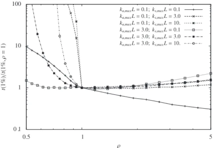
variance, increasing therefore the required number of realizations to reach a given accuracy. This is explored in
Figs. 5 and 6 that display the number of realizations
required to reach a 1% relative accuracy, as a function of ρ, that is to say as a function of the amount of negative null-collisions. Simulation results are given for ζ ¼ 1 and ζ ¼ 0:1 in order to evaluate whether the new algorithm
encounters more or less convergence difficulties when ^k is locally lower than the total extinction coefficient. We concentrate on the location x0¼ ½−L; 0; 0' as it was identi-fied as the most pathological condition: the starting point of all rays is right inside the region where ^kok (the negative null-collision region). Obviously the main trends of our algorithm are identical to those of[3]only observing that
%
we encounter more convergence difficulties when the negative null-collision region is optically thin in absorption and optically thick in scattering;%
when the medium is optically thin both in absorption and scattering, increasing the number of null-collisions decreases the 1%-accuracy computation-time, because the repeated computations of the absorption contribu-tions lead to a quasi-deterministic integration along the path, which reduces significantly the variance (more than it increases the computation-time), just as expected in standard energy partitioning approaches.4. Production of reference solutions for PRISSMA validation
The objective of the Monte Carlo algorithm proposed in
Section 2 is essentially to produce reference solutions
against which faster radiative transfer solvers can be validated. We here take the example of validating the PRISSMA solver that is implemented for representation of infrared radiative sources in AVBP (a parallel CFD code for reactive unsteady flow simulations on hybrid grids3). We
retain a configuration that was studied by Knikker et al.
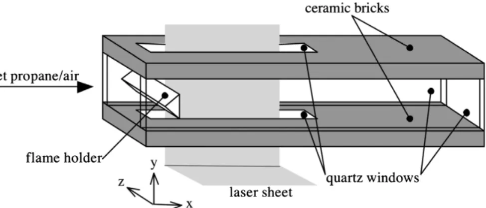
[19–21]. The dimensions of the chamber are the following
(seeFig. 7for axis conventions): 50 mm along the Y-axis,
80 mm along the Z-axis and 300 mm along the X-axis. A triangular flame hook is located on lateral sides, at a height of 25 mm. A air/propane mixture is injected from the left-hand side, and a V-shaped flame develops in the rectan-gular tube along the X-axis. Wall temperature is fixed to
Fig. 3. Time to reach a 1% standard deviation as a function of ζ, ka;maxL,
ks;maxLat x0¼ ½−L; 0; 0', for ε ¼ 0 and ^k ¼ ka;maxþ ks;max.
Fig. 4. Time to reach a 1% standard deviation as a function of ζ, ka;maxL,
ks;maxLat x0¼ ½−L; 0; 0', for ε ¼ 1 and ^k ¼ ka;maxþ ks;max.
Fig. 5. Time to reach a 1% standard deviation as a function of ρ, ka;maxL,
ks;maxLat x0¼ ½−L; 0; 0' for ε ¼ 1 and ζ ¼ 1.
Fig. 6. Time to reach a 1% standard deviation as a function of ρ, ka;maxL,
ks;maxLat x0¼ ½−L; 0; 0' for ε ¼ 1 and ζ ¼ 0:1.
300 K everywhere, except for outlet walls that have been set at 1900 K, the temperature of exhaust gases. As far as radiative properties are concerned, all boundaries are modeled as grey interfaces. The ceramic wall emissivity is set at ε ¼ 0:91. That of quartz windows is ε ¼ 0:87. The flame holder emissivity is ε ¼ 0:40, corresponding to a stainless steel lightly oxidized at 1000 K. The inlet, the outlet and the atmosphere are assumed to behave as black surfaces.
AVBP was run using a time averaged LES [22,23],
leading to the fields of temperature and species concen-trations displayed in Fig. 8. The radiative transfer solver embedded in AVBP, and therefore involved in the produc-tion of these fields, is PRISSMA[14]. It has been specifically designed for combustion applications. Based on a Discrete Ordinate Method[24], it is designed to reach a satisfactory compromise between accuracy and computational costs. The radiative budget is determined in the whole volume using a specific grid, coarser than the LES one. The associated strategy for the coupling with AVBP is detailed in[14]. The angular quadrature chosen here is an S4. The full spectrum model (FSK) is used for spectral integration using 15 quadrature points[23].
In order to meet the requirements of AVBP in terms of computation requirements, the spatial and angular discretiza-tions as well as the FSK spectral integration procedure were tuned at the extreme limits of their validity ranges, and it is therefore required that PRISSMA is validated against a refer-ence radiative transfer solver each time a new combustion
configuration is considered. This task is here achieved using the Monte Carlo algorithm ofSection 2, implemented within the EDStar development environment [10,13], using the Mcm3D library[25]. This implementation deals with three-dimension geometries using advanced computer-graphics tools. The input fields are the output of AVBP. Unlike in the benchmark simulations ofSection 3 where the input fields were analytic, the input fields are now provided using the LES grid of AVBP (4.74 million tetrahedrons) together with an interpolation procedure provided by the combustion specia-lists to reflect the spatial integration schemes involved in the fluid mechanics and chemistry solvers. As radiative transfer specialists, we therefore make no choice: we strictly accept what would be, ideally, the input fields that PRISSMA should reflect, in its coupling with AVBP, if no computation constraint was taken into account. Ideally, along the same line, our Monte Carlo simulations should use the best gaseous line-absorption properties available, i.e. the detailed line profiles provided by spectroscopic databases such as HITEMP[26]and CDSD[27]. However, at the present stage, only few attempts were reported in which such line-by-line Monte Carlo strate-gies were tested and none of them are compatible with our requirements in terms of three-dimension geometry and heterogeneity. As described in Section 2.3, our “reference” simulation makes therefore only use of a narrow band k-distribution strategy. The corresponding spectral data were produced using the SNB-ck approach of[28–31], separating CO2and H2O thanks a decorrelation assumption described at the end of Section 2.3. Three hundred sixty-seven spectral narrowbands are used, each of width Δν ¼ 25 cm−1, and the
Fig. 7. Representation of the dihedral combustion chamber.
Fig. 8. Visualization of the temperature field (K), CO2concentration field (molar fraction), H2O concentration field (molar fraction) and CO con-centration field (molar fraction) within the dihedral combustion chamber.
Fig. 9. Visualization of the radiative budget (W/m3) within the dihedral combustion chamber.
discrete-k sets are constructed in accordance with a Gauss– Legendre quadrature of order 7.
Altogether, in the validation exercise reported here, the objective was to validate PRISSMA in which
%
spatial integration relies on an adapted grid, coarser than the LES grid of AVBP, at the limits of the validity of spatial integration criteria (which will lead to unsmooth simulation results),%
angular discretization is reduced to a S4 quadrature,%
spectral integration is performed using only 15 FSK-quadrature points,and we validate it against a Monte Carlo solver that
%
uses the LES input fields,%
makes no approximation as far as angular integration is concerned,%
and uses a narrow-band discretization together with a k-distribution model for spectral integration.The main advantage of null-collisions was that the Monte Carlo solver could be designed completely independently of the LES grid structure. It can therefore be immediately used for validation of other configurations in which AVBP is run with another spatial-discretization strategy, or for validation of radiative solvers embedded in other combus-tion solvers (Fig. 9).
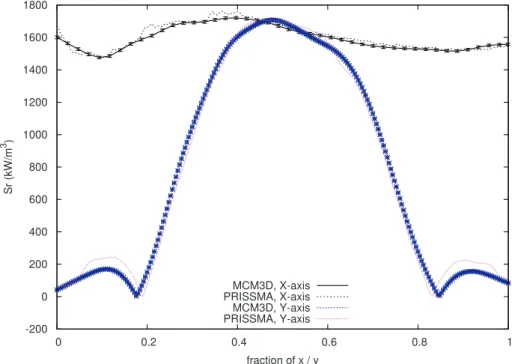
Typical results of this validation exercise are illustrated
in Fig. 10, where radiative budgets (W/m3) are presented
along the X-axis (y¼0, z¼0, x∈½0; 0:3' m) and along the Y-axis (x¼0.08, y∈½−0:025; 0:025 mÞ, z¼0). They reflect what would globally be interpreted as a good agreement in the combustion simulation context. PRISSMA and Mcm3D do not differ by more than a few percent in the regions where
radiative source terms are high. In the flame edges that are cold regions where the radiative source term is small, the results show significant discrepancies. In such zones the radiative species are more absorbing than emitting, and the accuracy of the solution is probably more sensitive to the DOM angular discretization. But such discrepancies have been shown to have little influence on the overall combustion simulation. In any case, provided that we assume that our narrow band model is sufficiently accu-rate, the Monte Carlo solution can be interpreted as the exact solution (within the statistical error bars) of the radiative transfer equation for the input fields that com-bustion specialists define as the complete continuous fields corresponding to the AVBP output. The question of inter-preting the discrepancies between PRISSMA and Mcm3D is therefore only a question of validating or invalidating the compromises made in the DOM simulation to meet AVBP's requirements in terms of computation times. Combustion specialists are then in the position of refining the PRISSMA grid, increasing the angular quadrature order, increasing the FSK quadrature order, as a function of the assumed sensitivity of their fluid mechanics/chemistry results to the radiative-transfer source-field.
Coming back to the validation tool itself, and thinking of the benchmark simulation results of Section 3, it is worth mentioning here that the computation time is highly dependent on the numerical optimization of the localization/interpolation procedure. All the null-collision algorithm needs, in order to deal with AVBP fields, is a function that takes the three geometrical coordinates as input and provides the local values of temperature, pres-sure and concentrations. This procedure needs to detect the tetrahedron to which the location belongs, and then apply an interpolation procedure compatible with AVBP's numerical assumptions (here a standard barycentric 3D
interpolation [35]). All CFD simulation environments
provide such functions, at least for post-treatment pur-poses. But the corresponding numerics can be extremely slow because post-treatments are not looped into iterative algorithms. In our Monte Carlo algorithm, we need to call this function at each collision event. Therefore the com-putation times are very sensitive to the numerics of the localization and interpolation procedure. Then the ques-tion becomes the following: as the Monte Carlo code is only used for validation purposes, one may use post-treatment tools without much concern (relying on paral-lelization to speed-up the Monte Carlo simulation), but if validation exercises are to be launched in a quite systema-tic manner, then localization/interpolation becomes an issue. Typically, in the above example, when using a localization/interpolation function extracted from post-treatment tools, the computation times needed to reach a 1% uncertainty were as high as 4 h on a single processor, whereas the same simulation (using the same interpola-tion funcinterpola-tion) was reduced to 40 s using standard acceleration-grids [35,36] to speed up the localization among the 4.74 millions tetrahedrons. In summary, deal-ing with three-dimension geometry and spectral integra-tion rises the computaintegra-tion times from several seconds, as
inSection 3, to several tens of seconds, but without caring
about the quality of the localization/interpolation proce-dure, a jump is made up to several hours.
Note finally that CFD simulation environments may provide optimized localization/interpolation tools if they address the question of the flow transporting solid or liquid particles, because for different reasons they have the same need to establish the correspondence between the location of a particle and the characteristics of the flow it encounters.
5. Conclusion
Validating the radiative transfer solvers embedded in combustion simulation codes is an important issue. These solvers need to be very fast, which leads the developers to play, as finely as possible, with the limits of validity of the retained numerical techniques. This is particularly true as far as absorption line-spectra representation and phase-space discretization are concerned. It is therefore essential that the corresponding numerical parameters be adjusted to each new combustion configuration, or at least that their effect be controlled each time a new configura-tion is addressed. From this point of view, the fact that Monte Carlo solvers deal now easily with complex geo-metries is a key element. We essentially benefit of the advances of the computer graphics community: path-tracking algorithms are now sufficiently efficient and easy-to-handle to meet our needs. Starting from the geometric CAD file of a new combustion chamber and sampling optical paths in the corresponding complex geometry is now ready-for-use. For Monte Carlo codes to be implemented that could easily deal with all the diver-sity of combustion codes and the diverdiver-sity of combustion configurations, the missing point is therefore only the representation of the temperature, pressure and concen-tration fields. In each new context, these fields are pro-vided under different mathematical forms, with different
formats, and it is nearly required to design a new Monte Carlo code for each new combustion-code validation exercise.
The algorithm presented in the present paper was meant as a contribution to such today's researches. The initial idea was to explore a technical solution used in neutron and electron-transport physics to deal with het-erogeneous fields: the introduction of null-collisions, that change nothing to the transport of particles, but that can be tuned so that the total extinction coefficient becomes homogeneous (or easy to handle). This idea was addressed theoretically in [3] and we here explored its practical meaning in the combustion-simulation context. We reach the conclusion that null-collision Monte Carlo algorithms are well suited. Combustion specialists wishing to validate their radiative solver have nothing more to provide than a function interpolating their grid point simulation results to give the temperature, pressure and concentrations at any given location. This commonly implies a localization procedure (typically to determine what tetrahedron the considered location belongs to) and an interpolation procedure in accordance with the spatial schemes used in their fluid mechanics and chemistry codes. This last point is essential in order to make sure that the continuous input fields provided to the Monte Carlo solver are correct representations of the numerical assumptions made within the combustion code. Usually, such localiza-tion and interpolalocaliza-tion routines are available, at least for the post-treatment of combustion simulation results. They can however be extremely slow, which can be a source of difficulty if the number of required validation exercises is high. We saw, in the last section, that the Monte Carlo computation times can rise from less than a minute to a few hours when switching to a very slow localization procedure, but these computation times were given without the use of any parallel hardware. Few hours may then sound very much acceptable for only a validation exercise. Otherwise, as we illustrated it, some additional efforts can be made to build a better optimized localization procedure, considering that it is meant to be used for each of the very numerous colli sion locations sampled in the Monte Carlo algorithm. This simply implies using acceleration grids but will only be required if validation exercises are frequently repeated.
By comparison with[3], we upgraded the algorithm in order to follow the path continuously and only exit after absorption when an extinction criterion is reached. This upgrade, that involves a quite limited number of algorith-mic changes, is particularly meaningful in the combustion context because combustion chambers are commonly optically quite thin at most frequencies, and path-continuation reduces significantly the required computa-tion times, for a given accuracy, in the optically thin limit. In thicker conditions, our new proposition may be worse than the initial one, but then the computation-time increase is only limited. So, when we are faster, the gain can be very significant, and when we are slower, the loss is limited. We therefore conclude that our new algorithm is worth being preferred systematically to that of [3], except in contexts where the computational
constraints are high and justify that ζ is adapted to the values of both the scattering and absorption optical thicknesses.
Finally, as in[3], the algorithm is designed to allow the occurrence of negative null-collisions. Of course this is at the price of an increased variance. But pathological beha-viors are only encountered when the region of negative null-collisions is optically thick with a high single scatter-ing albedo. Again, optically thick scatterscatter-ing is quite rare among combustion configurations and the ^k field can therefore be chosen without caring too much about the risk that, because of the non-linear dependence of absorp-tion coefficients with temperature, ^k is not a rigorous upper bound to k at all locations.
Acknowledgments
The research presented in this paper was conducted with the support of the STRASS project funded by the Fédération Recherche Aéronautique et Espace (FRAE). V.E. also acknowledges support from the European Research Council (Starting Grant 209622: E3ARTHs).
References
[1]Zhang J, Gicquel O, Veynante D, Taine J. Monte Carlo method of radiative transfer applied to a turbulent flame modeling with LES. Comptes rendus. Mécanique. ISSN: 1631-0721 INCA (Initiative on Advanced Combustion) Workshop No. 2, Rouen , France (23/10/ 2008), vol. 337, no. 6–7; 2009. p. 539–49.
[2]Zhang J. Radiation Monte Carlo approach dedicated to the coupling with LES reactive simulation. PhD thesis, EM2C; 2011.
[3]Galtier M, et al. Integral formulation of null-collision Monte Carlo algorithms. J Quant Spectrosc Radiat Transfer, in press 〈http://dx.doi. org/10.1016/j.jqsrt.2013.04.001〉.
[4] Farmer JT, Howell JR. Comparison of Monte Carlo strategies for radiative transfer in participating media. Adv Heat Transfer 1998;31: 333–429.
[5]Modest M. Radiative heat transfer. 3rd ed. Academic Press; 2013. ISBN-10: 0123869447, ISBN-13: 978-0123869449.
[6] De Lataillade A, Dufresne JL, El Hafi M, Eymet V, Fournier R. A net exchange Monte-Carlo approach to radiation in optically thick systems. J Quant Spectrosc Radiat Transfer 2002;74:563–84. [7] Eymet V, Dufresne JL, Fournier R, Blanco S. A boundary-based net
exchange Monte-Carlo Method for absorbing and scattering thick medium. J Quant Spectrosc Radiat Transfer 2005;95:27–46. [8] Eymet V, Dufresne JL, Ricchiazzi P, Fournier R, Blanco S. Longwave
radiative analysis of cloudy scattering atmospheres using a net exchange formulation. Atmos Res 2004;72:238–61.
[9]Eymet V, Fournier R, Dufresne J-L, Lebonnois S, Hourdin F, Bullock MA. Net-exchange parameterization of thermal infrared radiative transfer in Venus' atmosphere. J Geophys Res 114:2009;E11008. DOI: http://dx.doi.org/10.1029/2008JE003276.
[10] Delatorre J, Bézian JJ, Blanco S, Caliot C, Cornet JF, Dauchet J, et al. Monte-Carlo advances and concentrated solar applications. Solar Energy, in press 〈http://dx.doi.org/10.1016/j.solener.2013.02.035〉. [11] Rehfeld N, Stute S, Soret M, Apostolakis J, Buvat I. Optimization of
photon tracking in gate. In: Nuclear science symposium conference record, NSS'08. IEEE; 2008. p. 4013–5.
[12] Badal A, Badano A. Monte Carlo simulation of x-ray imaging using a graphics processing unit. In: Nuclear science symposium conference record (NSS/MIC), 2009. IEEE; 2009. p. 4081–4.
[13] Edstar (starwest development environment) 〈http://www.starwest. ups-tlse.fr/edstar/edstar.html〉, including the codes of the four appli-cation examples at 〈 http://www.starwest.ups-tlse.fr/monte-carlo-concentrated-solar-examples/〉.
[14] Poitou D, Amaya J, El Hafi M, Cuenot B. Analysis of the interaction between turbulent combustion and thermal radiation using
unsteady coupled LES/DOM simulations. Combust Flame 2011;159 (4):1605–18.
[15] Shamsundar N, Sparrow EM, Heinisch RP. Monte Carlo radiation solutions—effect of energy partitioning and number of rays. Int J Heat Mass Transfer 1973;16:690–4.
[16] Wang A, Modest MF. An adaptive emission model for Monte Carlo simulations in highly inhomogeneous media represented by sto-chastic particle fields. J Quant Spectrosc Radiat Transfer 2006;104: 288–96.
[17] André F, Vaillon R. Generalization of the k-moment method using the maximum entropy principle. Application to the NBKM and full spectrum SLMB gas radiation models. J Quant Spectrosc Radiat Transfer 2012;113:1508–20.
[18] Dauchet J, Blanco S, Cornet JF, EL Hafi M, Eymet V, Fournier R. The practice of recent radiative transfer Monte Carlo Advances and its contribution to the field of microorganisms cultivation in photo-bioreactors. J Quant Spectrosc Radiat Transfer, in press 〈http://dx.doi. org/10.1016/j.jqsrt.2012.07.004〉.
[19] Knikker R, Veynante D, Rolon JC, Meneveau C. Planar laser-induced fluorescence in a turbulent premixed flame to analyze large eddy simulation model. In: Proceedings of the 10th international sympo-sium on applications of laser techniques to fluid mechanics., 2000. [20] Knikker R, Veynante D, Meneveau C. A priory testing of a similarity
model for large eddy simulations of turbulent premixed combus-tion. Proc Combust Inst 2002;29(2):2105–11.
[21]Nottin C, Knikker R, Boger M, Veynante D. Large eddy simulations of an acoustically excited turbulent premixed flame. In: Symposium (international) on combustion, vol. 28(1); 2000. p. 67–73.
[22] Poitou D. Modélisation du rayonnement dans la simulation aux grandes échelles de la combustion turbulente. PhD thesis, Thèse de doctorat, Institut National Polytechnique de Toulouse; 2009.
[23] Poitou D, El Hafi M, Cuenot B. Analysis of radiation modeling for turbulent combustion: development of a methodology to couple turbulent combustion and radiative heat transfer in LES. J Heat Transfer 2011;133:062701–10.
[24] Joseph D, El Hafi M, Fournier R, Cuenot B. Comparison of three spatial differencing schemes in Discrete Ordinates Method using three-dimensional unstructured meshes. Int J Thermal Sci 2005;44 (9):851–64.
[25] 〈http://www.starwest.ups-tlse.fr/edstar/mcm3d.html〉.
[26] Rothman LS, Gordon LE, Barber RJ, Dothe H, Gamache RR, Goldman A, et al. HITEMP, the high-temperature molecular spectroscopic database. J Quant Spectrosc Radiat Transfer 2010;111(15):2139–50. [27] Tashkun SA, Perevalov VI. CDSD-4000, resolution,
high-temperature carbon dioxide spectroscopic databank. J Quant Spec-trosc Radiat Transfer 2011;112(9):1403–10.
[28] Soufiani A, Taine J. High temperature gas radiative property para-meters of statistical narrow band model for H2O, CO2and CO and correlated-k model for H2O and CO2. Int J Heat Mass Transfer 1997;40(4):987–91.
[29] Liu F, Smallwood GJ, Gulder OL. Application of the statistical narrow-band correlated-k method to low-resolution spectral inten-sity and radiative heat transfer calculations—effects of the quad-rature scheme. Int J Heat Mass Transfer 2000;43:3119–25. [30] Liu F, Smallwood GJ, Gulder OL. Application of the statistical
narrow-band correlated-k method to non-grey gas radiation in CO2–H2O mixtures: approximate treatments of overlapping bands. J Quant Spectrosc Radiat Transfer 2001;68:401–17.
[31] Joseph D, Perez P, El Hafi M, Cuenot B. Discrete ordinates and Monte Carlo methods for radiative transfer simulation applied to computa-tional fluid dynamics combustion modeling. J Heat Transfer 2009;131:052701.
[32] Wang A, Modest MF. Spectral Monte Carlo models for nongray radiation analyses in inhomogeneous participating media. J Heat Mass Transfer 2009;50:3877–89.
[33] Fomin A. Monte Carlo algorithm for line-by-line calculations of thermal radiation in multiple scattering layered atmospheres. J Quant Spectrosc Radiat Transfer 2006;98:107–15.
[34] Taine J, Soufiani A. Gas IR radiative properties: from spectroscopic data to approximate models. Adv Heat Transfer 1999;33:295–414. [35] Pharr M, Humphreys G. Physically based rendering: from theory to
implementation. Elsevier; 2004.
[36] Fujimoto A, Tanaka T, Iwata K. Arts: acceleration ray-tracing system. IEEE Comput Graph Appl 1986;6(April (4)):16–26.
[37] Siegel R, Howell JR. Thermal radiation heat transfer. 5th ed. CRC Press; 2010. ISBN-10: 1439805334, ISBN-13: 978-1439805336.
![Fig. 1. Description of the proposed algorithm. It follows an energy-partitioning strategy until the extinction term ξ is less than a fixed criterion ζ in which case it switches to the algorithm introduced in [3].](https://thumb-eu.123doks.com/thumbv2/123doknet/12425705.334144/5.892.76.838.106.647/description-proposed-algorithm-partitioning-extinction-criterion-algorithm-introduced.webp)
![Fig. 2. Considered system: a cube of side 2L, whose center is the Cartesian coordinate system origin (figure taken from [3]).](https://thumb-eu.123doks.com/thumbv2/123doknet/12425705.334144/8.892.181.702.753.1135/fig-considered-center-cartesian-coordinate-origin-figure-taken.webp)