ÉCOLE DE TECHNOLOGIE SUPÉRIEURE UNIVERSITÉ DU QUÉBEC
THESIS PRESENTED TO
ÉCOLE DE TECHNOLOGIE SUPÉRIEURE
IN PARTIAL FULFILLMENT OF THE REQUIREMENTS FOR THE DEGREE OF DOCTOR OF PHILOSOPHY
Ph.D
BY
MARTENS, Walter
MULTIPATH PROPAGATION MODELS FOR NEAR LINE-OF-SIGHT CONDITIONS
MONTRÉAL, DECEMBER 8, 2009 © Copyright 2009 reserved by Walter Martens
THIS THESIS HAS BEEN EVALUATED BY THE FOLLOWING BOARD OF EXAMINERS
Mr. Francois Gagnon, Thesis Supervisor
Département genie electrique à l’École de technologie supérieure
Mr. Naim Batani, Thesis Co-director
Département de génie électrique à l’École de technologie supérieure
Mr. Eric David President of the Board of Examiners
Département de génie mécanique à l’École de technologie supérieure
Mr. Christian Gargour, Member of the Jury
Département de génie électrique à l’École de technologie supérieure
Mr. Sofiene Affes, External Examiner
INRS Énergie, Matériaux et Télécommunication
THIS THESIS WAS PRESENTED AND DEFENDED BEFORE A BOARD OF EXAMINERS AND PUBLIC
NOVEMBER 11, 2009
ACKNOWLEDGEMENTS
The author wishes to thank Prof. François Gagnon and Prof. Naim Batani, co-directors of this thesis. Dr. Gagnon provided insightful advice and many fruitful discussions about this work.
The author also wishes to thank Ultra Electronics Tactical Communications Systems of Montreal, Quebec, Canada for their support of this work, for the use of the equipment to perform the measurements and permission to use the results. The author is grateful to his colleagues at Ultra Electronics, Mr. Michael Darsigny, Mr. Maurice Chalifoux and Mr. David Trudeau for their assistance in organizing and carrying out the experiments whose results are described in this thesis.
Finally, the author would like to thank his wife, Dr. Chen Liu, for her encouragement and support of this project.
MULTIPATH PROPAGATION MODELS FOR NEAR LINE-OF-SIGHT CONDITIONS
MARTENS, Walter RÉSUMÉ
Cette thèse porte sur le comportement d’un canal à propagation par trajets multiples dont le lien est en visibilité directe ou dont les pertes additionnelles dues aux obstacles sont très faibles. Ce type de canal existe dans les banlieues ou les régions presque rurales. L’objectif de ce projet de recherche est de caractériser le comportement à large bande de ce type de canal. La thèse comporte cinq parties majeures : la problématique et revue de la littérature, une analyse théorique, des mesures expérimentales pour valider l’analyse, des applications aux canaux pratiques et une étude des effets d’un tel canal sur les signaux typiques.
Les amplitudes et l’étalement du délai pour un modèle de propagation à trajets multiples réaliste de cet environnement sont étudiés. Ceci se base sur une analyse théorique de la réflexion des surfaces plates finies qui représentent des murs de bâtiments. À partir de cette analyse, un modèle à large bande est proposé. La partie suivante de la thèse présente les résultats des mesures expérimentales pour les canaux de propagation à trajets multiples dans les banlieues et les régions presque rurales. Dans ces conditions, les liens sont en visibilité directe ou encore, les pertes additionnelles dues aux obstacles sont très faibles. Les résultats confirment l’analyse théorique. Selon les régions mises à l’essai, on observe un canal soit très bon ou encore très mauvais. Un canal mauvais se trouve généralement près d’un bâtiment où il existe une seule réflexion dominante dont le délai relatif est de moins d’une microseconde. Cette réflexion cause des évanouissements est des distorsions sévères du signal qui rend le canal souvent inutilisable. L’aire de la région pour laquelle le canal est mauvais dépend de la largeur du bâtiment.
Après les résultats expérimentaux, la thèse décrit quelques applications du modèle à large bande et analyse les effets du modèle proposé sur les signaux typiques de communication comme la modulation en quadrature de phase, QPSK, la modulation par étalement du spectre en séquence directe et la modulation utilisant des sous-porteuse orthogonales, OFDM. Pour le signal QPSK, les effets d’une seule réflexion dominante sur les circuits pour la récupération de l’horloge et de la porteuse d’un démodulateur sont étudiés. Une méthode est aussi présentée pour déterminer les endroits dans lesquels les liens seront sévèrement dégradés.
Mots clés: Communication numérique, propagation, trajets multiples, réflexion, synchronisation
MULTIPATH PROPAGATION MODELS FOR NEAR LINE-OF-SIGHT CONDITIONS
MARTENS, Walter ABSTRACT
This thesis analyzes the behaviour of a multipath channel for suburban and semi-rural areas in which line of sight (LOS) or near LOS exists between the transmitter and receiver. The objective is to characterize the broadband channel for such areas. The thesis is divided into five major parts: a background and literature survey, a theoretical analysis, experimental measurements which validate the analysis, applications to practical communication channels and a study of the effects of such a channel on typical signal waveforms.
The amplitudes and delay spread of a multipath model for such an environment are studied, based on a theoretical analysis of scattering from finite flat surfaces which model building walls. A broadband channel model is proposed based on the analysis. The next part of the thesis presents experimental measurements on multipath communication channels in suburban and semi-rural areas, which have LOS or near LOS propagation. The results validate the theoretical analysis. It is found that the channel is either good or very bad. The latter usually occurs close to buildings where a single dominant reflection with a relative delay of less than a microsecond produces a periodic severe fading and distortion of the signal, often making a link unusable. The area for which the channel is bad depends on the size of the building.
The thesis then considers applications of the broadband channel model and studies the effects of the proposed channel model on typical communication waveforms such as QPSK, direct sequence spread spectrum and OFDM. For the QPSK waveform, the effects of a single dominant reflection on the timing and carrier recovery of a coherent demodulator are studied. A methodology is also outlined for determining which locations in a defined area will show the behaviour associated with a bad channel.
TABLE OF CONTENTS
Page
INTRODUCTION ... 1
CHAPTER 1 BACKGROUND AND LITERATURE SURVEY ... 4
CHAPTER 2 THEORY ... 11
2.1 General ... 11
2.2 Theoretical analysis of reflection from a flat wall ... 13
2.3 Reflection from other surfaces ... 32
2.4 Summary and evaluation of analysis results ... 35
CHAPTER 3 EXPERIMENTAL RESULTS ... 38
3.1 General ... 38
3.2 Experimental results... 39
3.2.1 Measurement methods ... 39
3.2.2 Results ... 42
3.2.3 Summary and analysis of experimental results ... 80
CHAPTER 4 APPLICATIONS ... 81
4.1 Propagation models for practical channels ... 81
4.2 Estimation of link availability ... 82
4.3 Example of outage area prediction ... 87
CHAPTER 5 EFFECTS OF SINGLE DOMINANT REFLECTION ON SIGNAL MODULATION ... 96
5.1 General ... 96
5.2 Mathematical models of modulated signals ... 98
5.3 Delay and doppler effects ... 99
5.4 Effect of reflections on modulated signals ... 100
5.5 Effects of single dominant reflection on signal spectrum ... 104
5.6.1 Aspects of synchronization ... 105
5.6.2 Steady state timing and carrier recovery phase errors due to single reflection………109
5.7 Direct sequence spread spectrum systems ... 111
5.8 OFDM systems ... 113
5.9 Performance of other receivers ... 116
CONCLUSIONS... 120
ANNEX QPSK TIMING AND CARRIER RECOVERY SIMULATIONS ... 123
LIST OF FIGURES
Page
Figure 2.1 Propagation model. ... 14
Figure 2.2 Vertical electric field magnitude, 10m × 10 m wall. ... 22
Figure 2.3 Vertical electric field magnitude, 10 m × 20 m wall. ... 23
Figure 2.4 Vertical electric field magnitude, 20m × 10 m wall. ... 24
Figure 2.5 Planar X-Y electric field distribution, 10m × 10m wall. X scale in m, wall extends from x = 6 to 16; Y scale in m from top, wall located at y = -3. ... 25
Figure 2.6 Vertical electric field magnitude, 10 m × 10 m wall, ground reflection. Red: direct field, Black: reflected field. ... 30
Figure 2.7 Vertical electric field magnitude, 10 m × 20 m wall, ground reflection. Red: direct field, Black: reflected field. ... 31
Figure 2.8 Vertical electric field magnitude, 20 m × 10 m wall, ground reflection. Red: direct field, Black: reflected field. ... 32
Figure 3.1 Experimental link configuration. ... 40
Figure 3.2 QPSK receiver. ... 41
Figure 3.3 Binary FM receiver. ... 41
Figure 3.4 Distribution of error rates, suburban and rural links. ... 43
Figure 3.5 Mobile close to a building. ... 44
Figure 3.6 RF spectrum (18 February 2005). ... 45
Figure 3.7 RF spectrum (18 February 2005). ... 46
Figure 3.8 IF spectrum (18 February 2005). ... 47
Figure 3.9 IF spectrum (18 February 2005). ... 48
Figure 3.10 IF spectrum (18 February 2005). ... 49
Figure 3.12 Spectrum analysis (a & b). ... 53
Figure 3.13 Spectrum analysis (a & b). ... 54
Figure 3.14 Spectrum analysis (a & b). ... 55
Figure 3.15 Spectrum analysis (a & b). ... 56
Figure 3.16 RF level variation with time, slow random variations (18 February 2005). ... 59
Figure 3.17 RF level variation with time, random variations (18 February 2005). ... 60
Figure 3.18 RF level variation with time, small single reflection (18 February 2005). ... 61
Figure 3.19 RF level variation with time, small single reflection (18 February 2005). ... 62
Figure 3.20 IF level variation with time (18 February 2005). ... 63
Figure 3.21 IF level variation with time (18 February 2005). ... 64
Figure 3.22 IF level variation with time (18 February 2005). ... 65
Figure 3.23 IF level variation with time (18 February 2005). ... 66
Figure 3.24 IF level variation with time (18 February 2005). ... 67
Figure 3.25 IF level variation with time (18 February 2005). ... 68
Figure 3.26 IF level variation with time (18 February 2005). ... 69
Figure 3.27 Transmitted pulses (reference) (23 December 2004). ... 71
Figure 3.28 Transmitted pulse spectrum (23 December 2004). ... 72
Figure 3.29 Received pulse (23 December 2004). ... 73
Figure 3.30 Received pulse (23 December 2004). ... 74
Figure 3.31 Received pulse (23 December 2004). ... 75
Figure 3.32 Received pulse (23 December 2004). ... 76
Figure 3.33 Received pulse (23 December 2004). ... 77
Figure 3.34 Received pulse (23 December 2004). ... 78
Figure 4.1 Reflection delay geometry. ... 84
Figure 4.2 Outage area estimation. ... 86
Figure 4.3 Test route of the mobile (© Google 2009). ... 88
Figure 4.4 Magnified mobile route 1 (© Google 2009). ... 90
Figure 4.5 Magnified mobile route 2 (© Google 2009). ... 91
Figure 4.6 Magnified mobile route 3 (© Google 2009). ... 92
Figure 4.7 Magnified mobile route 4 (© Google 2009). ... 93
Figure 4.8 Magnified mobile route 5 (© Google 2009). ... 94
Figure 5.1 Standard receiver model. ... 102
Figure 5.2 Typical timing recovery function for QPSK. ... 106
Figure 5.3 QPSK constellation. ... 108
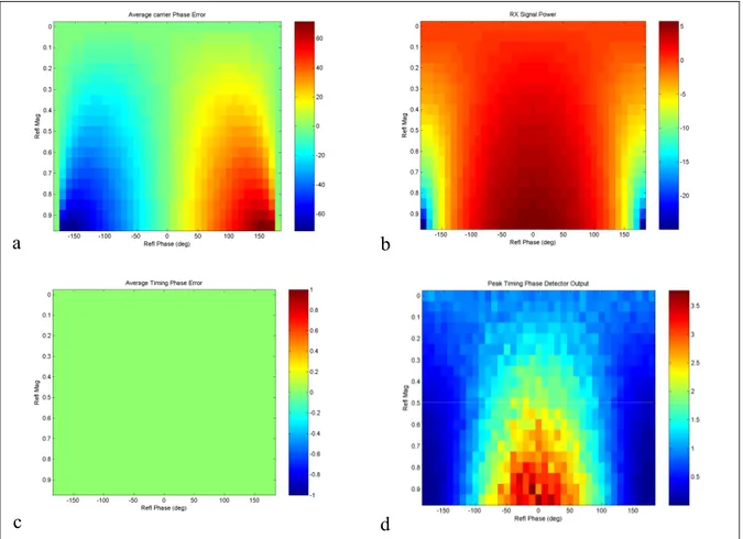
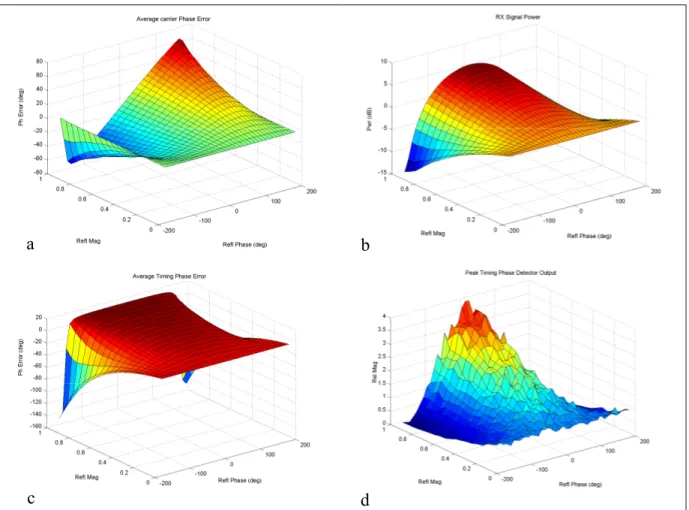
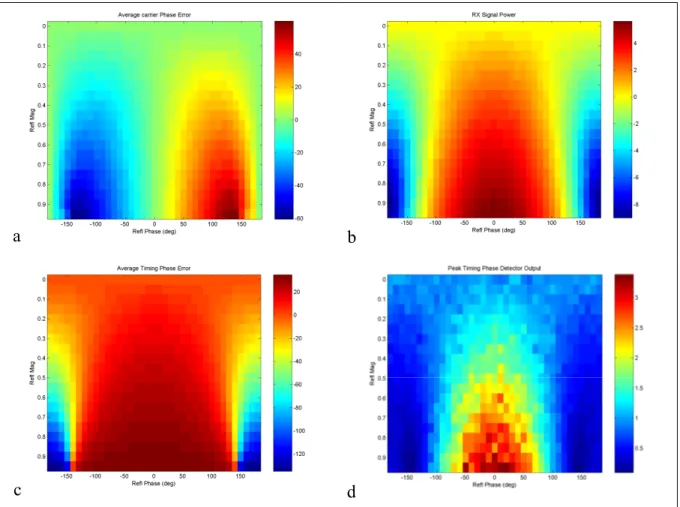
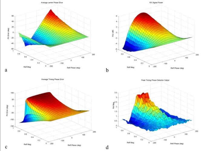
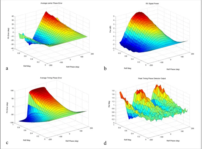
Figure A.1 Delay 0.0 symbols. a) average carrier phase error; b) received signal power; c) average timing phase error; d) peak timing phase detector output. ... 123
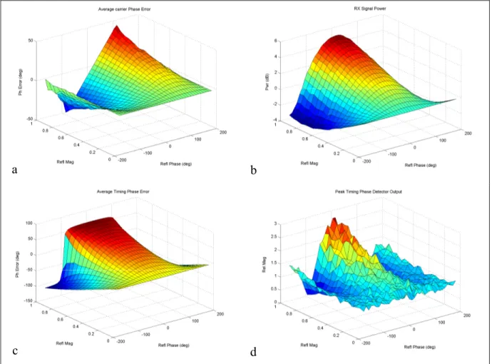
Figure A.2 Delay 0.0 symbols. a) average carrier phase error; b) received signal power; c) average timing phase error; d) peak timing phase detector output. ... 124
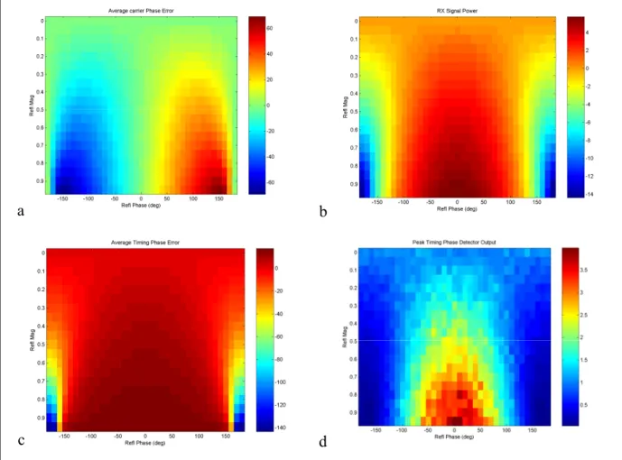
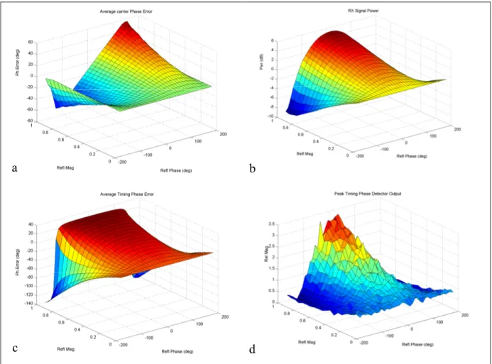
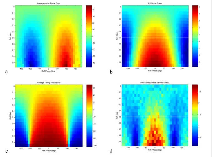
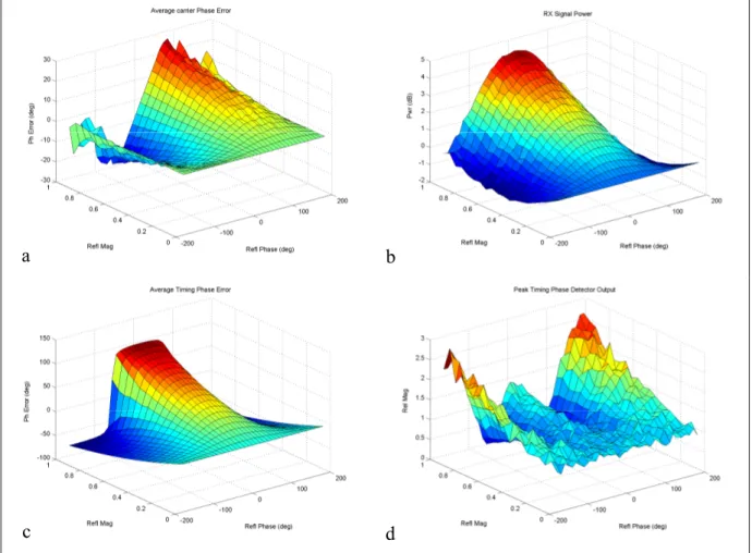
Figure A.3 Delay 0.1 symbols. a) average carrier phase error; b) received signal power; c) average timing phase error; d) peak timing phase detector output. ... 125
Figure A.4 Delay 0.1 symbols. a) average carrier phase error; b) received signal power; c) average timing phase error; d) peak timing phase detector output. ... 126
Figure A.5 Delay 0.2 symbols. a) average carrier phase error; b) received signal power; c) average timing phase error; d) peak timing phase detector output. ... 127
Figure A.6 Delay 0.2 symbols. a) average carrier phase error; b) received signal power; c) average timing phase error; d) peak timing phase detector output. ... 128
Figure A.7 Delay 0.3 symbols. a) average carrier phase error; b) received signal power; c) average timing phase error; d) peak timing phase detector output. ... 129 Figure A.8 Delay 0.3 symbols. a) average carrier phase error; b) received signal
power; c) average timing phase error; d) peak timing phase detector output. ... 130 Figure A.9 Delay 0.4 symbols. a) average carrier phase error; b) received signal
power; c) average timing phase error; d) peak timing phase detector output. ... 131 Figure A.10 Delay 0.4 symbols. a) average carrier phase error; b) received signal
power; c) average timing phase error; d) peak timing phase detector output. ... 132 Figure A.11 Delay 0.5 symbols. a) average carrier phase error; b) received signal
power; c) average timing phase error; d) peak timing phase detector output. ... 133 Figure A.12 Delay 0.5 symbols. a) average carrier phase error; b) received signal
power; c) average timing phase error; d) peak timing phase detector output. ... 134 Figure A.13 Delay 0.6 symbols. a) average carrier phase error; b) received signal
power; c) average timing phase error; d) peak timing phase detector output. ... 135 Figure A.14 Delay 0.6 symbols. a) average carrier phase error; b) received signal
power; c) average timing phase error; d) peak timing phase detector output. ... 136 Figure A.15 Delay 0.7 symbols. a) average carrier phase error; b) received signal
power; c) average timing phase error; d) peak timing phase detector output. ... 137 Figure A.16 Delay 0.7 symbols. a) average carrier phase error; b) received signal
power; c) average timing phase error; d) peak timing phase detector output. ... 138 Figure A.17 Delay 0.8 symbols. a) average carrier phase error; b) received signal
power; c) average timing phase error; d) peak timing phase detector output. ... 139 Figure A.18 Delay 0.8 symbols. a) average carrier phase error; b) received signal
power; c) average timing phase error; d) peak timing phase detector output. ... 140
Figure A.19 Delay 0.9 symbols. a) average carrier phase error; b) received signal power; c) average timing phase error; d) peak timing phase detector output. ... 141 Figure A. 20 Delay 0.9 symbols. a) average carrier phase error; b) received signal
power; c) average timing phase error; d) peak timing phase detector output. ... 142 Figure A.21 Delay 1.0 symbols. a) average carrier phase error; b) received signal
power; c) average timing phase error; d) peak timing phase detector output. ... 143 Figure A.22 Delay 1.0 symbols. a) average carrier phase error; b) received signal
power; c) average timing phase error; d) peak timing phase detector output. ... 144 Figure A.23 Delay 1.1 symbols. a) average carrier phase error; b) received signal
power; c) average timing phase error; d) peak timing phase detector output. ... 145 Figure A.24 Delay 1.1 symbols. a) average carrier phase error; b) received signal
power; c) average timing phase error; d) peak timing phase detector output. ... 146 Figure A.25 Delay 1.2 symbols. a) average carrier phase error; b) received signal
power; c) average timing phase error; d) peak timing phase detector output. ... 147 Figure A.26 Delay 1.2 symbols. a) average carrier phase error; b) received signal
power; c) average timing phase error; d) peak timing phase detector output. ... 148 Figure A.27 Delay 1.3 symbols. a) average carrier phase error; b) received signal
power; c) average timing phase error; d) peak timing phase detector output. ... 149 Figure A.28 Delay 1.3 symbols. a) average carrier phase error; b) received signal
power; c) average timing phase error; d) peak timing phase detector output. ... 150 Figure A.29 Delay 1.4 symbols. a) average carrier phase error; b) received signal
power; c) average timing phase error; d) peak timing phase detector output. ... 151 Figure A.30 Delay 1.4 symbols. a) average carrier phase error; b) received signal
power; c) average timing phase error; d) peak timing phase detector output. ... 152
Figure A.31 Delay 1.5 symbols. a) average carrier phase error; b) received signal power; c) average timing phase error; d) peak timing phase detector output. ... 153 Figure A.32 Delay 1.5 symbols. a) average carrier phase error; b) received signal
power; c) average timing phase error; d) peak timing phase detector output. ... 154 Figure A.33 Delay 1.6 symbols. a) average carrier phase error; b) received signal
power; c) average timing phase error; d) peak timing phase detector output. ... 155 Figure A.34 Delay 1.6 symbols. a) average carrier phase error; b) received signal
power; c) average timing phase error; d) peak timing phase detector output. ... 156 Figure A.35 Delay 1.7 symbols. a) average carrier phase error; b) received signal
power; c) average timing phase error; d) peak timing phase detector output. ... 157 Figure A.36 Delay 1.7 symbols. a) average carrier phase error; b) received signal
power; c) average timing phase error; d) peak timing phase detector output. ... 158 Figure A.37 Delay 1.8 symbols. a) average carrier phase error; b) received signal
power; c) average timing phase error; d) peak timing phase detector output. ... 159 Figure A.38 Delay 1.8 symbols. a) average carrier phase error; b) received signal
power; c) average timing phase error; d) peak timing phase detector output. ... 160 Figure A.39 Delay 1.9 symbols. a) average carrier phase error; b) received signal
power; c) average timing phase error; d) peak timing phase detector output. ... 161 Figure A.40 Delay 1.9 symbols. a) average carrier phase error; b) received signal
power; c) average timing phase error; d) peak timing phase detector output. ... 162 Figure A.41 Delay 2.0 symbols. a) average carrier phase error; b) received signal
power; c) average timing phase error; d) peak timing phase detector output. ... 163 Figure A.42 Delay 2.0 symbols. a) average carrier phase error; b) received signal
power; c) average timing phase error; d) peak timing phase detector output. ... 164
LIST OF ABBREVIATIONS AND ACRONYMS AGC BPSK CDMA CW dB DC DS DSSS FFT GO IDFT IF Km Km/hr LAN LOS Mb/s MHz MLSD μs OFDM PO QAM QPSK RAKE RF RCS SUI
Automatic gain control Binary phase shift keying Code division multiple access Continuous wave
Decibel
Direct current (refers to zero frequency) Direct sequence
Direct sequence spread spectrum Fast Fourier transform
Geometric optics
Inverse discrete Fourier transform Intermediate frequency
Kilometre
Kilometres per hour Local area network Line of sight
Megabits per second Megahertz
Maximum likelihood sequence detector Microsecond
Orthogonal frequency division multiplexing Physical optics
Quadrature amplitude modulation Quaternary phase shift keying
Type of receiver for a direct sequence spread spectrum signal Radio frequency
Radar cross section
UTD UWB WiMAX
Unified theory of diffraction Ultra wideband
LIST OF SYMBOLS H W a b r ρg , ρg1, ρg2 ρw E Ei Es ESZ S λ j d d0 σR PD0 PDi Z0 A Ht Hi J x, y, z I l R θ
height of a reflecting wall width of a reflecting wall height of base station antenna height of mobile antenna
distance from base station to mobile ground plane reflection coefficients wall reflection coefficient
electric field
incident electric field scattered electric field
scattered electric field in z direction scattering matrix
wavelength square root of -1
distance from scatterer or reflector to receiver near zone distance
radar cross section scattered power density incident power density
wave impedance of free space area
tangential magnetic field incident magnetic field current density
rectangular coordinate system current
length of current element distance from radiating element
Δx, Δy, Δz ac C, S P G R1, R2 R3, R4 R5, R6 σ η ρg1, ρg2 , ρg3 ρw ω ξ, ξr θ1 θ5 θ6 h w ρ r1, r2 rS1, rS2 AS σS γ V V1 f f0 U increments of x, y, z radius of circular flat plate Fresnel integrals
transmitted power base station antenna gain
distances from base station and base station image to mobile respectively distances from base station and its image to a wall element
distances of a wall element and its image respectively to the mobile antenna ground conductivity
electrical parameter of round reflection coefficients of ground reflection coefficient of ground radian frequency
permittivity and relative permittivity respectively
angle from the vertical of the vector from the base station image to the mobile angle from vertical to vector from base station image to mobile unit
angle from vertical to vector from wall image to mobile unit height of a rectangular surface
width of a rectangular surface general reflection coefficient
principal radii of curvature of reflected wavefront principal radii of curvature of reflective surface
attenuation of reflected wave due to surface roughness rms surface roughness
grazing angle
lowpass power spectrum complete power spectrum frequency
carrier frequency
U1 Up Uq τ xb yb Uyb t ti i t0, t1, t2 ai a0, a1, a2 β φi b Rb Rm Rbm θr ΔR c Rs p q s z apn aqn n autocorrelation function inphase part of U1 quadrature part of U1 delay amplitude modulation autocorrelation function of yb total signal time delay of ith component index variable delay of components 0, 1, 2 amplitude of ith component amplitude of components 0, 1, 2 phase modulation
phase shift of ith component relative amplitude of reflection
distance of base station from reflecting wall distance from reflecting wall to mobile distance from base station to mobile reflection angle
difference in distance between direct and reflected components speed of light symbol rate in-phase component quadrature component signal waveform analytic signal
amplitude of nth symbol in in-phase part amplitude of nth symbol in quadrature part index variable
T u z1 rtr v θr fd rr arn fdn θ0n Δτn Δfn Δθn Rr P Q F α0 α1 Pd Kd Rc symbol period
pulse shape as a function of time delayed analytic signal
distance which a ray travels from transmitter to receiver velocity
carrier phase shift associated with distance r Doppler frequency shift
received signal conytaining reflections complex signal amplitude of nth reflection Doppler frequency shift of nth reflection carrier phase shift of nth reflection relative delay of nth reflection
relative frequency shift of nth reflection relative carrier phase shift of nth reflection Fourier transform of rr
Fourier transform of p Fourier transform of q channel frequency response
amplitude of direct signal component in frequency domain amplitude of reflected signal component in frequency domain phase detector function
phase detector constant chip rate of DS waveform
INTRODUCTION
This thesis proposes a model for near line-of-sight propagation between a base station and a moving vehicle for a broadband communication channel. Such conditions occur on short range links in suburban and semi-rural areas. For this type of link, there is little or no obstruction of the direct path but there can still be considerable multipath due to scattering from buildings. The objective is to provide a better understanding of the communications environment for this type of link and to provide guidance for the design of system components which will optimize the performance e.g. minimize the error rate of the channel.
The motivation for this work was a series of measurements of radio performance in mobile applications conducted in a suburban area. The waveforms were simple robust types such as QPSK and the data rates were of the order of 1 Mb/s. The range was short and line-of-sight conditions were usually satisfied. Received signal levels were very high; well above the receiver noise thresholds. However, multipath was a significant problem, as expected. The initial measurements of this series indicated that the channel was either good, with no errors or very bad with high error rates. This good/bad channel behaviour was mentioned by several authors but no explanation was found in the literature. A theoretical investigation was then conducted and further testing was performed to validate the theoretical conclusions and to characterize the effects of the multipath on the signal waveforms. This thesis documents the results of this work and enables a better understanding of this type of channel.
This thesis presents a number of new contributions to the analysis and understanding of multipath channels.
1) It provides an analysis and validation of an important issue for near line of sight conditions when multipath is present:
a) Multipath is only significant in a near zone close to building walls b) Size of the near zone is related to wall area and wavelength c) Outside of the near zone, reflection amplitude falls off rapidly
2) It analyzes reflection from building walls with ground reflections, using physical optics for wall reflection.
3) Based on the near zone concept, it derives a method to predict the regions where signal outages are likely for classical coherent receivers.
4) It shows that, when reflection delay is less than symbol period, there are serious signal degradations which are very difficult to compensate.
5) It provides a simulation of effects of a single dominant reflection on phase errors of timing recovery and carrier recovery circuits for a classical QPSK coherent receiver.
The thesis starts with a background and literature survey, followed by four major chapters treating the subject of near line-of-sight propagation. The second chapter is a theoretical analysis of the near line-of-sight channel which exists in suburban and semi-rural areas. The analysis considers reflections from the flat walls of buildings. It is shown that the amplitude of reflected signals is significant only in a near zone close to the building wall and that, outside that zone, the amplitude of the reflected signal falls off rapidly. This implies that the multipath model will consist of the desired signal and a single dominant reflection.
The next chapter describes the results of experimental measurements on a suburban and a semi-rural channel to determine whether the theoretical model is a good representation of the behaviour of such channels. It is found that bad channel conditions usually show the characteristics of a single dominant reflection.
The fourth chapter provides a methodology to find the locations which will produce the potentially bad channel conditions and hence to estimate the percentage of time for which a link between a base station and a mobile will have an outage. The theoretical analysis shows that, when the mobile is within a near zone close to the wall, the reflected signal will be similar in magnitude to the direct signal. The size of this near zone is determined approximately by the cross-section of the wall area in the direction of propagation of the reflection and a near zone distance which is a function of the wall area and the signal wavelength. It is important to note that these areas of poor performance (due to multipath) in
front of building walls will have large signal values when the distance to the base station is small. Thus, coverage models would show these areas to have good signals because they have line-of-sight or near line-of-sight. These results are the main contributions of this thesis project. They explain the reasons for the presence of areas of low and high multipath interference. It is believed that, although the physics behind this analysis is well known, it has not been explicitly applied to the modelling of multipath effects in mobile communications.
The fifth chapter analyzes the effects of a single dominant reflection on several typical signal waveforms, QPSK, direct sequence spread spectrum and OFDM. Much of the analysis concentrates on the timing and carrier recovery functions of QPSK for the specific channel conditions studied here. It is found that, when the reflected signal amplitude approaches that of the desired signal, it is likely that synchronization will be lost. This is in accord with the experimental observations. The chapter concludes with a brief consideration of the performance of more general receiver structures in the presence of multipath.
Finally the thesis findings are summarized in the conclusions.
CHAPTER 1
BACKGROUND AND LITERATURE SURVEY
As part of this thesis, the electromagnetic propagation environment, effects and communication strategies for near line-of-sight conditions in suburban and semi-rural areas has been investigated. In this situation, the link lengths are not very long and the receiver can often see the transmission antenna or the “direct” path is only slightly obstructed with a small amount of diffraction loss. However, the transmitting and receiving antennas are close to buildings or other reflecting structures. The resulting reflections produce a strong multipath interference which distorts the received signal. This condition is typical of mobile wireless communications.
The wireless multipath environment has been extensively studied for many years, both theoretically and experimentally, as documented in the literature to be cited below. The present work tries to extend the existing body of knowledge to explain several features of the observed multipath behaviour which have not, in our opinion, been sufficiently explored before. In addition, it tries to relate the observed multipath to the geometry of the scattering structure. Building reflections are modelled as reflections from flat walls. This model has been analyzed before, as noted in the literature references below, but the analyses are used here to explain several basic features of multipath behaviour which the author believes have not been emphasized in the literature.
The basic equation of electromagnetic propagation between two antennas is the free space loss equation [1], which states that, in a free space environment, the received power is inversely proportional to the square of the distance or, equivalently that the electric field is inversely proportional to the distance. Propagation loss equations for other conditions where there is reflection from the surface of the earth or diffraction loss due to obstructions have been developed by numerous authors, such as Bullington [2], Egli [3] and Deygout [4]. The reflection equations are typically those due to Fresnel, as documented by many standard
electromagnetic theory textbooks such as Balanis [5]. These reflection equations are for flat surfaces of infinite extent but are commonly used for most applications since they represent a limiting case. The diffraction equations are based on the diffraction loss due to knife edges, documented, for example in Balanis [5] or McNamara et al [6].
Note that there is also a great deal of information on propagation loss over a spherical earth [2] but this is not considered here because the link lengths are short and earth curvature is not a dominant effect for the paths being analyzed. Also not considered here are fading effects due to atmospheric multipath propagation [7, 8], although fading due to multipath reflections from buildings are a key part of the present work.
The multipath propagation in wireless channels has been extensively studied, both theoretically and experimentally. Lee [9] is an early text which summarizes the basic propagation studies as well as analyzing the effects of multipath on modulated signals. A recent comprehensive text for multipath propagation is Bertoni [10], which describes both theoretical and experimental characterizations of such channels. Durgin [11] treats the analysis of general multipath channels which can vary in time, frequency and position.
The multipath in urban areas is mainly due to scattering from buildings. The analysis must consider both reflection and diffraction effects. In this context, reflection means both specular reflection and scattering in non-specular directions. Reflections can be analyzed using geometric optics, GO, and ray tracing [6] or physical optics, PO, [10, 5], also referred to as Fresnel-Kirchhoff analysis. Diffraction is usually treated by means of the Uniform Theory of Diffraction (UTD) [12, 6] in the wireless propagation literature. Most analyses of multipath use a combination of GO and UTD [12, 13, 14, 15, 16, 17, 18, 19 20, 21, 22].
PO does not seem to be often used for multipath propagation analysis because it requires the integration of a field over the surface of a building, which is computationally intensive. However, Al-Nuaimi and Ding [23, 24] use this approach to model the reflections from
buildings by treating the buildings as flat plates. Also, Guttierez et al [25] have recently used PO for urban coverage analysis.
Many of the theoretical analyses referenced above [12 to 22] also contain some measurements to validate the analysis approach since the analysis usually contains approximations due to the complexity of the problem.
Another way to characterize the analyses is as either deterministic or statistical i.e. treating either fixed geometries or classes of structures with some random features or parameters. Most of the analyses above combine these approaches by treating certain canonical structures but with random features to account for aspects of the structures which are either not known or not known accurately enough. Accuracy becomes an issue especially when the wavelength is small.
An important aspect of reflection and scattering from structures is the question of near field and far field scattering. Using GO and ray tracing automatically assumes near field reflection, which raises the question of the size of the near field region. Bertoni [10] uses a Fresnel zone criterion to establish a near zone distance within which a GO analysis is valid. However, this analysis is incomplete, as will be shown later in the present work. Al-Nuaimi and Ding [24] show an example of reflected field behaviour in the near zone but provide little additional explanation. Some references for near zone scattering also exist [26, 27] but the geometries which are treated are not useful for the present application.
There also exist numerous purely experimental investigations of wireless communication channels which measure and characterize multipath conditions observed in real channels. An early experimental study is that made by Cox [28]. Later studies have included the work on the Stanford University Interim (SUI) model [29] and Saleh and Valenzuela for indoor channels [30]. These studies characterize the results in terms of statistical distributions of model parameters.
As a result of the experimental and theoretical work, numerous models have been proposed and documented in the literature for propagation in the urban and suburban environment. They are statistical models and were intended for use by the wireless cellular industry and, more recently, providers of wireless LAN’s and broadband wireless access systems. Examples are the Stanford University Interim (SUI) Models [29]. Some models treat the angle of arrival of multipath components e.g. the Lee Model (ring of scatterers) [31], the Geometrically Based Single Bounce Circular Model [32] and the Geometrically Based Single Bounce Elliptical Model [31, 32]. For line-of-sight links, the Rummler Model [33], which is a simple 3-ray multipath model, is often used to characterize dispersive fading.
It has been noted by several authors that the multipath channel seems to have two states: either good or very bad [34]. This has also been observed in the experimental portion of the present work. The purpose of this thesis project is to study this effect in more detail.
PO is based on placing equivalent currents on a reflecting surface to generate the reflected fields. A radiation equation is then integrated over the surface to calculate the fields at any point. This is formulated in a mathematical way by, for example, Balanis [5]. It should be noted that GO assumes that the wavelength is effectively zero while PO assumes that the wavelength is small relative to the dimensions of the structure.
The radiated field at a point in space can be calculated as an integral of field quantities over a surface. This is based on Huygen’s principle, a basic principle of wave propagation, which states that any wavefront can be considered as a surface of secondary sources of radiation. This approach is described by Born and Wolf [35] This method is also used by Beckmann and Spizzichino to calculate the scattered fields from rough surfaces [36]. The fields at the surface of a reflecting object are approximated by using the Kirkhoff approximation [35], which assumes that the reflected field at a point on a surface equals the incident field multiplied by the Fresnel reflection coefficient for the plane surface which is tangent to the point. This is the same assumption as that used in GO (as well as PO) to approximate the
reflected field at the surface [6]. An integral is then used to calculate the scattered field for any point in space.
It should be noted that several approximations are commonly used in scattering problems. The first is geometric optics (GO) [5, 6], which assumes that the wavelength of the incident waves is zero and that the waves behave as rays. A better approximation is physical optics (PO) [5], which assumes that the wavelength is finite but much smaller than the dimensions of the scattering object. In this work, PO is used along with the Kirkhoff approximation.
Another approach used for scattering calculations is that from the radar field where radar cross sections (RCS) are calculated [37]. In this approach the scattered field is related to the incident field through a scattering matrix [38, 39]. The RCS represents the equivalent area which receives the incident power density and re-radiates it uniformly in all directions. These relationships are designed to enable the calculation of the detectability of a radar target but they are general concepts which can be applied to any scattering problem.
A closely related problem is the calculation of the near field of an antenna in free space, particularly for an aperture antenna. It is well known that the field near an antenna is large, very complex and very variable with location [40]. However, beyond a certain distance, the field falls off inversely with distance. For an aperture antenna, such as a parabolic reflector, the radiated power near the antenna is mostly contained in a cylinder whose cross-section is that of the antenna aperture [40]. The peak power density for a paraboloidal reflector is roughly four times the transmitted power divided by the aperture area [40]. Beyond a certain distance (which depends on the aperture area and the wavelength), the field falls off inversely with the distance [41]. This behaviour defines two regions: the near field and the far field of the antenna.
Another closely related problem is the so-called Fresnel diffraction through an aperture. Diffraction is traditionally referred to as Fraunhofer for the far field and Fresnel for the near field [35]. In the far field, the rays to the field point are all considered as parallel and, for
equal distances, the field varies only with the azimuth and elevation angles. For a fixed direction, the field varies inversely with distance. In the near field, the rays to the field point are not parallel and the field variation with location is more complex and it is mostly confined to a cross-section which is the same as the aperture, as in the case of the near field of an antenna.
The present work shows that a similar behaviour occurs with the scattering of waves from structures, particularly flat walls of buildings. The implication is that, for areas where building density is not too high, the scattered fields will be significant near buildings and small elsewhere, corresponding to “good” and “bad” areas respectively. In such a case, only a single reflection will be significant. Therefore this work investigates some of the effects of a single reflection on signal demodulation for several simple modulation types such as QPSK. The analytical methods for characterizing signals in the presence of multipath is based on the work of Durgin [11].
For QPSK, timing and carrier recovery are investigated for the case of a single dominant reflection. Timing and carrier recovery for typical coherent demodulators are well known [42, 43, 44]. Typical methods of timing and carrier recovery are described by Proakis [42]. A tutorial review of timing and carrier recovery is given by Franks [45].
Direct sequence spread spectrum (DSSS) modulation is also a well known technique which is used to reject jamming, interference and multipath. A basic description is given by Dixon [46]. An advanced treatment of DSSS is given by Simon et al [47]. RAKE receivers for DS systems are described and analyzed by Proakis [42]. In the present work, a brief analysis is given to show how DSSS can mitigate the effects of reflections.
OFDM systems have also been the subject of a great deal of research because they are recognized to offer good performance in the presence of multipath. A typical text is Schulze [48].
The references cited above for modulation and demodulation techniques are mainly textbooks with good treatments of the relevant topics. Innumerable other references are available on these subjects. In the present work, the main emphasis is on the characteristics and modelling of the propagation. Brief analyses of the effects on the demodulation of different types of signals are given to show the main effects of the multipath.
CHAPTER 2
THEORY 2.1 General
This thesis proposes a model for the propagation between a base station and a moving vehicle for a broadband communication channel for which near line-of-sight conditions exist. Such conditions occur on short range links in suburban and semi-rural areas. For this type of link, there is little or no obstruction of the direct path but there can still be considerable multipath due to scattering from buildings. The objective is to provide a better understanding of the communications environment for this type of link and to provide guidance for the design of system components which will optimize the performance e.g. minimize the error rate of the channel.
It has been often reported that worst case signal strength variations have been observed in near line of sight situations for a so-called ‘very bad channel’. In this thesis we show that a reflector such as a building can induce periodic deep fades. This can occur in an area close to the building whose size depends on the size of the building. In contrast to the usual Rayleigh or Rician distribution, these periodic fades are more frequent, nearly deterministic and, if the mobile moves along the building, the conditions may persist for long durations. This fade periodicity can induce a severe and long outage period if it has not been accounted for in the system design. Since the local area over which a bad channel exists depends on the size of the building producing the reflection, the overall fraction of the operating area which will exhibit poor channel characteristics will be a function of the building density.
It is well known that mobility inherently involves a great deal of multipath. The received signal consists of a ‘direct path component’ and delayed reflected components. The latter are reflected or scattered from various structures, mainly buildings. If the direct component is the largest, there will be interference only from delayed reflections. This is called the
minimum phase case. If a reflected component is the largest, there will be interference from both precursors and delayed components. This is called the non-minimum phase case.
The multipath phenomenon has been the subject of many books and papers, as indicated in the literature survey of Chapter 1. In this work, the emphasis is on building reflections. In the suburban or semi-rural environment, buildings are smaller and less numerous than in urban areas. In this environment, many links are line-of-sight but there can be significant reflections. There are also scattered and diffracted components but these are usually much smaller than reflections. In this context, reflections are components scattered in the specular direction while other scattered components are not in the specular direction. Diffracted components are those which are not in the line of sight. Diffraction losses are generally quite high. For example, a wave which grazes a knife edge but still has a line-of-sight has a 6 dB diffraction loss [8]. Losses for non-line-of sight cases are generally much higher. Similarly, scattering losses in non-specular directions for flat reflectors are also high, as will be shown.
A number of models have been used in the literature to treat reflections. The first is the geometric optics model, which assumes a building wall has a reflection coefficient. Reflected waves are analyzed using ray tracing. However, ray optics can only be used to a certain distance from the building. Bertoni [10] establishes this distance based on the building width being equal to a Fresnel zone for the reflection geometry. The building height is not considered since it is assumed to be much greater than the width (typical of an urban geometry). Beyond this distance, Bertoni [10] states that scattering theory must be used. The scattered field falls off inversely with distance from the building in this region. Al-Nuaimi and Ding [23, 24] provide a more complete analysis of scattering from building walls based on the Fresnel-Kirchhoff integral and note the differences between the near zone and far zone (scattering region). However, their analysis is done in the context of interference signals scattered from buildings and they also do not consider the impact of ground reflections. In the present work, an analysis of multipath due to building reflections is analyzed using mainly physical optics methods. The reflected fields at the surface are calculated using geometric optics. Equivalent currents are then assigned to the surface and
radiation formulas used to predict the scattered fields by integrating over the surface. All of these analysis methods are approximations but the surface integral methods provide important insights into the multipath channels caused by building reflections.
Section 2.2 below gives a theoretical analysis, performed by the author as part of this research project, of the propagation on short range links with multipath, mostly using physical optics for the wall reflection, and summarizes the key results. Section 3 proposes a channel model and discusses some applications.
2.2 Theoretical analysis of reflection from a flat wall a) Propagation geometry
The types of areas considered in this study contain buildings on relatively flat terrain. When these reflectors are not present, the usual models (line-of-sight and ground reflections) prevail. When these isolated buildings are present however, the nature of the channel is significantly modified and should be taken into account at a system level. It is the typical very bad channel [34]. In the suburban case, most buildings are not as large as those in a downtown type of environment and consist of individual family houses, apartment buildings and moderately sized office buildings. For the rural case, the buildings consist of single houses and small clusters of farm buildings. Thus, we study the propagation model illustrated in Figure 2.1. A base station with an antenna on a 20 m mast is located on level ground and is transmitting to a vehicle having an antenna mounted at a height of 2 m. A building is located near the vehicle. The building, vehicle and base station are all in line to simplify the calculations. The antennas are vertically polarized. The distance between the base station and the mobile is up to 10 km. The building is modelled as a plane reflecting wall of height H and width W. The ground is also considered as a plane reflector. The communication link is a continuous full duplex link and the link frequencies are around 300 MHz. The data rates are considered to be of the order of 1 Mb/s.
Figure 2.1 Propagation model.
The ground plane has a reflection coefficient ρg. When the wall dimensions are much larger
than a wavelength, it can be considered as approximately an infinite reflecting plane characterized by a reflection coefficient ρw for a region very close to the wall. This
approximation is valid for this case since a typical wall will be at least 10m × 10m and the wavelength will be about 1m.
b) Simplified geometric optics model, no ground reflection
In a first analysis, we consider the case of no ground reflection, with the base station and vehicle antennas aligned with the center of the reflecting wall. Let the incident electric field at the wall be Ei and the scattered field be Es. This field will be almost parallel to the wall since the base station is considered to be far away. If the wall is considered to be infinite, the reflected field will be Es = ρw Ei close to the wall. In practice, if the reflecting surface and the principal radii of curvature at the reflecting point are much larger than the wavelength, H b a W r d
geometric optics may be used to calculate the reflected field close to the surface using the Fresnel reflection coefficient and the principal radii of curvature [5].
However, the size of the wall is finite and the field must start to drop at some distance. In the radar literature, the scattered field at large distances is characterized by the equation:
i s d d j E S E ⋅ ⋅ ⋅ ⋅ − = ) 2 exp( λ π (2.1) where λ is the wavelength, d is the distance from the reflector and S is a scattering matrix [38, 39]. Ei and Es are electric field vectors with orthogonal polarization components. In this study, since we are considering only vertical polarization, it is not necessary to use field vectors. These quantities are thus reduced to complex scalars. The matrix S then becomes a scalar S. It should be noted that, at large distances, the scattered field is attenuated as 1/d where d is the distance from the reflector.
The magnitude of S can be derived from the radar cross section of the reflector. The radar cross section σ is defined as the equivalent surface area which collects the power of the incident wave and re-radiates it uniformly in all directions [37]. Thus, if the incident power density at the target is PDi, the scattered power density PDo in a particular direction at a distance d in the far field is given by:
2 4 d P PDo Di ⋅ ⋅ = πσ (2.2)
The power density for a plane wave is given by
o
D Z
P =| E|2 (2.3)
where Zo is the impedance of free space. For a perfectly reflecting flat plate of area A whose
dimensions are much larger than a wavelength, the radar cross section is given by [37]:
2 2 4 λ π σR A ⋅ ⋅ = (2.4)
because the area A collects the incident power and also acts as an aperture antenna of area A which re-radiates it. The gain of such an aperture antenna is approximately 4πA/λ2 as long as
the dimensions are much larger than a wavelength.
Using Equations (2.1) to (2.4), it can be shown that,
2 | S | 4⋅ ⋅ = π σR (2.5)
where S is the required scattering parameter [39]. In this study, we are interested in vertically polarized transmission and reception so that only this component will be used. Thus, for a perfect reflector, the scattering parameter for a flat plate is given by:
λ
A
=
S (2.6)
For a real reflector with a reflection coefficient ρw, it will be assumed that:
λ ρw A
=
S (2.7)
The scattered field at large distances is therefore given by:
i w s E A d d j E λ ρ λ π ⋅ ⋅ ⋅ ⋅ − = ) 2 exp( (2.8)
The case which is considered here is backscatter for broadside incidence. However, the equation is also valid for oblique scattering but the area A is interpreted as the projected area perpendicular to the direction of wave propagation (or reflection).
Since the field close to the surface is given by ρw·Ei and the far field by Equation (2.8), a near field/far field transition distance, referred to here as the near zone distance, can be defined such that these two quantities are equal. This gives a near zone distance of:
λ
A
Within this distance, the field is taken as constant. At greater distances, the field drops off as 1/d. For many surfaces, the reflection coefficient is close to –1, particularly if the surfaces are conductive. Therefore, this simplified model states that, near reflecting structures, the reflected field will be of the same order as the incident field but that, beyond the near zone distance of Equation (2.9), the scattered field diminishes with distance. If the distance r from the base station to the mobile is much greater than the distance d of the mobile from the reflector, the field from the base station at the mobile will be about the same as the incident field at the reflector. Therefore, within the near zone distance from the reflector, the reflected field will be of the same order as the desired field. As the vehicle moves, the total field will vary rapidly as the desired field is cancelled or reinforced. However, when the vehicle is several times the near zone distance away from the reflector, the scattered field will have only a small effect. The near zone concept has not been used in the propagation and multipath literature and Equation (2.9) is one of the main new contributions of this work.
The near zone distance given by Equation (2.9) depends on the size of the structure. For example, for a wall of width 10 m and height 10 m, the near zone distance is 100 m for a wavelength of 1 m. For a 20 m by 20 m wall, it is 400 m. In urban areas with large buildings, the near zone distances are much larger than in suburban or rural areas. However, Equation (2.9) gives only a rough idea of the near zone distance because the beamwidth of the scattered far field may be different in the azimuth and elevation planes. For a height H and width W, the azimuthal beamwidth is approximately λ/W while the elevation beamwidth is λ/H [5].
c) Physical optics model, no ground reflection
The simplified model presented in Section a) gives a constant field within the near zone. However, it is known that the near field of an aperture antenna, although roughly constant, varies significantly with location in a very complex way [41]. Therefore, a more precise scattering model using the physical optics approximation is required here. This approach assumes that the reflected field near the reflecting surface is given by ρw·Ei. However, the
field at any other point is obtained by evaluating an integral over the reflecting surface. In Beckmann and Spizzichino [36], this integral is the Helmholtz Integral. An equivalent approach replaces the reflecting surface by an equivalent current sheet whose surface current density is derived from the reflected fields. The latter approach is used here. This method does not take into account any edge effects. The reflected fields are assumed to be discontinuous at the edges of the reflecting surface, which is not realistic. However, Balanis [5] states that the method is fairly accurate for calculating scattered fields in directions not far away from the direction of specular reflection.
The electromagnetic fields at any point can be determined if either the tangential electric or magnetic fields are specified over the surface enclosing the point [5]. In this case, this is the reflecting surface as all other surfaces are at infinity. Then, the surface can be replaced by either a magnetic or electric current sheet whose current density is derived from the tangential field. This surface current density has units of A/m. The sheet is divided into small current elements, whose radiated fields are summed by integration. Here, we will use the tangential magnetic field Ht, whose equivalent current density is:
t H
J = 2⋅ (2.10)
because the sheet is assumed to be a perfect conductor. In this case, a plane wave strikes the reflector at broadside incidence. Ei is parallel to the surface and the corresponding magnetic field Hi is perpendicular to Ei and also parallel to the surface. The reflected electric field at the surface is given by ρw·Ei and the reflected magnetic field by ρw·Ei/Zo. Therefore, the equivalent current density is:
o i w Z E J =2⋅ρ ⋅ (2.11)
Assume that the reflecting wall is located in the x-z plane and its center is at the origin. The direction of the current elements is vertical. The radiated field at a distance R from a vertical current element, assuming a far field condition, is [10]:
R R j l I Z j E o ⋅ ⋅ ⋅ ⋅ ⋅ ⋅ − ⋅ ⋅ ⋅ = λ θ λ π θ 2 ) sin( ) 2 exp( (2.12)
where R is the distance to the field point, I is the current, l is the length of the current element and θ is the angle from the vertical to the radius vector. The electric field is in the θ direction.
The far field radiation formula is used here because, once the distance to the field point is a few wavelengths away from the wall, the near field terms for a current element will not cause an appreciable error. The resulting calculated fields in the near zone of the wall will be
sufficiently accurate.
Using Equation (2.12), the contributions from each current element are summed to produce the total field. Each contribution is also multiplied by sin(θ) because the receiving antenna is vertical. Since I = J·∆x and l = ∆z, the summation can be written as a double integral over the wall area using (2.12) and substituting (2.11):
dz dx R λ (θ R j E ρ j ESZ w i ⋅ ⋅ ⋅ ⋅ ⋅ − ⋅ ⋅ =
)sin ) 2 exp( 2 λ π (2.13) In this equation, Ei is the incident electric field (assumed parallel to the wall) and Esz is the vertical component of the scattered field. R is the distance from a point on the wall to the point where the field is measured. The Equation (2.13) has been derived by the author based on the principles of scattering analysis described in [5].The integral (2.13) is evaluated numerically below. However, it is useful to evaluate it analytically, which can be done approximately for certain cases. If the outline of the surface is simple, such as a circle or rectangle, and the field point is far from the surface and on the surface center line, the sin2 (θ) term goes to 1 and the integral is identical to that for Fresnel
plane. The integral has been evaluated approximately by Schelkunoff [49]. If the surface is circular with radius aC, it can be shown [49] that the absolute value of the reflected field is:
) 2 sin( 2 E 2 SZ d a E C i W ⋅ ⋅ ⋅ ⋅ ⋅ ⋅ = λ π ρ (2.14)
where d is the distance from the center of the surface to the field point. The field magnitude oscillates between 0 and 2· ρW·Ei for d ≤ aC 2/λ. For d > πaC 2/λ,
d a E C i W ⋅ ⋅ ⋅ ⋅ ≈ λ π ρ 2 SZ E . Thus, Equation (2.9) gives the correct near zone distance and the field at large distances falls
off as 1/d, as required by Equation (2.1) or (2.8). The zeros and peaks of this function correspond to Fresnel zones [49, 35] for which the distances from the center of the surface to the field point and the edge to the field point differ by an integral number of half wavelengths. The first peak at d = aC2/λ corresponds to the case where the surface fills the first Fresnel zone. The field contribution of each of the first few Fresnel zones is approximately the same but with alternating signs. This produces the deep nulls at certain distances.
The above expression is not valid for small d i.e. points very close to the surface. A numerical evaluation of Equation (2.13) for a circular surface shows that, as d decreases, the field oscillations become smaller and the field approaches ρW·Ei as required. For a surface of radius 5 m and wavelength of 1 m, it is found that the field is approximately constant when the field point is within a few meters of the surface while the first peak occurs at 25 m and the near zone distance is at about 78 m.
Schelkunoff [49] also evaluates the magnitude of the integral for a rectangular surface. For a width w and height h, the reflected field magnitude is given by:
)] 2 ( ) 2 ( [ )] 2 ( ) 2 ( [ 2 E 2 2 2 2 SZ d h S d h C d w S d w C Ei W ⋅ ⋅ + ⋅ ⋅ ⋅ ⋅ ⋅ + ⋅ ⋅ ⋅ ⋅ ⋅ = λ λ λ λ ρ (2.15)
where C and S are Fresnel integrals, sometimes represented as a Cornu spiral [49] and tabulated in [1]. The width and height occur in separate factors. It can be shown that, for large distances, d h w Ei W ⋅ ⋅ ⋅ ⋅ ≈ λ ρ
ESZ . Also, if h and w are not too different, a reasonable approximation for the near zone distance is h·w/λ, which shows that Equation (2.7) for the near zone distance is again approximately valid. If h or w is much smaller, a better approximation of the near zone distance is the smaller of w2/λ and h2/λ. The far field falls as 1/d.
Again, when d becomes much smaller than the near zone distance, the approximations break down and the Equation (2.13) must be evaluated numerically. It is found, as shown in the following paragraphs, that the field variations are smaller than for the circular plate and there are no deep nulls. This is because the rectangular shape does not correspond to distinct Fresnel zones.
Equation (2.13) has been evaluated numerically for three wall sizes: 10 m wide × 10 m high, 10 m wide × 20 m high and 20 m wide × 10 m high. The increments dx and dz were taken as 0.05 m and the integral was approximated by summation. The fields opposite the center of the wall have been plotted as a function of distance from the wall. These results are shown in Figures 2.2, 2.3 and 2.4. The numerical evaluation and the graphing of the results in Figures 2.2, 2.3 and 2.4 have been performed by the author. The fields are normalized to the nominal reflected field ρw·Ei.
100 101 102 103 -10 -8 -6 -4 -2 0 2 4 6
Normalized Vertical E Field
Distance from Wall (m)
N orm al iz ed F iel d ( dB )
100 101 102 103 -4 -3 -2 -1 0 1 2 3 4
Normalized Vertical E Field
Distance from Wall (m)
N or m al iz ed F iel d (d B )
100 101 102 103 -4 -3 -2 -1 0 1 2 3 4 5
Normalized Vertical E Field
Distance from Wall (m)
N or m al iz ed F iel d (d B )
Figure 2.4 Vertical electric field magnitude, 20m × 10 m wall.
The electric field values oscillate around the nominal expected values but are complex functions of position. The near zone distances are approximately in agreement with Equation (9). The simulated values are 95, 170 and 170 m whereas Equation (9) gives the corresponding values of 100, 200 and 200 m. Beyond the near zone distance, the fields fall off as 1/d where d is the distance from the reflector. If the wall reflection coefficient is greater than 0.5, there are many locations within the near zone where the reflected field will be of the same order as the incident field at the wall and the desired field at the mobile unit.
In order to establish the horizontal extent of the near zone, Equation (2.13) was evaluated at discrete points on the horizontal plane which passes through the center of the wall for a wall size of 10m x 10m. The result is shown in Figure 2.5, where blue represents areas of low
field and dark red represents areas of the highest field. The example shown in Figure 2.5 corresponds to Figure 2.2 above. Figure 2.5 has also been obtained by the author.
It is clear that, close to the wall, the field is mostly confined to a cylinder whose cross-section is the wall shape. The peak field occurs at about 40 m from the wall and, after about 100 m, the field declines rapidly and spreads out as required for the far field. The peak field is about 5 dB above the nominal reflected field and drops to 6 dB below the nominal reflected field at 200 m from the wall.
2 4 6 8 10 12 14 16 18 20 20 40 60 80 100 120 140 160 180 200
Figure 2.5 Planar X-Y electric field distribution, 10m × 10m wall. X scale in m, wall extends from x = 6 to 16; Y scale in m from top, wall located at y = -3.
The preceding results are consistent with the results of Al-Nuaimi and Ding [23, 24]. Reflection amplitudes are significant in the near zone but fall off with distance beyond this zone. The results also permit an evaluation of the use of geometric optics and its limitations. Bertoni [10] states that ray methods can be used to predict reflected fields out to a distance from the building at which the building width represents a Fresnel zone width, and that, for larger distances, scattering models must be used. He ignores the effects of the building height, presumably because building heights in urban areas are often much greater than their width. For the case of the 10 m x 10 m wall, this Fresnel zone width represents a distance of 25 m. However, the field is not constant within this distance; it reaches a peak at about 30 m and oscillates strongly as the distance is decreased. It only reaches a value close to the field predicted by geometric optics at a distance of a few meters from the wall. Thus, geometric optics gives only a rough indication of reflected fields near buildings. The limitation on the distance means that, beyond this point, the field begins to fall off, which is equivalent to saying that scattering models must be used beyond this point.
The objective of the present work is to emphasize the importance of the near zone effects for multipath channel models. The use of geometric optics does not highlight these effects.
A further effect, which is not studied in detail in this work, is the variation of the phase with distance from the wall. The use of geometric optics implies that the phase varies linearly with distance from the wall. However, there are oscillatory phase variations which are correlated to the amplitude variations. They may be of importance for certain applications.
d) Physical optics model with ground reflections
At this point, we return to the original propagation model of Figure 2.1, which includes a flat ground plane. The methods of Part c) are adapted to this configuration. The reflection of the base station signal from the ground plane is modelled by assuming a second signal coming from an image below the ground plane, the field being multiplied by a reflection coefficient ρg for a vertically polarized wave. The desired electric field at the mobile is calculated using