High frequency CMUT for continuous monitoring of red blood cells aggregation

Université de Montréal

High Frequency CMUT for Continuous Monitoring

of Red Blood Cells Aggregation

Par Khaled Younes

Département de pharmacologie et physiologie Institut de génie biomédical

Faculté de médecine

Mémoire présentée en vue de l’obtention du grade de Maîtrise ès sciences appliquées (M.Sc.A) en génie biomédical

Juin 2019

Université de Montréal

Département de pharmacologie et physiologie/ Institut de génie biomédical, Faculté de médecine

Ce mémoire intitule

High Frequency CMUT for Continuous Monitoring

of Red Blood Cells Aggregation

Présenté par Khaled Younes

A été évalué par un jury composé des personnes suivantes

Alain Vinet Président-rapporteur Guy Cloutier Directeur de recherche Frederic Lesage Codirecteur Frederic Nabki Membre du jury

i

Résumé

Récemment, de nombreuses recherches ont démontré que le transducteur ultrasonore micro-usiné capacitif CMUT peut être une alternative aux transducteurs piézoélectriques dans différents domaines, y compris l’imagerie par ultrasons médicaux. Des travaux antérieurs ont démontré les avantages de CMUT en termes de production à haute fréquence, de sensibilité, de compatibilité avec la technologie complémentaire métal – oxyde – semi-conducteur et de coût de fabrication peu élevé.

Ce travail montrera les travaux préliminaires en vue de la fabrication d'un transducteur à ultrasons utilisant des CMUT pour mesurer en continu l'agrégation des globules rouges. Les cellules CMUT ont été conçues et simulées pour obtenir des fréquences de résonance et des dimensions spécifiques répondant à cet objectif, à l'aide de la modélisation par éléments finis avec COMSOL Multiphysics. Des simulations par ultrasons (logiciel Field II) ont été utilisées pour caractériser les faisceaux ultrasonores émis et reçus afin de concevoir la distribution géométrique des cellules.

La fabrication a été réalisée en utilisant une photolithographie multicouche et des dépôts. Huit masques ont été conçus pour chaque couche de dépôt. Les masques ont été conçus pour comporter quatre groupes de CMUT, le premier émettant et recevant à 40 MHz, le second émettant à 30 MHz et recevant à 40 MHz, le troisième émettant à 20 MHz et recevant à 30 MHz, et le dernier émettant à 10 MHz. MHz et réception à 30 MHz. La fréquence change avec le rayon de chaque cellule CMUT, mais les dimensions de l'épaisseur sont les mêmes pour toutes les cellules, les épaisseurs des membranes et des couches isolantes sont de 0,3 µm et l'intervalle de vide est de 0,1 µm.

Les matrices CMUT ont été fabriquées à l'aide de la technologie de couche de libération sacrificielle du laboratoire Polytechnique LMF.

Mots-clés: Transducteur ultrasonique micro-usiné capacitif, Complémentaire métal –

ii

Abstract

Research has demonstrated that Capacitive Micro machined Ultrasonic Transducer (CMUT) can be an alternative to piezoelectric transducers in different domains including medical ultrasound imaging. Previous work showed advantages of CMUT in terms of high frequency production, sensitivity, its compatibility with complementary metal–oxide– semiconductor technology and its low cost of fabrication.

This work will show preliminary work toward fabricating an ultrasound transducer using CMUTs to continuously measure Red Blood Cells aggregation. CMUTs cells were designed and simulated to obtain specific resonant frequencies and dimension that fulfill that purpose using finite element modeling with COMSOL Multiphysics. Ultrasound simulations (Field II software) were used to characterize the emitted and received US beams to design the cells geometrical distribution.

Fabrication was done using multilayered photolithography and depositions. Eight masks were designed for each deposition layer. The masks were designed to have four groups of CMUTs, one emitting and receiving at 40MHz, a second emitting at 30 MHz and receiving at 40 MHz, a third one emitting at 20 MHz and receiving at 30 MHz, and a last one emitting at 10 MHz and receiving at 30 MHz. The frequency changes with the radius of each CMUT cell but the thickness dimensions are the same for all the cells, the membranes and insulation layers thicknesses are 0.3 µm and the vacuum gap is 0.1 µm.

The CMUT arrays were fabricated using sacrificial release layer technology in Polytechnic LMF Lab.

Keywords: Capacitive Micro machined Ultrasonic Transducer, Complementary metal– oxide–semiconductor, Red Blood Cells aggregation.

iii

Table of contents

Résumé ... i

Abstract ... ii

Table of contents ... iii

List of tables ... v

List of figures ... vi

List of acronyms and abbreviations ... ix

ACKNOWLEDGEMENT ... xi Chapter 1 Introduction ... 1 1.1 Medical Context ... 1 1.2 Ultrasound Backscattering ... 4 1.3 Project objective ... 5 1.4 Thesis organization ... 6

Chapter 2 Ultrasound Transducer Literature Review ... 7

2.1 Piezoelectric Ultrasound Transducer Technology ... 7

2.2 Capacitive Micro-Machined Ultrasonic Transducers ... 9

Chapter 3 Capacitive Micromachined Ultrasonic Transducer Design ... 13

3.1 CMUT operation and modeling ... 13

3.1.1 Collapse voltage calculation ... 16

3.1.2 Resonant frequency calculation ... 16

3.2 COMSOL simulation ... 17

3.2.1 CMUT cell setup ... 17

3.2.2 COMSOL simulation results ... 20

3.3 Unit design ... 24

3.4 FIELD II simulation ... 25

3.4.1 Field II simulation results... 27

Chapter 4 CMUT fabrication ... 29

4.1 Surface micromachining method ... 29

4.2 Wafer bounding method ... 32

iv

4.4 Fabrication process details ... 35

4.4.1 Safety in clean room ... 35

4.4.2 Wafer preparation and cleaning ... 36

4.4.3 Photolithography ... 37

4.4.4 Bottom electrode deposition ... 40

4.4.5 Insulation layer deposition ... 42

4.4.6 Sacrificial layer deposition ... 44

4.4.7 Membrane layer deposition ... 45

4.4.8 Holes etching ... 45

4.4.9 Sacrificial layer etching... 46

4.4.10 Critical point drying (CPD) ... 47

4.4.11 Closing the holes ... 51

4.4.12 Top electrode deposition ... 52

4.4.13 Second membrane layer deposition ... 52

4.4.14 Contact pads opening ... 52

4.4.15 Lift-off ... 52

4.5 Masks design ... 53

4.6 Fabrication results ... 55

Chapter 5 Discussion and Conclusion ... 58

References ... 61

Appendix A- FIELD II code ... 65

Appendix B - Process of fabrication ... 70

Appendix C - L-Edit Masks Design ... 72

v

List of tables

Table 1: Properties of selected piezoelectric materials, this table is reproduced from

Table 1.2 of [21] ... 9

Table 2: CMUT cell dimensions ... 18

Table 3: Materials properties used in COMSOL ... 18

vi

List of figures

Figure 2.1: General CMUT cell design ... 10

Figure 3.1: lumped electro- mechanical model ... 14

Figure 3.2: CMUT circular plates clamped on the edges... 15

Figure 3.3: Cross section of the CMUT cell in 2D ... 18

Figure 3.4: Zero charge boundaries ... 19

Figure 3.5: Fixed constraint boundaries ... 19

Figure 3.6: Boundary load... 20

Figure 3.7: Mesh generated ... 20

Figure 3.8: The analytical relationship between the membrane radius and the resonant frequency in [48] ... 21

Figure 3.9: COMSOL CMUT simulation considering parameters of [48] ... 21

Figure 3.10: The analytical relationship between the membrane radius and the resonant frequency for our CMUT design... 22

Figure 3.11: COMSOL simulation for our CMUT ... 22

Figure 3.12: Analytical simulation for a 40 MHz CMUT element ... 23

Figure 3.13: First eigen frequency at resonance ... 24

Figure 3.14: Second eigen frequency ... 24

Figure 3.15: CMUT units, (a) the emitter cells, (b) the receiver cells ... 25

Figure 3.16: Zoom on the CMUT array with the sacrificial holes and channels shown in green ... 25

Figure 3.17: CMUT design built in the FIELD II environment ... 26

Figure 3.18: FIELD II Measurement points (Blue), (a) Top View (b) Side View ... 27

Figure 3.19: Transmitted pressure field ... 28

Figure 3.20: Received pressure field ... 28

Figure 3.21: Pulse-echo response field ... 28

Figure 4.1 CMUT sacrificial release process steps ... 31

Figure 4.2: Wafer bounding process flow ... 33

Figure 4.3: Sacrificial release process flow used in this project ... 34

vii

Figure 4.5: Quarter wafer ... 36

Figure 4.6: Diamond scribe ... 36

Figure 4.7: Water dump rinse... 37

Figure 4.8: Laser fluency meter ... 38

Figure 4.9: Oven used to vacuum bake the sample ... 38

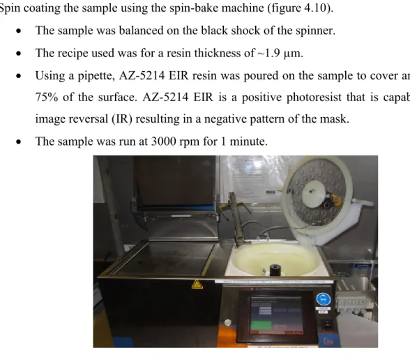
Figure 4.10: Spin-bake machine ... 39

Figure 4.11: Alignment marks ... 40

Figure 4.12: E-beam thermionic evaporation machine ... 41

Figure 4.13: Magnetron sputtering machine ... 43

Figure 4.14: Kapton tape ... 43

Figure 4.15: Plasma asher machine ... 45

Figure 4.16: Reactive ion etching Oxford (RIE) ... 46

Figure 4.17: Etched holes circled in red... 46

Figure 4.18: Phase diagram for carbon dioxide and water... 47

Figure 4.19: CPD machine chamber lid ... 48

Figure 4.20: Spacers are used to minimize the chamber volume ... 49

Figure 4.21: CPD control panel ... 49

Figure 4.22: LCO2 filling the chamber ... 49

Figure 4.23: LCO2 and IPA mixture ... 50

Figure 4.24: In the purging step, the IPA is drained out of the chamber and LCO2 is filling the chamber. ... 50

Figure 4.25: At the end of the purging step, the chamber is filled with pure LCO2. .... 50

Figure 4.26: The chamber is kept at critical point conditions. ... 51

Figure 4.27: the CO2 gas exhausted out of the chamber. ... 51

Figure 4.28: Bain Marie used for lift-off with ultrasound waves ... 53

Figure 4.29: First four design layers on a rotatable mask. ... 54

Figure 4.30: Second four design layers on a rotatable mask. ... 54

Figure 4.31: (a) is the sacrificial layer for one CMUT cell, (b) are holes to reach the Cr sacrificial layer for each CMUT cell, (c) is the top electrode, and (D) is the complete CMUT cell. ... 54

viii

Figure 4.33: Deposition resolution of the chromium ... 55

Figure 4.34: Peeled membrane after sacrificial layer etching taken by SEM ... 56

Figure 4.35: Residual Cr after etching for more than 20 hours ... 57

ix

List of acronyms and abbreviations

CMUT Capacitive Micro-machined Ultrasonic Transducer

CPB Cardiopulmonary bypass

SIRS Systemic Inflammation Response Syndrome

LBUM Laboratoire de biorhéologie et d`ultrasonographie

médicale

LIOM Laboratoire d'imagerie optique et moléculaire

RBC Red Blood Cells Aggregation

US Ultra Sound

MODS Multiple Organ Dysfunctions

Rayl Rayleigh

Pb (Zr,Ti)O3 Lead Zirconate Titanate

PZT Lead Zirconate Titanate

BaTiO3 Barium Titanate

CaTiO3 Calcium Titanate

PVDE Polyvinylidene

LiNbO3 Lithium Niobate

AIN Aluminum Nitride

NDE Non-Destructive Evaluation

MEMS Microelectromechanical Systems

Si3N4 Silicon Nitride

Al Aluminum

Cr Chromium

RIE Reactive Ion Etching

CPD Critical Point Drying

UV Ultraviolet

HF Fluorhydric Acid

IPA Isopropanol

x

Au Gold

E-Beam Electron Beam

EBPVD Electron Beam Physical Vapor Deposition

LCO2 Liquid Carbon Dioxide

ESM Electron Scanning Microscope

xi

ACKNOWLEDGEMENT

First, I want to thank my parents, my family, and my friends for their support and encouragement throughout my studies. They have always motivated me to pursue my goals and to fulfill my ambitions.

A special thanks to my research supervisor, Dr. Guy Cloutier, for giving me the chance to do my graduate studies in his lab, and to my co-supervisor Dr. Frederic Lesage who gave the opportunity to work on this microfabrication project.

Also, a big thanks to Dr. Marie-Hélène Bernier and Christophe Clément, the responsible on the LMF Lab, who gave me all the needed trainings and help to continue in this work.

Finally, I want to thank all my colleagues in LBUM and LIOM for helping me directly or indirectly during my stay.

1

Chapter 1 Introduction

1.1 Medical Context

Inflammation is the tissue immune response to any infectious or non-infectious insult to restore organ or system functionality. Although the inflammatory response is usually advantageous and reversible, it can become excessive and uncontrolled [1]. Inflammation can be caused by different types of insults, like ischemia, trauma, chronic diseases, burns, infections, or pancreatitis [2]. The term sepsis is used to indicate an abnormal inflammation due to infection, whereas a similar inflammatory response can happen in absence of infection and can have the same mortality rate as sepsis, in this case the medical terminology used is the systemic inflammatory response syndrome (SIRS).

SIRS is a non-specific and spread inflammatory process in the body that is independent of causative factors of any sepsis state. It can evolve to advanced SIRS, sepsis, severe sepsis and septic shock [3]. The common complication of SIRS is the growth of organ dysfunction, including acute lung injury, renal failure, and multiple organ dysfunction syndrome (MODS) often cascading to sudden death [1]. Patients developing SIRS may also have long term consequences with a risk of death up to 5 years after the septic event [4].

Cardiac surgery can promote many deleterious events including SIRS. The Society of Thoracic Surgeons National reported a mortality rate of up to 41% in the 11% of patients developing MODS after cardiopulmonary bypass (CPB) [1]. The occurrence, severity and clinical outcome of the inflammatory response and reasons why certain patients develop complications after CPB is related to three factors.

First, the homeostatic control of the balance of pro- and anti-inflammatory cytokines can be deviated from normal balance in urinary, gastrointestinal or respiratory tracts, or in blood plasma because of the intense pro-inflammatory stimulus occurring during CPB. Changes in time, magnitude and pattern of cytokines release, to keep this balance, can cause abnormalities in the inflammatory response. When the inflammatory response becomes unbalanced, the liver releases molecular messenger proteins into the blood stream. Acute phase proteins, like fibrinogen, C-reactive proteins, ceruloplasmin and glycoproteins, increase the bounding

2

between erythrocytes leading to the formation of abnormal aggregates [5]. The large volume of aggregates increases the viscosity of blood. On the other hand, the over release of cytokines has a direct effect on the vascular tone resulting in a decrease of blood pressure. Both conditions make the oxygen transport into capillaries more difficult, which may decrease the end-organs perfusion [6, 7].

Second, a ‘multi hits’ model can occur, where MODS can be developed in less injured patients as a result of a reactivation of their inflammatory response caused by an adverse and often minor events in pre-hospital settings or in emergency room such as untreated pain, delayed fracture fixation and a complication of invasive monitoring. These insults are sometimes known as second hits and anyone of these insults can be a trigger to start the main inflammatory response to cause MODS over a period of time [1, 8].

Third, the pro-inflammatory response ‘SIRS’ is one side of the inflammatory response process, the other side is known as the inflammatory response or “compensatory anti-inflammatory response syndrome” (CARS), this is escalated by the body in response to the original inflammatory state. The pro-inflammatory and anti-inflammatory mediators are released because of an initial insult to achieve a homeostasis balance. These mediators can be considered as two opposite unbalanced forces. Initially, these mediators interact in the microenvironment of the tissue insult site. The homeostasis is achieved if mediators balanced each other and overcome the initial insult. If not, the mediator interaction is expended and also occurs into the systemic circulation. If a balance is not achieved at this level and homeostasis is not restored, a massive proinflammatory reaction (SIRS) or an anti-inflammatory reaction (CARS) will occur [9].

Currently, SIRS can be diagnosed by the presence of 2 or more of the following symptoms: • A fever of more than 38°C or body temperature less than 36°C.

• Heart rate of more than 90 beats per minute.

• Respiratory rate of more than 20 breaths per minute or arterial carbon dioxide tension (PaCO2) of less than 32 mmHg.

• Abnormal white blood cell count (>12,000/µL or <4,000/µL or >10% immature) [10]. However, considering these factors alone lack specificity because they can also be detected for other reasons than SIRS. An alternative way to diagnose SIRS is by using biochemical markers.

3

The analysis of more than 80 blood markers of inflammation can be done to detect this syndrome [11, 12]. Among relevant markers are proteins interleukin 6 (IL-6) [13], C-reactive (CRP) [2], tumor necrosis factor alpha “TNF-alpha”, and procalcitonin [14]. However, blood markers require venepuncture and laboratory analyses, which take time to get results to determine the presence of the inflammatory state.

Another blood test used to diagnose SIRS is the erythrocyte sedimentation rate (ESR) or Biernacki’s reaction. With this test, the rate of separation of red blood cells (RBCs) from the plasma is tested. In the presence of inflammation, the blood separation is faster than in the normal state because large RBC aggregates sediment more rapidly than individual RBCs. A few drawbacks exist with this method. First, it is time consuming as it takes around 1 hour to get the measurement. Second, due to difficulties in distinguishing between sedimentation levels of non-pathological samples, the measurement is lacking sensitivity. Third, ESR strongly depends on the hematocrit and the viscosity of the plasma, which are confounding variables.

Many other tests besides ESR, can be done to quantify RBC aggregation to interpret the inflammatory state. The zeta sedimentation ratio (ZSR) has the advantage over ESR of being faster and insensitive to hematocrit differences, but as ESR, this method can estimate the RBC aggregation but not the time course of the process. Moreover, it is also dependent of the plasma viscosity, which is influenced by the presence of fibrinogen and gamma globulin [6]. The low-shear viscometry method is used in research and it consists of using an instrument capable of applying different shear rates to a blood sample to indirectly detect the influence of RBC aggregation. The RBC deformability and plasma viscosity can affect the measurement with this method [6]. A microscopic aggregation index (MAI) has also been used to assess RBC aggregation using a blood smear and a camera coupled to a microscope. As for the ESR and ZSR, this method can estimate the amount of RBC aggregation but not the time course of the aggregation kinetics. Moreover, it is time consuming because of the manual counting of cellular units by direct observation or by using microphotographs or video images [6]. A method as in the MAI measure relies on an image analysis technique. The average number of RBCs per aggregate is used to quantify aggregation using a microscopic image analysis software and flowing blood into a microfluidic system. This method is estimating the volume of each RBC aggregate; dividing this by the volume of each RBC allows obtaining the mean aggregate size [6].

4

Photometric methods have also been developed and are today considered gold standard approaches to measure RBC aggregation in research protocols. With this method, the measurement of RBC aggregation relies on the light transmission and/or reflection over a blood film or a thin layer of circulating blood into a Couette device. Under low shear condition, the RBCs form rouleaux and this aggregation creates gaps between aggregates. The light transmittance or reflection is a function of the effective average of these gaps and therefore is indicative of the degree of aggregation. The photometric method measurements can be affected by a few factors. First, as for any other in vitro laboratory instrument methods, the temperature can affect the RBC aggregation during the measurement. Second, the RBCs should be fully disaggregated at the beginning of measurements to avoid any memory effect (i.e., an initial state with residual aggregates). Third, the oxygenation of the sample can affect the measurement by affecting the hemoglobin absorption of light [6].

All above mentioned techniques require having blood samples, and take time to get the result from laboratories, and most of them can estimate RBC aggregation but not the time course of the process.

1.2 Ultrasound Backscattering

A recent work done by our team showed the method and advantages of using ultrasound signal backscattered by blood to determine RBC aggregation and indirectly the inflammation state of an individual [15, 16]. With this approach, results can be monitored non-invasively and continuously in real time without the need of blood samples.

The most frequent use and recognized application of ultrasound is for medical imaging. Ultrasound compared to other medical imaging methods, such as magnetic resonance imaging (MRI) and computed tomography (CT), has advantages since it is relatively cheap, does not require a large infrastructure, is non-invasive and non-irradiating. Ultrasound imaging devices can even be portable and moved on the bed side, used outside clinics and hospitals, and transported in ambulances. It is also providing real-time images for monitoring. In addition to imaging, ultrasound can also be used for drug delivery and therapeutic applications to treat problems, such as kidney stones [17].

5

As introduced above, US can be used to estimate RBC aggregation but it does not have the resolution to show directly and clearly flowing RBC aggregates. However, by analysing the backscattered US spectral properties from blood, RBC aggregates can be characterized. Four decades of research revealed that backscattered waves by RBCs are shear rate dependant and can be affected by the amount of fibrinogen or high molecular mass concentrations of other proteins known to modulate the level of RBC aggregation [16, 18]. This effect on backscattered waves is mainly due to the increase in particle volume associated with RBC aggregation [19].

In 2013, the first preclinical study on pigs to demonstrate the feasibility of monitoring the inflammation in real time using ultrasound methods was published by our team [13]. Later [20], it was shown that the backscatter coefficient (BSC) of blood at a mid-frequency of 35 MHz can present characteristics allowing discerning the erythrocyte aggregation level in humans by fitting the BSC to a spectral scattering model. Measurements were performed by controlling the blood flow by applying a force on the forearm, over the medial antebrachial vein, to have a low flow condition promoting reproducible measurements of RBC aggregation.

1.3 Project objective

This project is situated in a larger endeavour that aims to develop a portable high-frequency ultrasound system that integrates a detection system based on capacitive micromachined ultrasonic transducers (CMUTs) with signal processing algorithms to estimate RBC aggregation in superficial veins. In this work, the focus is on the design of CMUT transducers, starting from simulations to fabrication and then validation. The overarching

objective is to simulate, design, fabricate and validate a CMUT array of small size so that it can

be attached on a patient’s arm to continuously monitor RBC aggregation during cardiopulmonary bypass surgeries.

This project was realized in three steps:

1. Simulate and design CMUTs optimized to emit and receive over a large bandwidth with a central frequency of 40 MHz.

2. Develop a process to fabricate the designed transducers.

6

1.4 Thesis organization

This thesis is dedicated to the simulation and fabrication of the CMUT array transducer. Chapter 2 presents a literature review on US transducers, including piezoelectric transducers and CMUTs. Chapter 3 follows by giving the details on the CMUT analytical modeling of the collapse voltage and the resonant frequency. This chapter then presents the simulation of one CMUT cell using COMSOL and the design of CMUT arrays. Finally, using the CMUT designed arrays, an ultrasound beamforming simulation using FIELD II is presented to demonstrate theoretically the performance of the system. Chapter 4 focuses on some fabrication methods used in the past for CMUT, and the sacrificial releasemethod adopted in this work. Finally, chapter 5 includes the discussion of results and a conclusion on works done.

7

Chapter 2 Ultrasound Transducer Literature Review

2.1 Piezoelectric Ultrasound Transducer Technology

Since the discovery of piezoelectricity by the Curie brothers in 1880, the piezoelectric effect and associated materials became the most relevant technology for US production among other explored transduction mechanisms. The fundamental basics of piezoelectric transducers include crystal generating a voltage when it is exposed to mechanical pressure, known as the direct piezoelectric effect, and vice versa when a voltage is applied to a piezoelectric material to deform and vibrate it, known as the converse piezoelectric effect. Thus, when it is applied to a medium supporting wave propagation, the pressure signal can be controlled by the applied voltage.

There are many types of materials and fabrication processes that can be used to produce US transducers. Initially, single crystal natural materials such as quartz and Rochelle (potassium sodium tartrate tetra hydrate) salts were used for this purpose. However, the piezoelectric effect in such materials is weak and although they formed the basis of transducers for underwater sonars, non-destructive evaluation (NDE) testing and early biomedical applications, the performance improved significantly with the invention of ferroelectric materials in the 1950s. Examples of such materials are lead zirconate titanate Pb (Zr, Ti) O3 and barium titanate (BaTiO3). Another more recent ferroelectric material is calcium titanate (CaTiO3), which has better performance by adding dopants to it. The name ferroelectric was given for these materials because of the types of properties they share with ferromagnetic materials, not because of a link with iron. The main ferroelectric material property is its finite electrical polarisation with or without the application of any external electrical field. One of the best examples of a ferroelectric material is barium titanate, which was originally a paste that was dried and sintered, and then mixed with a liquid to take the lightly bounded crystalline grains shape, then these grains will be divided and rearranged by itself regarding its own polarisation. [21]

In general, there are four types of piezoelectric materials: piezoceramics, piezocrystals, piezopolymers and piezocomposites (see Table 1). Currently, the most used piezoelectric materials are piezoceramics (PZT). PZT has a hexagonal symmetry crystallography shape; they

8

are available in hard (PZT-4) and soft (PZT-5H) types. PZT-4 is used in applications where high intensity ultrasound is required, whereas PZT-5H is selected in applications where higher sensitivity due to better piezoelectric performance is needed. PZT-4 and PZT-5H are currently used in many applications but other ceramics are available for specific needs, for example lead metaniobate (PbNbO3), which is used in high temperature applications and where broad frequency bandwidth is required [21].

The second type of piezoelectric materials is piezocrystals; they were the first piezoelectric materials, but they were rapidly replaced by PZT. Lithium niobate (LiNbO3) and aluminum nitride (AlN) are widely used piezocrystal materials. LiNbO3 has a lower symmetrical crystallographic shape than PZT, and higher than the piezopolymer polyvinylidene (PVDF). LiNbO3 is used for high frequency applications because of its low losses and high longitudinal propagation speed. It is also a good material for high temperature applications. AlN has the same crystallography as PZT and the same characteristics as LiNbO3. AlN is characterized by its crystalline thin film form, which makes it useful for surface acoustic wave devices and in NDE applications [21].

The third type of materials used to fabricate ultrasound transducers is piezopolymers. The most commonly used piezoelectric polymer is polyvinylidene (PVDF), which has a thin plastic film form. This material has a low symmetrical crystallographic shape because axial stretching is used instead of an electrical field for polarising it during fabrication. Material properties make them very useful for broadband receivers in underwater detection applications and high-frequency medical imaging [22].

The last type is made of piezocomposites. This material consists in several piezoelectric ceramic particles bounded all together by a polymer matrix. Piezocomposites are used in applications where there is a mismatch in acoustic impedance between the transducer and the propagation medium, e.g. for underwater detection, NDE and biomedical imaging. The reason of using composite materials bounded by a polymer is the capability to achieve lower acoustic impedances in low acoustic impedance media, and the fact that this composite material decreases the US propagation amplitude in the lateral direction [21].

9

Table 1: Properties of selected piezoelectric materials, this table is reproduced from Table 1.2 of [21]

2.2 Capacitive Micro-Machined Ultrasonic Transducers

Capacitors have been used as alternatives to piezoelectric materials in some acoustic applications, like microphones in audio applications. The French physicist Paul Langevin predicted that capacitors could be a substitute to piezoelectric materials if a high electric field is produced across capacitor plates to force them to vibrate [23, 24]. During World War I Langevin built the first electrostatic capacitor transducer with large plates gap, for echo-ranging experiments in water but later he replaced it with quartz piezoelectric transducers [25].

With capacitive micromachined ultrasonic transducers (CMUTs), a different physical principle is used to generate ultrasound based on electrostatic forces. CMUTs consist in a flexible membrane design made at a very small scale via a micromachining approach on silicon wafers. Generally, two voltages (DC and AC) are applied on top and bottom electrodes to generate electrostatic forces and actuate the membrane. The notion of electrostatic forces to generate membrane movement is not a new discovery; the concept was developed as early as piezoelectric transducers. In 1900s, capacitive transducers were first discovered and fabricated with large air gaps by Langevin for condenser microphone applications [26] . Until 1980s, early CMUTs were used for small condenser microphones [27] and pressure sensors [28].

To have a good performance compared to piezoelectric transducers, the electric field generated in the CMUT should be very high, in range of 108 _{V/m, which in turn requires a very} small gap between transducer plates. With the development of micro fabrication techniques, in the early 1990s, scientists were able to fabricate micro capacitors with very small gaps that made this possible. In 1994, the first CMUT was fabricated on a silicon wafer by a Stanford University group, lead by Prof. Yakub Khuri [29], where a standard micromachining technique was used to build an electrostatic transducer that could operate at 1.8 MHz and 4.6 MHz. Since that time,

10

low and high frequency CMUTs were fabricated [30, 31] and used in many applications, such as air coupled transducers [29] and non-destructive evaluations [32], where it was shown that there is no need to use liquid coupling fluid with the CMUT to improve the impedance mismatch between the transducer and air, as in piezoelectric transducers for non-destructive evaluation. In [33], two CMUT designs were used to measure the wind speed using the amplitude of the signal and the time of flight method. For gas sensing [34], two CMUTs facing each other were built, where the gas flows in between and the CMUTs measure the variation of the ultrasonic velocity and attenuation than by inverse problem the gas concentration is measured. After air-coupled applications, CMUTs were used widely in medical imaging and therapy applications [35]. In the latter report, authors showed advantages of using CMUTs for conventional 2D cross-sectional imaging by building a 128-elements 1D array using the wafer bounding process. The fabricated transducer operated at a central frequency of 7.5 MHz and had a 100% fractional bandwidth. This CMUT transducer showed better resolution and better definition of fine structures in the carotid artery and thyroid gland compared with an equivalent piezoelectric transducer. In the same article, authors showed the possibility of using CMUT as a therapeutic tool.

The general structure of a CMUT consists of two electrodes covered by an elastic membrane, usually made of silicon, separated by a small vacuum gap. This membrane vibrates and produces ultrasound when transient voltages are applied on the electrodes. (See figure 2.1)

11 Two types of CMUT operation have been described:

1) The conventional CMUT, where the upper membrane is free to vibrate under the electrostatic actuation by the electrodes.

2) The other CMUT operation is the collapse mode, where a DC voltage is applied to collapse the upper membrane until it touches the center of the lower membrane. With the application of an AC voltage, the annular free part of the upper membrane vibrates leading to an increase in operation frequency associated with the higher membrane vibrational mode.

At equal frequency, the collapse mode CMUT has two main advantages over the conventional CMUT, which are the wider bandwidth and the better output pressure sensitivity [36]. Semiconductor fabrication techniques are used for CMUT production. These techniques have proven to be precise, highly reliable and repeatable. CMUTs thus have high device stability, good dimension control and good reproducibility, with inexpensive production cost when mass-produced. Since all dimensions are patterned simultaneously on a wafer, array fabrication does not introduce significant expenses. The design control for CMUTs is achieved through photolithography, which is highly scalable to be fabricated in micro dimension. A wide range of geometries can be fabricated, resulting in devices covering a wide operating frequency range. Moreover, they can be coupled to integrated circuits (IC). Another characteristic is the higher resolution of CMUTs as the wider bandwidth over piezoelectric transducers allows covering upper frequencies [35]. In air or immersion applications, CMUT does not need for matching layers because the low impedance of CMUT thin membranes is lower than those of air and water [37, 38].

Another advantage of CMUT is that it can be used in high temperature applications such as car exhausts for gas detection, where silicon, silicon nitride and silicon oxide can sustain high temperature range (< 800o_{C). In comparison, piezoelectric transducers are not possible in high} temperature applications because the transducer material is losing its piezoelectricity. Also, in high intensity focused ultrasound therapy applications, the piezoelectric component needs to be cooled down by water because of heat produced by dielectric loss, whereas with CMUT, the silicon substrate absorbs and distributes the heat faster because of its good thermal conductivity [39]. Another application where CMUTs can be used easier than piezoelectric transducers is for

12

magnetic resonance imaging (MRI) applications, because CMUTs can be fabricated from materials not affected or not affecting the magnetic field of the MRI system. For this reason, CMUT transducers can be used for MRI guided therapeutic procedures [40].

The major disadvantage or limitation that CMUTs have is the low output pressure [41]. Ultrasound waves cannot penetrate well into structures when the transducer has a low transmitted pressure, especially in medical applications where access to deep organs is important. Specific designs where several CMUT elements are activated simultaneously can help increasing the transmitted pressure. Sensitivity can be improved in collapse mode CMUT and in conventional CMUTs by using a metal mass in the membrane center [42].

With all these advantages of CMUT, PZTs are still used because of the ease to manufacture in millimetre sizes, and because they still have higher working frequencies and higher output pressure that provide better image quality and stability [43]. In the opposite side, piezoelectric transducer fabrication is labor intensive, expensive, and suffers from large manufacturing variability.

13

Chapter 3 Capacitive Micromachined Ultrasonic

Transducer Design

Prior to initiating micro-fabrication, CMUT parameters as geometrical dimensions are usually determined by modeling and simulations. This chapter introduces the analytical modeling of CMUT, using a lumped electro-mechanical circuit model. Using that model, the collapse voltage and the resonance frequency were derived with respect to the radius and the material properties of the CMUT’s membrane. Then, COMSOL simulations were performed on a CMUT cell to better specify the transducer function and performance using all membrane properties. Finally, CMUT arrays were simulated using FIELD II to characterize ultrasound (US) beam forming characteristics.

3.1 CMUT operation and modeling

With CMUTs, the transmitted US and the received voltage are generated by the electrostatic physical principle and not by material properties. As described before, by applying a transient electric field across two parallel plates, US waves are generated due to the plates’ vibration associated with forces due to charge accumulation and the inverse is also true. When the plates receive US waves, they vibrate to generate voltages that can be read out and processed to images. To simplify analytical modeling, one can initially assume that the CMUT element consists of two parallel circular plates without any insulation layers. Membranes thus play the role of electrodes as well as vibrating components. Furthermore, the CMUT is assumed to be operating in vacuum with no load on membranes, and the acoustic damping is assumed to be null.

The analytical model of a CMUT introduced in [44] was implemented based on a lumped electro-mechanical model, as shown in figure 3.1.

14

Figure 3.1: lumped electro- mechanical model

In this model, mass represents the mass of the CMUT membrane, the capacitor corresponds to the capacitance of the CMUT, and the spring describes the elasticity of the membrane. The transformation of the electrical energy to acoustical energy in the CMUT is represented by damping in this model and the mass is actuated by the forces of the spring and the capacitor.

F

+

F

=

F

By differentiating the potential energy of the capacitor with respect to the position of the mass (or membrane), the force exerted by the capacitor FCapacitor is given by the equation (3.2).

(

)

where: C is the capacitance,

V is the the applied voltage across the capacitor,  is the permittivity of the free space, 0 A is the surface area of the capacitor,

d0 is the effective gap distance between top and bottom electrodes, and

x is the displacement of capacitor plates in positive direction from equilibrium. The restoring force of the membrane, which is represented by the spring force Fspring, is

linearly proportional to the displacement x, as shown in equation (3.3).

spring

15

where k is the spring constant of the capacitance membrane. The spring constant for a CMUT membrane that has a circular shape clamped at boundaries is obtained from[45]:

(

)

where: E is the Young’s modulus of the membrane material,

dm is the membrane thickness,

R is the membrane radius, and υ is the Poisson’s ratio.

Figure 3.2: CMUT circular plates clamped on the edges

Figure 3.2 shows the CMUT circular plates with radius R clamped on edges and deflected under a uniform pressure created by the electrical force.

The result of the spring and capacitor forces is the mass force, Fmass, and it can be

represented by the following equation where t indices time:

( )

Putting all forces in equation (3.1) give the time dependent equation of the system:

16

( )

( )

( )

(

)

( )

3.1.1 Collapse voltage calculation

By considering V(t) = VDC, harmonic terms are eliminated from equation (3.6) and the

equation becomes simpler yielding:

(

)

By solving equation (3.7) as a third-degree linear polynomial in x, the pull in voltage or collapse voltage can be represented in equation (3.8). In this project, equation (3.8) is used to determine the collapse distance of the membrane for the design and simulation. After the transducer fabrication, equation (3.8) can be used to analytically calculate the collapse voltage and to compare it with the measured collapse voltage.

3 0 0 8 27 collapse kd V A  = (3.8)

By substituting equation 3.8 into equation 3.7, one can get the displacement of the membrane at the collapse state, dcollapse.

0 2 3

collapse

d = d (3.9)

Since the area of the circular membrane is: 2

A=R , (3.10)

substituting equations 3.4 and 3.10 into 3.8 give:

(

)

3.1.2 Resonant frequency calculation

17 0 0 1 2 k f M  = (3.12)

where f0 is the resonant frequency, k is the spring constant, and M0 is the effective mass of the

membrane or the equivalent mass of the lumped model. The effective mass of the membrane can be written as [45]:

( )

where ρm is the density of the membrane material and (λa)mn is a constant corresponding to the

mode shape of the membrane. For a membrane vibrating at its fundamental frequency, (λa)mn is

(λa)00 = 3.196 [46]. Putting equation 3.4 and 3.13 into 3.12 give:

( )

(

)

3.2 COMSOL simulation

While previous equations provide a good description of the CMUT system, simulations are required in the case the membrane consists of more than one layer. In this project, the targeted frequency was 40 MHz. To have exact dimensions of the CMUT cell thickness and radius, and to choose the best materials to obtain the needed frequency, reliable finite element analysis software was needed. COMSOL Multiphysics v5.2 was chosen because of its easy graphical interface and the ability of using different modules to simulate MEMS designs like CMUT.

3.2.1 CMUT cell setup

After iterating through a few designs, the CMUT membrane radius used for simulating the 40 MHz element was 20 μm and other parameters are shown in Table 1. The resonant frequency is determined by the CMUT radius, the thickness of the layers and the material used for the membrane and for the electrodes. The material properties are shown in Table 2.

18

Table 2: CMUT cell dimensions

Vibration part of

the transducer

Membrane layer, Si3N4, 0.3 μm

Top electrode, Al, 0.1 μm Membrane layer, Si3N4, 0.3 μm

Vacuum gap, 0.3 μm

Isolation layer, Si3N4, 0.3 μm

Bottom electrode, Al, 0.1 μm

Table 3: Materials properties used in COMSOL

In the simulation of the CMUT cell, one cell was modeled in 2D-axisymmetric dimension to facilitate the drawing of the collapsed membrane and for faster simulations. From the MEMS module, the Electrostatics, Solid Mechanics and Moving Mesh physics were used to calculate the eigen frequency.

Figure 3.3: Cross section of the CMUT cell in 2D

The red layers in figure (3.3) are the top and bottom electrodes, where the AC and the DC voltages are applied. This AC voltage aims to vibrate the membrane (grey layers) to produce US. As mentioned before, three modules were used, and every module has its own boundary conditions that were applied on CMUT layers.

Electrostatic conditions were applied on all layers except for the electrodes (red layers)

because it is not necessary to solve for the potential in the electrodes since it is constant. The Si3N4 Aluminum

Young's modulus ( Gpa) 250 70

Relative permitivity 9.7 1

Density ( Kg/m^3) 3100 2700

19

bottom red layer was set to be the ground (V = 0), and the electric potential boundary was applied on the top red layer (V). Zero charges were set on boundaries shown in figure (3.4); this means that there was no surface charge accumulation on these boundaries and that the electric and displacement fields were blocked across these boundaries. Finally, the force calculation domain was set to membrane layers (grey layers in figure 3.3), so the software used Maxwell’s stress tensor over the exterior surface of selected layers to calculate electromagnetic forces by integrating equation (3.15) on the surface of selected layers. This equation is given by:

(

) (

)

where n1 is the outward normal from the layer, E is the electric field, and D is the electric

displacement, T2 is the force per unit area at a surface.

Figure 3.4: Zero charge boundaries

In solid mechanics, a fixed constraint boundary condition was applied on some boundaries to avoid deformation during the vibration of the membrane.

By default, all boundaries in Comsol are “Free” (i.e. free to move). Applying the fixed constraint boundary condition on the blue parts shown in figure (3.5) will prevent them from moving and will keep them in a collapsed position as they are designed, where the other part of the membrane vibrates.

The radius of the collapsed area was estimated based on [47]. In the present work, for a membrane radius of 20 μm, a collapsed area radius between 8 μm and 10 μm was chosen.

Figure 3.5: Fixed constraint boundaries

Then the boundary load was used to apply traction or pressure to the lower boundary of the membrane, where all the load pressure created by the electric field takes place (see figure

20

3.6). Then, the load was defined as a force per unit area, so COMSOL took the value of the total force per unit volume and divided it by the thickness.

Figure 3.6: Boundary load

The moving mesh condition was applied on all CMUT layers. This module was used to maintain the equilibrium between the electric field finite elements and the mechanical deformation. The mesh generated is shown in figure (3.7). The membrane was meshed to many elements. Those elements are calculation points used by COMSOL to give the output. An increased number of calculation points correspond to more output but at the cost of higher computation time. To make sure that meshing was sufficient and enough to yield precise results, many runs were done with finer meshing in every run, until the change in results was very small. The calculation was slower with every finer mesh run, which required an increase in computer memory to be able to finish the simulation.

Figure 3.7: Mesh generated

3.2.2 COMSOL simulation results

As a first step, we reproduced a simulation from the literature [48], where the design was simple: the top electrode and the insulation layer were not included in the analytical modeling nor in the simulation. This step served to validate that the simulation was generating expected frequencies. So, to validate our work, the analytical calculation and the COMSOL simulation were done without the top electrode, the insulation layer and in conventional mode. Then, analytical results were compared with COMSOL results.

After placing material properties and CMUT dimension parameters of [48], i.e., properties in table 3 into equation (3.14), the resonant frequency obtained was 5.85 MHz, which is equal to what the author got in [48] as shown in figure (3.8). The simulation of the CMUT

21

given in [48] was repeated using COMSOL and results are shown in figure (3.9). Again, the resonant frequency obtained was equal to that of author’s simulations, with small differences around 0.411% between analytical and simulation results.

Table 4: CMUT parameter values used in this project and in [48]

Symbol Reference CMUT values This project CMUT values

E 160 GPa 250 GPa ν 0.23 0.23 (λa)00 3.196 3.196 m  2332 kg/m3 _{3100 kg/m}3 0  8.854x10-12_{F/m 8.854x10}-12_F/m dm 1.5 μm 0.6 μm 0 d 0.75 μm 0.3 μm Radius 32 μm 20 μm

Figure 3.8: The analytical relationship between the membrane radius and the resonant frequency in [48]

Figure 3.9: COMSOL CMUT simulation considering parameters of [48]

22

In a similar way, by repeating the analytical calculation using equation (3.14) with CMUT parameters given in table 3, the resonant frequency obtained was 6.49 MHz, as seen is figure (3.10). Furthermore, the same COMSOL simulation was done for the CMUT without the top electrode and the insulation layer with a membrane thickness of 0.6 μm and results are shown in figure (3.11).

Following validation of the COMSOL simulation with the literature, we gained confidence that steps followed on COMSOL would provide accurate results. So, the next step was to simulate a collapsed mode including all CMUT layers. According to the analytical calculation and using the simple CMUT without the top electrode, the radius had to be 8.06 μm to have a frequency of 40 MHz, see figure (3.12). To have the same frequency in collapse mode with the top electrode, the COMSOL simulation predicted requiring a 20 μm membrane radius. The difference in radius between COMSOL simulations and analytical results for a 40 MHz frequency CMUT is due to the additional 100 nm electrode layer made of aluminum and the collapse design used in COMSOL simulations. In the collapsed mode simulation not all of the membrane (20 μm) radius will vibrate, as shown in figure (3.13). The middle circular surface is fixed and only a part of the 20 μm radius is vibrating in a “donut” shape.

Figure 3.10: The analytical relationship between the membrane radius and the resonant frequency for our CMUT design.

23

Figure 3.12: Analytical simulation for a 40 MHz CMUT element

The goal of simulating with COMSOL is to get the resonant frequency or the eigen frequency of the CMUT. The first and second eigen frequencies are shown in figures (3.13) and (3.14). One needs to mainly consider the first eigen frequency that represents the transducer resonant frequency. Other frequencies are not useful because they would produce irregular shapes of the membrane and a non-stable transducer pressure. These, secondary simulated frequencies are avoided by exciting the transducer with specific pulses to generate the 40 MHz frequency.

The red color in figures (3.13) and (3.14) represents the large displacement area of the CMUT membrane, and the blue color represents less displacement areas.

24

3.3 Unit design

Every unit of CMUTs has the form of two groups of 6 x 128 CMUT cells that emit US separated by 16 x 64 CMUT cells that receive US. As shown in figure (3.15), (a) are the emitter parts of the transducer and (b) is the receiver part, and figure (3.16) shows the CMUT cells connected to form arrays with 8 holes around the membrane shown in green color.

The transducer array is designed to have a center frequency of operation of 40 MHz. To avoid grating lobes, the element pitch, which is the distance between two CMUT cells centers, should be less than half a wavelength (19.25 μm). For the CMUT presented in this dissertation, the element pitch was chosen to be 56 μm. This is mainly for design and fabrication purposes, to keep space for the wiring connections between the CMUT cells and for the holes which will be use for sacrificial release in the fabrication step.

The receiver column was designed to be shorter than the emitter columns, to minimise as much as possible the lobes artifacts. In this way the transducer will be focused to receive the main beam of the reflected US waves without the grating and the side lobes.

25

Figure 3.15: CMUT units, (a) the emitter cells, (b) the receiver cells

Figure 3.16: Zoom on the CMUT array with the sacrificial holes and channels shown in green

3.4 FIELD II simulation

To have an idea about the US beam formed by the CMUT design of figure (3.15), a simulation of the US field was done using the Field II Ultrasound Simulation Program [49]. This simulation can help to find the final design of the transducer and the distribution geometry of CMUT cells. (for the FIELD II code see appendix A)

Field II is a toolbox with pre-defined functions that can be used with MATLAB. All simulations were done by writing MATLAB codes or making changes on the existing Field II codes. The first step was to build the CMUT transducer geometry shown in figure (3.16), set up the simulation environment (center frequency, pulse length, etc …), then generate transmit and receive apertures, setting up the impulse response and the excitation. Finally, a measurement point in space was defined, the blue line shown in figure (3.18), to determine the pressure and the sensitivity of the receiving transducer.

26

Figure 3.17: CMUT design built in the FIELD II environment

-1.5 -1 -0.5 0 0.5 1 1.5 -1 -0.5 0 0.5 1 -2 -1.5 -1 -0.5 0 0.5 1 1.5 2 z [m m ] x [mm] y [mm]

27

Figure 3.18: FIELD II Measurement points (Blue), (a) Top View (b) Side View

3.4.1 Field II simulation results

The US transmitted beam is shown in figure (3.19), the dark red parts on the figure are the emitter CMUTs columns (a) previously shown in figure (3.15). the waves emitted from the two columns are combined to form the beam in the middle, where side lobes are created on the sides of the main beam.

The received pressure beam from the defined measurement points in FIELDII is shown in figure (3.20); the beam is well symmetric with no side lobes. The part (b) of figure (3.15) received the emitted beam without the side lobes created in the transmitted wave shown in figure (3.19). The combination of transmitted and received fields is the pulse-echo response shown in figure (3.21).

28

Figure 3.21: Pulse-echo response field

29

Chapter 4 CMUT fabrication

Since the early development of CMUT, many methods were proposed and used to fabricate these devices. The two major methods used are the sacrificial release micromachining technique and the fusion bonding technique or wafer bounding.

The first method used to fabricate CMUTs and for many years recognized as the standard fabrication process is the sacrificial release method [50]. After a decade, the fusion bounding technique was reported as a new fabrication method in the early 2000’s [51]. Over the years, many modifications were done on these two methods to report new fabrication processes. Some of the modifications reported for the sacrificial release technique are the polyMUMPS process [52] and the reverse fabrication process [53], the anodic bounding [54] and LOCOS[55] are examples of the modification reported for the wafer bounding technique.

It would be difficult to go through all fabrication techniques, but this chapter gives a general background on the wafer bounding technique and details on the surface micromachining method used in this project.

4.1 Surface micromachining method

The CMUT fabrication based on the surface micromachining method has been studied and used since its initiation in 1996 [29]. Over the years, some changes in the method of using the sacrificial release process in terms of materials used were reported by different researchers. However, a general idea for the standard fabrication process can still be described.

The first challenge in fabricating CMUTs is to obtain a cavity structure that allows the membrane to vibrate. With this technique, structures are patterned and deposited layer by layer, as shown in figure (4.1). It starts with a doped silicon wafer to be the bottom electrode of CMUTs. Then, the next step is to deposit the insulation layer (figure 4.1.a), which can be deposited by chemical vapor deposition (CVD) or by grown oxidation if the desired material is silicon oxide (SiO2). This layer is used in CMUTs to avoid shorting or to serve as an etch stopper in case the sacrificial layer material is etched with high selectivity. Depositing the insulation layer is a very critical point in CMUT fabrication because if the insulation layer has poor quality, this can create pinholes that may let the etchant in next steps to reach the substrate and etching

30

it. For this reason, a good quality deposition is needed such as low-pressure CVD (LPCVD) [56].

The next step is patterning and depositing the sacrificial layer shown in figure (4.1.b). The quality of this layer is not very important because it is removed later and is not needed in the final CMUT device. So, it can be deposited at a low temperature by CVD. What is important in this step is to choose a sacrificial material that can be etched with high selectivity against the insulation layer and the vibrating membrane, because the sacrificial layer is in direct contact with these two layers.

The third step is depositing the membrane (figure 4.1.c). The mechanical properties of the membrane are very important because it is the vibrating part of the CMUT, and it is responsible for generating US. It must be at a uniform thickness and with high quality deposition. For these reasons, a high temperature deposition process is preferable. Another important factor to consider during membrane deposition is the residual stress. A high residual stress can peel or collapse the membrane after release, which would make the device worthless. Thus, it is important to use a deposition method that allows controlling thin film stress levels during deposition, such as plasma enhanced CVD [57].

After membrane deposition, release holes that later allow the etchant to go through and reach the sacrificial layer are patterned and dry etched (figure 4.1.d). A high aspect ratio is needed for release holes, so an anisotropic etching method is used like the reactive ion etching (RIE) method. After this step, the wafer is dipped in an isotropic sacrificial layer etchant. The etchant should be isotropic to reach all areas under the membrane through the holes for releasing it (figure 4.1.e). To close the holes, another layer of the same material as the membrane can be deposited and added to the previous membrane, or a new layer can be patterned and deposited to close just the holes. In this case, the process is more complicated, and it requires the use of lithography and etching again, which can affect the membrane quality (figure 4.1.f).

The final step consists in depositing the top electrode and etching to allow the contact with the bottom electrode made of doped silicon. The bottom electrode contact holes can be dry or wet etched, after that the metal top electrode can be patterned and deposited (figure 4.1.g).

31

a) Insulation layer deposition b) Sacrificial layer deposition

c) Membrane layer deposition d) Holes etching

e) Sacrificial layer etching f) Holes sealing

g) top electrode deposition and bottom electrode hole etching

32

4.2 Wafer bounding method

In 2003, the wafer bounding technology was first used for CMUT fabrication at Stanford University [51]. This method provides more flexible CMUT designs because it is done using two wafers, one serving as the cavity and the other acting as the membrane, so design parameters of the cavity and membrane can be separately improved. Another advantage of this method is its simplicity. Indeed, fewer masks are needed compared with the sacrificial release method and less deposition steps are used.

The simple wafer bounding process starts with having two wafers, one is a silicon-on-insulator (SOI) wafer that serves as the membrane, and the second is a doped silicon wafer acting as the bottom electrode of the CMUT. The first step is growing oxide on the second wafer to serve as insulation layer of CMUT cells (figure 4.2.a). Cavities are patterned and dry etched on the grown oxide (figure 4.2.b). The third step is bounding the SOI wafer and the cavities wafer using a bounder under vacuum (figure 4.2.c). Then, bounded wafers are hardening at a high temperature to strengthen the bound. Using grinding and wet etching, the handle part of the SOI is removed and the oxide part also is removed using oxide etchant (figure 4.2.d). The next step is exposing bottom electrodes by dry etching, as shown in figure (4.2.e), then depositing top and bottom electrodes by sputtering or evaporation (figure 4.2.f).

33

c) Bounding the two wafers d) Removing the handle and the oxide parts

e) Dry etch to reach the bottom electrode f) Depositing the top and bottom metal electrodes

Figure 4.2: Wafer bounding process flow

4.3 Fabrication method used in this project

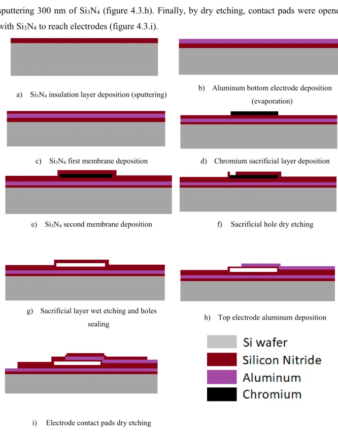
Considering advantages of the wafer bounding technique, the fabrication process used in this project is the sacrificial release method. Starting with a silicon wafer, a layer of 50 nm of silicon nitride (Si3N4) was deposited as insulator by sputtering to improve the adhesion of the first electrode on the wafer (figure 4.2.a). Then, the first electrode of aluminum (Al) (100 nm) was deposited by evaporation (figure 4.3.b), followed by sputtering a layer of Si3N4 (300 nm) as insulation layer (figure 4.3.c). After that, a layer of chromium (Cr) (300 nm) was evaporated to be a sacrificial layer (figure 4.3.d). That layer was covered by sputtering 300 nm of Si3N4 to be the first membrane (figure 4.3.e), and 8 holes were dry etched for every CMUT cell to remove the Cr by dipping the wafer into Cr etchant for 6 hours (figure 4.3.f). After this step, holes were

34

closed by sputtering a layer of Si3N4 (300 nm). The second electrode was deposited by evaporating 100 nm of Al (figure 4.3.g). It was then covered by the second membrane by sputtering 300 nm of Si3N4 (figure 4.3.h). Finally, by dry etching, contact pads were opened with Si3N4 to reach electrodes (figure 4.3.i).

a) Si3N4 insulation layer deposition (sputtering)

b) Aluminum bottom electrode deposition (evaporation)

c) Si3N4 first membrane deposition d) Chromium sacrificial layer deposition

e) Si3N4 second membrane deposition f) Sacrificial hole dry etching

g) Sacrificial layer wet etching and holes

sealing h) Top electrode aluminum deposition

i) Electrode contact pads dry etching

35

4.4 Fabrication process details

Fabrication is the most important and critical part to conduct after finishing simulations and having all dimensions of CMUT. Since the dimensions are in micrometers or less, CMUT needs to be fabricated in a clean room to minimize as much as possible dust particles that would defect the final product. (for the fabrication process see Appendix B)

Entering the clean room requires different trainings for personal and devices safety. Other trainings were also necessary for wafer preparation and for optimizing the fabrication process. Steps that were followed for the fabrication are photolithography for patterning, sputtering and E-beam evaporation for layer deposition, wet etching using specific etchants, lift-off and dry etching using reactive ion etching (RIE), removal of unwanted material layers and creating etching holes. In addition to plasma asher, critical point drying (CPD) and sample characterization using microscopes, and dektak stylus profiler to measure height variations of the substrate.

4.4.1 Safety in clean room

Before using any device in the clean room or starting any etching process, safety training on all fabrication equipment was given. Some of these devices can be mechanically or electrically dangerous and dangerous acids are used in a high temperature environment involving ultraviolet (UV) radiation. For all these reasons, very high safety measures were followed with professional trainers before taking any step forward (see figure 4.4).

36

Figure 4.4: Working with dangerous material certificate

4.4.2 Wafer preparation and cleaning

The first fabrication step is the wafer preparation and cleaning. Samples were fabricated on quarter wafer (figure 4.5), so every 5” the wafer was divided into four quarters using a diamond scribe (figure 4.6).

Then, quarters were cleaned from any organic or oxide materials using hydric fluor (HF) acid by dipping the wafer into HF for 30 sec, then rinsing it two times for 5 minutes each in water dump rinse (figure 4.7).

37

Figure 4.7: Water dump rinse

4.4.3 Photolithography

Photolithography, also termed optical lithography or UV lithography, is a process used in micro fabrication to pattern parts of a thin film or the bulk of a substrate. It uses light to transfer a geometric pattern from a photo mask to a light-sensitive chemical "photoresist", or simply "resist," on the substrate. A series of chemical treatments then either engraves the exposure pattern into or enables deposition of a new material in the desired pattern upon the material underneath the photo resist.

This step is very important and critical in the fabrication process because the goal is to have a good quality pattern and resolution that gives good deposition or etching later, so photolithography should be followed carefully specially for aligning and timing steps. Photolithography was repeated in all the layers fabrication. The type of photoresist, the developing time and the spinning speed were always the same, but the exposure time was changed every time depending on the UV lamp intensity.

The exposure time was set to 40 mJ divided by the lamp intensity (mW/cm2_{), which was} measured using a laser fluency meter before every layer alignment (figure 4.8). The steps followed for the photolithography are as follow:

38

Figure 4.8: Laser fluency meter

1. Washing the sample with acetone and isopropanol (IPA) to clean it from impurities or dust.

• The sample was sprayed with acetone for 10 to 15 seconds.

• For another 10 to 15 seconds, the sample was sprayed by IPA to rinse out the acetone and leave a clean surface.

• The sample was dried using N2.

2. The sample was vacuum baked using an oven to make sure that the sample surface was free from any water and liquid before applying the resin (figure 4.9).