A Real Option Approach to the Protection of a Habitat Dependent Endangered Species

Texte intégral

(1)2008s-30. A Real Option Approach to the Protection of a Habitat Dependent Endangered Species Skander Ben Abdallah, Pierre Lasserre. Série Scientifique Scientific Series. Montréal Décembre 2008. © 2008 Skander Ben Abdallah, Pierre Lasserre. Tous droits réservés. All rights reserved. Reproduction partielle permise avec citation du document source, incluant la notice ©. Short sections may be quoted without explicit permission, if full credit, including © notice, is given to the source..

(2) CIRANO Le CIRANO est un organisme sans but lucratif constitué en vertu de la Loi des compagnies du Québec. Le financement de son infrastructure et de ses activités de recherche provient des cotisations de ses organisations-membres, d’une subvention d’infrastructure du Ministère du Développement économique et régional et de la Recherche, de même que des subventions et mandats obtenus par ses équipes de recherche. CIRANO is a private non-profit organization incorporated under the Québec Companies Act. Its infrastructure and research activities are funded through fees paid by member organizations, an infrastructure grant from the Ministère du Développement économique et régional et de la Recherche, and grants and research mandates obtained by its research teams. Les partenaires du CIRANO Partenaire majeur Ministère du Développement économique, de l’Innovation et de l’Exportation Partenaires corporatifs Banque de développement du Canada Banque du Canada Banque Laurentienne du Canada Banque Nationale du Canada Banque Royale du Canada Banque Scotia Bell Canada BMO Groupe financier Bourse de Montréal Caisse de dépôt et placement du Québec DMR Fédération des caisses Desjardins du Québec Gaz de France Gaz Métro Hydro-Québec Industrie Canada Investissements PSP Ministère des Finances du Québec Raymond Chabot Grant Thornton Rio Tinto Alcan State Street Global Advisors Transat A.T. Ville de Montréal Partenaires universitaires École Polytechnique de Montréal HEC Montréal McGill University Université Concordia Université de Montréal Université de Sherbrooke Université du Québec Université du Québec à Montréal Université Laval Le CIRANO collabore avec de nombreux centres et chaires de recherche universitaires dont on peut consulter la liste sur son site web. Les cahiers de la série scientifique (CS) visent à rendre accessibles des résultats de recherche effectuée au CIRANO afin de susciter échanges et commentaires. Ces cahiers sont écrits dans le style des publications scientifiques. Les idées et les opinions émises sont sous l’unique responsabilité des auteurs et ne représentent pas nécessairement les positions du CIRANO ou de ses partenaires. This paper presents research carried out at CIRANO and aims at encouraging discussion and comment. The observations and viewpoints expressed are the sole responsibility of the authors. They do not necessarily represent positions of CIRANO or its partners.. ISSN 1198-8177. Partenaire financier.

(3) A Real Option Approach to the Protection of a Habitat * Dependent Endangered Species Skander Ben Abdallah†, Pierre Lasserre ‡ Résumé / Abstract Nous utilisons la méthode des options réelles pour déterminer quand un planificateur social doit interrompre ou reprendre l’exploitation d’une forêt, lorsque celle-ci constitue l’habitat stochastique d’une espèce menacée d’extinction. Le modèle présente des aspects économiques, écologiques et sociaux; il établit une règle optimale de gestion forestière qui fait l’arbitrage entre les bénéfices commerciaux de l’exploitation forestière et les risques d’extinction de l’espèce. Pour des paramètres correspondant au cas du Rangifer tarandus caribou, une espèce du centre du Labrador (Canada) menacée d’extinction, la politique optimale d’interruption et reprise de l’exploitation forestière est attractive; elle n’exige pas de longs arrêts dans l’exploitation, alors qu’elle réduit significativement le risque d’extinction et augmente la valeur de la forêt. Mots clés : options réelles, biodiversité, extinction, espèces menacées, aménagement forestier.. We use a real option approach to determine optimally when a social planner has to stop or resume logging in situations where an endangered species relies on forest habitat for its survival, and that habitat evolves stochastically. The model incorporates economic, ecological and social features, and is calibrated to generate an optimal forest management rule that balances the benefits from commercial forest exploitation with the risks of extinction facing the endangered species. For the reasonable parameters used in our application to the Rangifer tarandus caribou, an endangered species in Central Labrador (Canada), the policy of banning logging temporarily is quite attractive as it does not require long banning periods while it drastically reduces the extinction risk and increases forest value. Keywords: real options, biodiversity, endangered species, extinction, forestry. Codes JEL : C61; C63; D81; Q23; Q28 *. We are grateful to SSHRC, FQRSC, and the Sustainable Forest Management Network for .nancial support. We also thank the participants to the 17th Canadian Resource and Environment Economics (CREE) Annual Workshop, Ottawa 2007, the GAMM Annual Meeting, Zürich 2007, and the Agricultural and Resource Economics seminar at the University of Maryland, 2008. † Université du Québec à Montréal, ben_abdallah.skander@uqam.ca. ‡ Corresponding author : Département des sciences économiques, Université du Québec à Montréal, C.P. 8888, succursale Centre-ville, Montréal, Québec, Canada H3C 3P8. E-mail: lasserre.pierre@uqam.ca..

(4) 1. Introduction Commercially exploiting a forest which is home to some endangered species increases the later’s probability of extinction. A temporary ban on logging may prevent or delay extinction but implies foregone timber revenues. This paper uses real option theory to address these issues, with an application to the Rangifer tarandus caribou, an endangered species in Labrador, Canada. Caribous are a crucial component of the social, economic, and cultural lives of central Labrador’s Innus. As conservation measures, non-subsistence and subsistence hunting were prohibited respectively in 1972 and in 2002. Despite this protection e¤orts, the caribou population kept declining and was listed as threatened under both the Endangered Species Act of Newfoundland and Labrador, and under the Canadian Federal Species at Risk Act (Schmelzer et al. 2004). Nevertheless, it is currently proposed to substantially develop logging in the region, with a view to improve the livelihood of local communities (Labrador Department of Forest Resources and Agrifoods, 2003). Besides being fraught with uncertain and irreversible consequences, decisions to alter current forest management are costly. The decision to initiate timber exploitation implies investments such as road construction and equipment acquisition. Similarly, a decision to interrupt logging implies a major disruption in economic activities and may require various actions such as site rehabilitation and the relocation of some communities. As a result, trading socioeconomic costs of preservation such as the loss of jobs and timber revenues for ecological risks from logging is a fundamental challenge for the decision maker. Several papers use real options to deal with biodiversity protection or forest management. Among others, Pindyck (2000) applied the real option theory to environmental policy adoption; Conrad (2000) studied land use decisions; Insley (2002) treated forest logging as the exercise of a real option; Kassar and Lasserre (2004) analyzed biodiversity preservation decisions; Saphores (2003) studied the exploitation of an endangered species; Saphores and Shogren (2005) showed how to optimize the use of pesticides. 1.

(5) To our knowledge, this paper is the …rst one modelling a situation where exercise decisions, rather than just changing or controlling some underlying state variable, a¤ects the di¤usion process of that variable. The crucial state variable in this case is the forest habitat of the Rangifer tarandus caribou. While there is little ecological data that could be used to characterize the stochastic behavior of caribou populations directly, much more is known about their habitat because of forestry research. The Rangifer tarandus caribou lives in mature boreal forests. We use a landscape level disturbance simulation model (Fall and Fall, 2001) to generate Monte Carlo habitat series re‡ecting the local conditions of the Labrador forest. These habitat series are then used to estimate the habitat di¤usion process when logging is going on or when logging is banned. The theoretical model establishes an optimal rule for interrupting or resuming logging, as many times as desired to help prevent extinction, based on the current level of habitat. Depending on the value that the community attributes to the caribous’existence, some levels of extinction risk are deemed acceptable. Logging is managed in such a way as to optimize the trade o¤ between the extinction risk and economic profits from timber production as, realistically, no human policy can protect the caribous from extinction entirely. In our model, human actions only a¤ect the extinction risk by a¤ecting the di¤usion process of the caribous’habitat. Besides establishing optimal habitat thresholds for interrupting or resuming logging, we describe the optimum policy in terms of the expected duration of each forestry regime (logging or no logging) and in terms of the impact of regime changes on the caribous’ short-run extinction risk. Such information can help anticipate the impact of the optimal policy on important components of social life such as the duration of forestry contracts or the type of communities that logging may be expected to sustain in terms of duration and continuity. We discuss how this optimum policy is a¤ected by the caribous’existence value, the discount rate, and the costs to ban and to resume logging. We show that a logging ban may be optimal only if the existence value of caribous not only matches timber revenues but exceeds them by a certain premium. The reason is that caribous constitute an asset whose existence is naturally threatened. A premium is then required 2.

(6) to cover the risk of substituting timber revenues that are certain for the existence of caribous over an uncertain time period. When a ban is introduced it reduces the chosen extinction risk less signi…cantly when the discount rate is high than when it is low. Indeed, extinction being a future occurrence, it weighs less against the current cost of giving up logging when the discount rate is high. Similarly if logging is banned the decision maker will accept a higher level of risk when resuming logging if the discount rate is high. Despite the e¤ectiveness of the optimal policy in reducing the extinction risk, the bans are on average of short duration relative to logging periods. For the reasonable parameters used in our computations, a logging ban introduced optimally decreases the extinction risk by 80%; meanwhile, the expected duration of the ban is about 8 years whereas the mean duration of a logging regime is around 86 years. The rest of the paper is organized as follows. We continue in Section 2 with a brief general analysis of habitat dependent endangered species and we present the dynamics of habitat. Then in Section 3 we introduce the real option model and solve the decision problem. We compute the mean duration of each forestry regime and de…ne the notion of short-run extinction risk which is used further in the paper as a quantitative measure of policy e¤ectiveness. As already mentioned, this policy consists in banning logging if the habitat is dangerously low; and possibly resuming logging afterwards if habitat has recovered su¢ ciently, as many times as required. Section 4 describes the empirical application to the Rangifer tarandus caribous of Central Labrador (Canada) and Section 5 concludes. 2. The habitat of the endangered species We consider a species that relies on its habitat for survival. In our application to the Rangifer tarandus caribou this habitat is mature boreal forest. Various characteristics of the habitat make its existence and integrity crucial for the survival of the species. It may provide food and shelter, but also protection from predators and conditions favorable to reproduction as well as protection against disease or parasites. In such circumstances 3.

(7) biologists often …nd that a minimum habitat size is required if the species is to survive. This critical value of the habitat level is referred to as the extinction threshold. Indeed, habitat loss and fragmentation has been recognized to be the main threat to many species’survival (Debinski and Holt, 2000). The extinction threshold depends mainly on the species reproductive potential, mortality and emigration rates, but also on landscape characteristics. There is no extinction threshold common to all species; it may vary from less than 1% to over 99% of the habitat (Fahrig 2001). Generally, the extinction threshold can be considered constant except in the two following cases. The …rst case is related to metapopulations, that is to say to groups of spatially separated populations of the same species. Recent studies have shown that the extinction threshold may be low in such populations because of the rescue e¤ect induced by the possibility for some populations to migrate towards the threatened populations (Brown and Kodric-Brown 1977) thus postponing extinction. This may be a momentary e¤ect though. Although the Rangifer tarandus caribous of Central Labrador are sometimes in contact with their northern brothers, we assume that the rescue e¤ect can be considered negligible. The second case is when the habitat is highly fragmented. Habitat fragmentation a¤ects the extinction threshold via the Allee e¤ect, under which the extinction threshold is relatively higher when the habitat is highly fragmented. Fragmentation has little impact on population persistence as long as the proportion of intact habitat remains above 20% of habitat (Andrén 1994 and Fahrig 2001). The Allee e¤ect is negligible in our application as the proportion of intact habitat is expected to remain well above 20%. In fact, according to the ecological conservation literature discussed in Morgan et al. (2008), a landscape becomes inadequate as caribou habitat when it contains less than 30% of intact old growth habitat. Under such circumstances, the caribous would already be extinct when the habitat reached the 20% fragmentation threshold if this was to happen. Thus the extinction habitat level can be considered as a known constant. We measure habitat as the logarithm of the area (in hectares) covered with mature trees, within the relevant forest district in Labrador. As other aspects of the forest, the 4.

(8) surface occupied by mature trees evolves over time. It has a deterministic component as it is subject to predictable biological changes, and a stochastic component because biological growth is subject to random circumstances such as weather and other environmental factors, and because of unpredictable natural disasters such as wildlife …res and diseases. The forest may be exploited for timber. Whether logging is allowed or not, the level of habitat may decline to the extinction level because of the stochastic component in its evolution. However, logging a¤ects habitat negatively, not only because mature areas may be logged, but also because some trees may be cut when they reach …nancial maturity even if they do not fall into the category of biologically mature trees. In other words logging in areas other than caribou habitat a¤ect the ‡ow of trees entering the habitat category over time. Such commercial activity reduces the average habitat level and increases its probability to reach the extinction threshold. Let ht denote the habitat level at time t. In order to model these characteristics, we assume that ht follows an Ornstein-Uhlenbeck mean-reverting di¤usion process, whose parameters depend on the forestry regime (logging allowed, i = a; or banned, i = b): dht =. i. (. ht ) dt +. i. i dzit ,. (1). i = a; b. where dht represents the change in ht over a time interval dt and dzit is the increment of a Wiener process. The long-run expected habitat level and the instantaneous variance of the process are respectively var(ht ) =. 2 i. 2. i. (1. e. 2. it. ), where. i. and. 2 i. with E(ht ) =. i. + (h0. i )e. it. and. i. > 0 is the speed of reversion (Dixit and Pindyck,. i dzit. accounts for unpredictable natural variations due. 1994). The stochastic component. to stochastic events such as wild …res, diseases, or temperature. Although occurrences such as …res are discontinuous events at the micro level, and as such would be better represented, e.g., by a Poisson process, the process that we are modelling pertains to a large area where several occurrences of these discontinuous events are to be expected over any relevant period. Consequently, the law of large numbers justi…es the use of a 5.

(9) Gaussian white noise as an approximation. The deterministic component. i. (. i. ht ) dt of the process describes what would hap-. pen in the absence of uncertainty. It vanishes when ht is equal to. i,. which is the unique. and stable equilibrium in the absence of uncertainty. When ht is higher than the longrun mean. i. then. i. (. i. ht ) dt is negative, implying a reduction in habitat which may. be o¤set or reinforced by the stochastic component; when ht is lower than. i. the oppo-. site is true. In both cases the deterministic speed of adjustment is proportional to the gap. ht and to the speed of reversion. i. average,. a. must be lower than. b;. i.. Since logging a¤ects habitat negatively on. the di¤erence. a. b. thus represents the e¤ect of. logging on the long-run mean level of the species habitat. Clearly, the values of the parameters in the two alternative di¤usion processes de…ned by (1) depend on empirical circumstances. However it should be noted that values of b. below the extinction threshold he would be highly unlikely as the sole non stochastic. equilibrium of the process would then be extinction. Current existence of the species would arise as a statistical aberration in a forest that had never been logged. In a forest where logging were introduced recently,. a. could be either lower or higher than he . In. the theoretical treatment of the model, we make the following assumption to rule out irrelevant con…gurations. Assumption 1 The long-run habitat level in the absence of logging. b. strictly exceeds. the extinction habitat level he . In the empirical application to Rangifer tarandus Caribous, we …nd that and. b. a. = 12:7034. = 13:4504. This means that the long-run expected habitat level under a per-. manent logging regime, and the long-run expected habitat level under a permanent "no logging" regime respectively represent 29% and 62% of the total forest area of 1 117 327 hectares. Meanwhile, the extinction habitat level required to maintain the Red Wine Mountains caribou population is estimated to be 30% of the expected area of old growth forest (Morgan et al., 2008), which is 694 110 hectares (e. b. = 694 110). The. extinction habitat level is thus 208 230 hectares or 19% of the total forest area; that is 6.

(10) he = 12:2464. Consequently, even when logging is going on, the forest in our empirical application tends to revert to a situation where the caribou habitat level exceeds the extinction level. This needs not be true in other applications of the model. 3. The real option model 3.1. Objective function, decisions, and costs. We assume that the decision maker shares the objectives of the local community. She is interested in revenues from logging but is concerned about the survival of the endangered species. Logging provides a constant ‡ow of bene…ts ! except at times when it is banned. This ‡ow is equal to the constant price of timber times the long-term sustained yield of the forest. We assume that caribous provide a constant instantaneous utility ‡ow s as long as they are in existence. This utility ‡ow vanishes if the species goes extinct1 . The decision maker has control over whether or not logging is allowed to take place at any given time. As implied by the discussion on habitat dynamics she has no control over logging intensity, which must be either zero, implying that the habitat follows process (1) for i = b, or some exogenous positive level implying (1) for i = a2 . When logging is resumed after some interruption, a cost of Ia. 0 is incurred; this. corresponds to equipment and infrastructure expenditures, but also to social, information, and consensus building costs. Similarly, when logging is interrupted, workers and the community experience costs that extend from site rehabilitation to the necessity for a signi…cant proportion of the logging community to …nd new jobs or to move to other locations. We assume that the ban implies a lump cost Ib. 0.. For simplicity, it is. assumed that neither Ia nor Ib depend on the length of any previous logging or ban periods. 1. It is possible to de…ne the instantaneous utility function as a concave and increasing function of the habitat level; for instance u(h) = s(1 e (h he ) ) where is a positive constant. However, in that case, the decision to ban logging does not only re‡ect the extinction risk but also current and future marginal and average utility e¤ects. This unduly complicates the analysis without bringing any important intuition to light. 2 Without di¢ culty, the complete logging ban regime can be replaced with a low intensity logging regime.. 7.

(11) 3.2. The extinction risk. The habitat di¤usion process de…ned by (1) is not only regular in the sense that the probability for habitat to reach any other …nite level within the process interval over a period of in…nite length is strictly positive (Karlin and Taylor, 1981 p. 158) but habitat will reach any …nite level over an in…nite period with probability one. In particular, extinction is certain under both forestry regimes in the very long run. However it must be true that the probability of extinction over any …nite period is lower when logging is banned (i = b) than when logging is going on (i = a). In order to evaluate the impact of any rule governing logging on the risk of extinction it is thus necessary to do so over a …nite period; in other words what is needed is a notion of short-run risk. Consider a logging ban introduced at some relatively low level h < natural long-run mean level. b. b.. If h reaches its. at least once after the introduction of the ban, extinction. remains certain in the very long run, but it has to be considered a natural occurrence. Similarly, if at the same habitat level h the ban is not introduced and logging continues, and if nonetheless habitat recovers to reach its long-run mean level. a. at least once, it. can be argued that the failure to ban logging when h was at h did not cause extinction in the short run. Thus, we de…ne the short run as the period until the long-run habitat level is reached under either a logging regime (i = a) or under a logging ban (i = b). he ;. Let Pi. i. (h) denote the probability for the habitat to reach the habitat level. i. before it reaches he given that the current habitat level is h and assuming that the current logging regime (1) will be maintained forever for either i = a or i = b; that he ;. is Pi. i. (x) = Pr[Ti i (x) < Tihe (x)], where Tiy (x) is the date at which habitat level. reaches y for the …rst time under forestry regime i given an initial habitat level of x he ;. at time zero. If h > he reaching he ; if h. i. then Pi he ;. i. > he then Pi. he without going through. i,. i. i. (h) is zero because h cannot reach. i. before. (h) is unity because there is no way for h to reach. and this is certain to happen. However, for h 2 [he ;. may diminish and reach the extinction level he without reaching. i. i ],. h. despite the fact that. it tends to revert to that long-run mean level. Such an outcome may be de…ned as short-. 8.

(12) run extinction under regime i. Its probability is Ri (h) = 1. he ;. Pi. i. (h). The following. lemma allows one to compute the short-run extinction risk under regimes i = a; b. Lemma 1 Let. i. he ;. i. (h) is an increasing function of h over [he ;. he ;. i. (h) = [Si (h)] [Si ( i )]. > he ; then Pi. i]. given. by Pi where Si (h) =. Rh. e he. i 2 (x i. i). 2. dx is the scale function of the di¤usion process (1). he ;. Proof. For short, let Pi (h) denote Pi if he <. i. 1. then for any h 2]he ;. i[. i. (h). Karlin and Taylor (1981) show that. where h follows the di¤usion process (1) and for a. su¢ ciently small time interval dt, Pi (h) = E [Pi (h + dh)] + o(dt) or E [dPi (h)] = o(dt) where the levels of h at time t and at time t + dt are respectively h and h + dh. By applying Ito’s lemma to Pi (h) and the expectation operator to dPi (ht ), we obtain 2 i. P 00 (h)dt + i ( i h) Pi0 (h)dt, 8h 2 ]he ; i [ where terms of smaller 2 i order than dt are neglected. Combining these two results implies that Pi (h) satis…es the. EdPi (h) =. 2 i. P 00 (h) + i ( i h) Pi0 (h) = 0 over ]he ; i [. Two boundary 2 i conditions also apply: Pi (he ) = 0 and Pi ( i ) = 1. Integrating the di¤erential equation R h R xi i ( 2i=2 ) d R h R x 2 i ( 2i ) d i i dx. Let Si (h) = he e dx, or equivalently gives Pi (h) = e 2 i R h 2 (x i ) Si (h) = he e i dx. This function is known as the scale function of process (1)3 . di¤erential equation. The two boundary conditions imply that Pi (h) =. Si (h) . Si ( i ). The scale function increases in. h implying that Pi (h) has the same property. The notion of short-run risk just introduced has two major advantages. First it avoids arbitrariness by relying on the concept of long-run equilibrium represented by. i. in the. Ornstein-Uhlenbeck process: the short run ends the …rst time the process reaches its long-run level. Second, it focuses on the down-side risk: in both regimes, the short-run risk is appropriately zero when habitat is higher than its long-run level and is higher the closer the extinction threshold. 3 The process xt = S(ht ) is said to be natural or canonical as its probability to hit x2 before x1 is equal to xx22 xx1 when its current level is x 2 [x1 ; x2 ] with x1 < x2 . This justi…es the name given to the function S(h) as it allows to convert its corresponding process into a natural one.. 9.

(13) For the purpose of comparing situations with logging and without logging, however, this notion of short-run risk has the drawback of being regime speci…c. The risk does culminate when h tends toward he under both regimes, which is a desirable property. However, by de…nition, short-run risk is zero for h paradox that Ra (h) = 0 < Rb (h) when. h<. a. i; b.. since. a. <. b,. this leads to the. A ban introduced at a relatively. high value of h might then result in a negative value of Ra (h). Rb (h) and be falsely. interpreted as a deterioration in the risk situation. In that sense the measure understates the risk improvement associated with the introduction of a ban at habitat values lower than. b. but too close to, or higher than,. a.. In contrast, a drop in short-run extinction. at the introduction of a logging ban, that is to say a positive value of Ra (h). Rb (h),. de…nitely indicates an improvement in the short-run risk situation. This is typically what happens at habitat values su¢ ciently lower than. a.. Since bans turn out to be. introduced at low habitat values as will become clear next when we establish the optimal rule, the change in short-run extinction risk provides a proper measure of the impact of the optimal policy. 3.3. Interrupting and resuming logging optimally. The solution of the general problem is an optimum rule consisting in interrupting logging, and resuming logging, temporarily, as many times as desired according to the level of caribou habitat. Suppose that logging is currently allowed; such logging may be interrupted if habitat decreases to some low threshold level. If habitat recovers correctly, then logging may be allowed again when it increases to some high threshold level. This alternating pattern will go on for as long as the species is not extinct. Since the date is of no relevance to these decisions, which obviously depend on the state variable only, the problem is time autonomous. Clearly it would not make economic sense to spend Ia to allow logging if the maximum cumulative present value revenues from such a decision did not at least match the cost. Thus we make this assumption to rule out irrelevant situations where logging would never be resumed or introduced in the …rst place:. 10.

(14) Assumption 2 Ia. !=r.. Let Vi (h) be the forest value function when the forestry regime is i = a; b and the species is not extinct. Precisely, during a ban on logging, habitat follows the di¤usion process (1) for i = b, whose deterministic component pulls it toward run mean than. a.. b,. a higher long-. The decision maker earns the ‡ow s of utility associated with the. existence of the endangered species, and holds the option to resume logging. That option is to be exercised at cost Ia if and when habitat reaches a threshold hb whose optimal value must be determined. Since, given enough time, the habitat is certain to reach any positive …nite level, however high, and since at such high habitat level the gain from maintaining a logging ban tends toward zero, it is certain by Assumption 2 that there exists such a threshold hb at which the option to end the ban on logging should be exercised. It is the smallest solution to the following problem which de…nes the forest value function during a logging ban Vb (h), for any h 2]he ; hb ]: "Z x Tb (h). Vb (h) = max E x he. se. r. d +e. rTbx (h). (Va (x). 0. #. Ia ) jh0 = h. (2). The following proposition characterizes the forest value function when the species is in existence while logging is temporarily banned. Proposition 1 When the species is not extinct and logging is banned temporarily, 1. There exists a …nite habitat level above which logging should be allowed. If the ban is not to be lifted immediately, then the forest value function Vb (h) satis…es Bellman equation 2 b. 2. Vb00 (h) +. b. (. b. h) Vb0 (h). rVb (h) + s = 0; 8h 2]he ; hb [. (3). where hb > he is the …nite threshold value of h at which the ban is lifted. At hb , Vb satis…es the value-matching condition Vb (hb ) = Va (hb ). 11. Ia. (4).

(15) the smooth-pasting condition Vb0 (hb ) = Va0 (hb ). (5). and the boundary condition Vb (he ) =. ! r. (6). Ia. 2. If the ban is to be lifted immediately, then Vb (h) = Va (h). Ia. Proof. 1. The existence of the …nite threshold hb follows from the argument just preceding the proposition. Bellman equation, the smooth-pasting condition, and the value-matching condition are obtained by standard methods. We sketch their derivation. Using the law of iterative expectations, Vb (h) satis…es R dt R T hb (h) hb Vb (h) = E Edt 0 se r d + dtb se r d + e rTb (h) (Va (hb ). Ia ). for any h 2 ]he ; hb [. and for any su¢ ciently small time interval dt; the habitat level is h0 = h at time zero and hdt = h + dh at time dt. As Tbhb (h) = Tbhb (h + dh) + dt, neglecting terms of smaller order than dt leads to Vb (h) = sdt + e. rdt. E Edt. that is Vb (h) = sdt + e. R T hb (h+dh) b. 0. se. r. d +e. h. rTb b (h+dh). (Va (hb ). Ia ). ,. rdt. E [Vb (h + dh)]. Applying Ito’s lemma to Vb (h + dh) gives 1 Vb (h) = sdt+ e rdt E Vb (h) + Vb0 (h)dh + Vb00 (h)dh2 . Using (1), one obtains equation (3) 2 by letting dt go to zero. The restriction to h 2]he ; hb [ is obvious since he is absorbing and hb is the exercise trigger. For the value-matching and smooth-pasting conditions see, e.g. Dixit (1993). If he is reached despite the logging ban, the species goes extinct and it is useless to continue the ban. Logging will be resumed if the cost of doing so does not exceed the revenues; since no further ban will be forthcoming revenues are certain to be. ! r. so that Vb (he ) = max( !r. Ia ; 0) which equals. ! r. Ia by Assumption 2.. 2. The result stems directly from (2). When logging is going on, the habitat di¤usion process (1) for i = a is pulling the habitat level toward a lower long-run level than when logging is banned. The current 12.

(16) bene…t ‡ow stems from logging and from the existence value of the caribous. In addition, the decision maker holds the option to ban logging. This option is not exercised as long as the habitat level remains above some threshold denoted ha to be chosen optimally. Suppose that such a threshold exists so that the option to ban is valuable, and consider values of h higher than ha , implying that the option has not been exercised yet. Then the forest value Va (h) is the sum of the expected value of the entitlement to the ‡ow s + !, and the value of the option to ban logging, de…ned for any h 2 [ha ; +1[. Consequently, ha is the highest solution (the …rst to be reached) to the following problem:. Va (h) = maxE x he. "Z. Tax (h). r. (s + !) e. d +e. 0. rTax (h). (Vb (x). #. Ib ) jh0 = h. (7). It would not make economic sense to spend Ib to ban logging in an e¤ort to improve the chance of survival if the maximum cumulative present value bene…ts from permanent survival did not at least match that cost. In that case no …nite value of ha would solve the maximization problem de…ned by (7). In that con…guration the extinction threshold may be reached at some date Tahe (h) without any ban being imposed before extinction; the forest value is then the sum of the expected value of the entitlement to the ‡ow s + ! until Tahe (h), and thereafter the proceeds from logging alone: "Z he # Z +1 Ta (h) V~a (h) = E (s + !) e r d + !e r d jh0 = h ; 8h 2 [he ; +1[. (8). Tahe (h). 0. As implied by the foregoing discussion, the following assumption is necessary but not su¢ cient for logging ever to be banned: Assumption 3 Ib. s=r.. Proposition 2 characterizes the value function when the species is in existence while logging is temporarily allowed. Proposition 2 Suppose that logging is allowed and that the species is not extinct. 1. If a …nite habitat threshold ha exists at which it is optimal to ban logging as soon as h falls to that level then he < ha. hb . Furthermore, the forest value function 13.

(17) Va (h) is de…ned by (7) and satis…es Bellman equation 2 a. 2. Va00 (h) +. a. (. a. h) Va0 (h). rVa (h) + s + ! = 0; 8h 2]ha ; +1[. (9). along with the value-matching condition Va (ha ) = Vb (ha ). (10). Ib. the smooth-pasting condition Va0 (ha ) = Vb0 (ha ). (11). and the boundary condition lim Va (h) =. h!+1. s+! r. (12). 2. If there exists no threshold value ha > he at which it is optimal to ban logging then the forest value function is V~a (h) de…ned by (8) and satis…es the following di¤erential equation 2 a. 2. V~a00 (h) +. a. (. a. h) V~a0 (h). rV~a (h) + s + ! = 0; 8h 2]he ; +1[. with the two boundary conditions ! V~a (he ) = r s+! lim V~a (h) = h!+1 r 3. For any set of parameter values (! > 0; Ia. 0; Ib. 0) satisfying Assumption 2,. there exists a value s of s satisfying Assumption 3 such that ha exists for s. s. and does not exist for s < s. 4. If ha exists then ha = hb if and only if Ia = Ib = 0. Proof. 1. To obtain the Bellman equation as well as the value-matching, smoothpasting, and boundary conditions, adapt the proof of Proposition 1. Note that he 14. ha.

(18) by de…nition and Vb (he ) =. ! r. Ia by (6). A ban on harvesting when habitat reaches he. cannot bring any bene…t as the caribous go into extinction; consequently, if it exists, ha must be strictly higher than he . The property ha. hb is a logical necessity. As shown. in Proposition 1 hb exists and de…nes a set [hb ; +1[ of values at which it is optimal to allow logging. Being the habitat level below which it is optimal to ban logging, ha cannot exist unless ha. hb .. 2. Again adapt the proof of Proposition 1 with the following di¤erence. Since there is no optimization problem in the present con…guration, there is no Bellman equation. However by de…nition, hR he T (h) ~ Va (h) = E 0 a (s + !) e. r. d +. R +1. Tahe (h). !e. r. d. i. , 8h 2 [he ; +1[;. then for any h 2]he ; +1[ and for a su¢ ciently small time interval dt, h hR he ii R +1 T (h) V~a (h) = E Edt 0 a (s + !) e r d + Tahe (h) !e r d ,. given that the habitat level is h0 = h at time zero and hdt = h + dh at time dt. ii hR he h R +1 T (h+dh)+dt (s + !) e r d + Tahe (h+dh)+dt !e r d V~a (h) = E Edt 0 a or V~a (h) = (s + !) dt + e. rdt. E V~a (h + dh):. Thus the proof proceeds as in Proposition 1, though the implied di¤erential equation is not a Bellman equation. Also, since expression (8) is not an optimization, there are no value-matching or smooth-pasting conditions associated with it. The boundary conditions are obvious given the discussion just preceding the proposition. 3. For any level of h, imposing a ban of any arbitrary duration increases the expected extinction date and yields a bene…t that is proportional to s. The cost from the ban is Ib plus the present value of foregone logging revenues; neither depend on s. Consequently for a ban of any arbitrary duration, including a ban whose duration would be determined by applying an optimal decision rule, bene…ts exceed costs at high levels of s and vice versa. The existence of s follows by continuity. 4. Suppose ha exists and ha = hb ; then (4) and (10) imply that Ia + Ib = 0; consequently, Ia = Ib = 0, as Ia and Ib are non negative. Suppose now that ha exists and that Ia = Ib = 0; then we show by contradiction that ha = hb . If ha 6= hb then by Proposition 2:1, ha < hb . By (7), for any h 2 [ha ; hb ], 15.

(19) Va (h) = E Va (h) =. hR. Taha (h) 0. s+! r. 1. Ee. [ha ; +1[ and tends to Va (e h) <. s+! r. r. (s + !) e. rTaha (h). Ee. rTaha (h). Va (h) > Va (e h) + Vb (ha ). rTaha (h). i Vb (ha ) , or rTaha (h). + Vb (ha ) Ee. . As Va is strictly increasing on. at in…nity, then for any …nite habitat level e h 2 [ha ; hb [,. s+! r. so that. Va (h) > Va (e h) 1. d +e. + Vb (ha ) Ee. Va (e h) Ee:. rTaha (h). rTaha (h). , or. . As ha is …nite, the last inequality must. hold for h = ha where Taha (ha ) = 0 so that it implies Va (ha ) > Vb (ha ), a contradiction as Vb (ha ) = Va (ha ) by (10). In the con…guration of Proposition 2:1, there exists a threshold value ha such that, if it is reached from above when logging is allowed, logging is banned. In the con…guration of Proposition 2:2, there exists no such threshold, so that the logging regime lasts until h reaches he and extinction occurs. Logging continues thereafter, with the forest value remaining constant at. ! r. forever. Consequently there is one fewer variable to be. determined which explains why the number of equations characterizing the solution is lower by one in Proposition 2:2 than in Proposition 2:1. The above two propositions fully characterize the forest value functions and the habitat thresholds. Precisely, Proposition 1 together with Proposition 2:1 characterize Va and Vb together with the thresholds ha (end of logging) and hb (end of ban) in con…gurations where logging bans are optimal if h becomes dangerously low. Meanwhile Proposition 1 together with Proposition 2:2 characterize Va and Vb together with the threshold hb in con…gurations where logging is never to be prohibited once allowed. The …rst instance is perhaps more interesting as logging may be banned and resumed several times. Proposition 2:3 indicates that it occurs at high values of the existence value of the species, that is to say at values of s exceeding s. Intuitively, this is because, for a ban to make sense, the bene…ts should outweigh the costs. The bene…ts result from an increase in the duration of caribou survival, which is more valuable the higher s. The costs consist of the cost of starting the ban Ib to which one must add the cost of foregone logging revenues, which is more signi…cant, the higher !, and the cost of. 16.

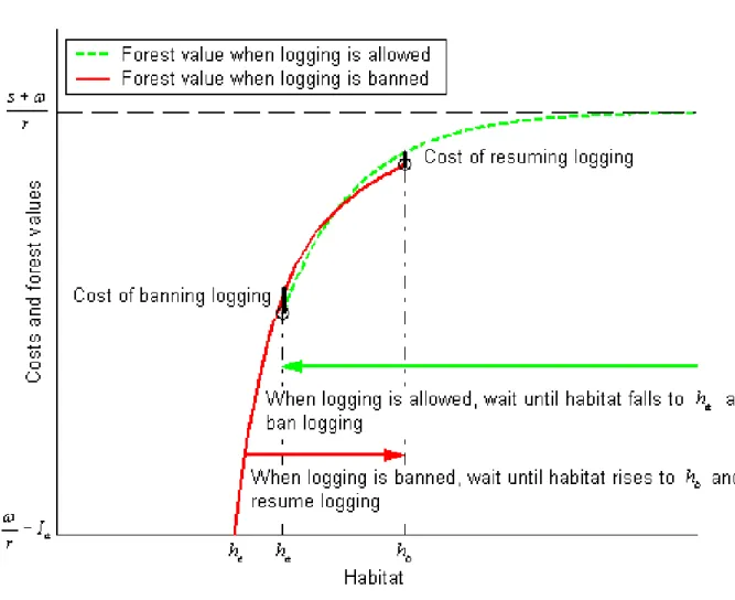
(20) reintroducing logging if and when the ban is lifted. Thus the con…guration involving a possible ban on logging is more likely to arise the higher s and the lower !. Meanwhile, since extinction is possible, the contribution of caribou to cumulated expected value is strictly lower than. s r. while logging’s contribution may reach. ! r. if no ban. is ever introduced. However, the possibility to manage logging regimes and bans reduces the opportunity cost of a logging ban to less than. ! r. so that s should not necessarily. exceed ! in order the con…guration involving a possible ban on logging to arise. In our application to Rangifer tarandus caribous though, it is found numerically that s should exceed ! by more than 10% in order that con…guration to arise. The optimal decision rule is illustrated in Figure 1. If the species is in existence and logging is allowed, which is compatible with past applications of the optimal rule if h 2 [ha ; +1[, then logging should continue as long as the current habitat level, driven by (1) for i = a, remains above ha (upper arrow); the forest value is then Va (h). As soon as h falls down to ha , logging is banned at cost Ib and the forest value becomes Vb (h); habitat is then driven by (1) with i = b. Logging remains banned as long as the current habitat level is between he and hb (lower arrow). Although this ban is favorable to habitat recovery, extinction may occur as it remains possible for h to fall to he . If and when this happens, logging is resumed forever at cost Ia yielding a forest value. ! ; r. the net present value of a forest reaching caribou extinction during a. logging ban is thus Vb (he ) =. ! r. Ia as the cost of allowing logging must be incurred prior. to drawing bene…ts. Although habitat may recover and reach levels above he later on, extinction is irreversible so that forest value remains at. ! r. even at values of h exceeding. he once extinction has occurred4 . However, when logging is banned, the probability that the habitat level remains above he is higher than when logging is allowed, as h is driven towards. b. >. a. by the non stochastic component of (1) for i = b. During a ban, habitat. is likely to increase and so does Vb (h) until hb is reached. At that habitat level the risk of extinction no longer justi…es foregoing logging income and the option to end the ban If !r Ia < 0, in violation of Assumption 2, logging is never resumed (in fact it was never worth undertaking) and the forest has no value anymore after extinction. 4. 17.

(21) Figure 1: The decision rule and the value functions at alternative habitat levels when logging is allowed or prohibited. 18.

(22) is exercised. The introduction of a logging ban reduces the short-run risk of extinction. Just before the ban, the short-run risk of extinction is Ra (ha ); once logging is banned, the risk becomes Rb (ha ). Intuition suggests, and our numerical results con…rm, that ha increases with the existence value of caribous: when s is higher, logging is interrupted farther above the extinction level because the cost of extinction, which is the expected value of being deprived from caribous, is higher. Raising ha , by reducing the probability of extinction, reduces that cost. For the opposite reason, a rise in the cost of interrupting logging justi…es accepting a higher risk of extinction in the hope of avoiding or postponing that cost: ha diminishes when Ib increases. A rise in the cost of resuming has the same e¤ect, although weakened because that cost is incurred in the future. As indicated in Proposition 2:2 though, adjustments to changes in s, Ia or Ib can reach a limit: for any given value of Ia and Ib , there is a value of s, s, below which ha no longer exists. 3.4. The mean durations of the forestry regimes. Besides the direct costs Ia and Ib of interrupting or resuming logging and besides e¤ects on timber revenues, switching between alternative forestry regimes implies various social disruptions that are likely to be more acute, the more frequent the switches. Longer logging periods are probably better than short logging spikes for forest communities. In any case the expected duration of logging regimes and bans is a crucial characteristic of the optimal rule. The mean duration of a ban Teb is the expected time for h to hit. either hb or he when its current level is ha and it follows the di¤usion process (1), with i = b. Similarly, the expected duration of a logging period Tea is the expected time for the di¤usion process (1) to reach ha for the …rst time when its current level is hb and when i = a. Proposition 3 gives explicit expressions for the mean durations of each forestry regime. In order to establish that proposition, we use the following lemma adapted from Karlin and Taylor (1981). Let Tih;h (h) denote the date at which the di¤usion process (1) hits either h or h (h < h) for the …rst time given that its current level. 19.

(23) h 2 [h; h]; that is Tih;h (h) = min(Tih (h); Tih (h)). Lemma 2 The expected time for the regular di¤usion process (1) to reach either h or h given its value h 2 [h; h] at time zero is ETih;h (h) ( Z h Z h;h h;h Si (h) Si ( ) mi ( )d + 1 Pi (h) = 2 Pi (h) h. (Si ( ). Si (h)) mi ( )d. h. 2 S 0 (h) i i. Rh h. ). denotes the speed density function of process (1) and Pih;h (h) =. 1. where mi (h) = R h 2i (x i )2 e i dx h. h. e. i 2 (x i. i). 1. 2. is the probability for the process to reach h before. dx. h given its current level h. Proof. Let Tei (h) denote ETih;h (h). For h 2]h; h[ and for a su¢ ciently small time. interval dt, the di¤usion process (1) does not hit either h or h during a time interval dt over which h evolves to h + dh; that is Tei (h) = dt + Tei (h + dh). By ap-. plying Ito’s lemma to Tei (h), one shows that Tei (h) satis…es the di¤erential equation 2 i. T 00 (h) + i ( i h) Ti0 (h) + 1 = 0. To solve that equation, use the canonical represen2 i tation of the di¤erential in…nitesimal operator associated with the di¤usion process (1), h i 2 Rh dTi (h) d that is express i Ti00 (h) + i ( i h) Ti0 (h) as 12 dM with M (h) = mi ( )d i dS (h) i i 2 where mi (h) = 2 S10 (h) is the speed density function of the di¤usion process (1)5 . To i. i. establish this canonical representation, note that the scale function Si (h) of (1) sat00. S (h). is…es by de…nition i ( 2i=2h) = Si0 (h) . As the di¤erential equation at hand becomes i i h i dTi (h) 1 d = 1, it can be integrated successively. Clearly, two boundary condi2 dMi dSi (h). tions apply: Tei (h) = Tei (h) = 0. For more details, see Karlin and Taylor (1981 p: 197). R h 2i (x i )2 To compute mi (h) = 2 S10 (h) , note that Si (h) = he e i dx by Proposition 1, so i. that mi (h) =. 1. 2 i. e. i 2 (h i. i. i). 2. .. Proposition 3 follows from Lemma 2 by noting that Tea = ETaha ;+1 (hb ), Teb = ETbhe ;hb (ha ),. and that limh!+1 Paha ;h (hb ) = 0.. Proposition 3 Suppose that the species is not extinct and that ha exists. 5. The name of ’speed density’can be justi…ed as follows: for a natural and regular di¤usion process xt , "2 m(x) is of the same order as the expected time for the process to leave the interval ]x "; x + "[ where x is its state at time zero and " is positive and small relative to x.. 20.

(24) 1. The mean duration of a logging ban is Teb = 2 Pbhe ;hb (ha ) + 1. Z. hb. (Sb (hb ). ha. Pbhe ;hb (ha ). Z. Sb ( )) mb ( )d. ha. (Sb ( ). Sb (he )) mb ( ) d. he. 2. The mean duration of a logging period is Tea = 2. Z. hb. (Sa ( ). Sa (ha )) ma ( )d. ha. 4. Optimal forest management rule and sensitivity analysis 4.1. Estimation of the stochastic process governing caribou habitat. The herd of Central Labrador’s Rangifer tarandus Caribous, also known as Red Wine Mountains caribous, occupies an area of about two million hectares corresponding approximately to Labrador’s Forest District 19A, near Goose Bay, Newfoundland and Labrador, Canada. Although non-subsistence hunting was prohibited in 1972, its population declined signi…cantly from over 700 animals in the 1980’s to 151 by 1997 (Schaefer et al. 2001). The species was listed as threatened in 2002 and subsistence hunting was banned. With little other threats to their livelihood, it is believed that the caribous hold a good prospect for survival. The main risk that they face is encroachments by human activities and development on their habitat. Caribou habitat typically consists of contiguous areas of old forest with minimal human disturbance (Schmelzer, 2004). The town Happy Valley-Goose Bay has about 8; 000 aboriginal and non-aboriginal inhabitants. The nearby Innu community of Sheshatshiu has a population of about 1; 600 people and lives on Forest District 19A. In the past, the Canadian Forces Base in Goose Bay was a major source of local employment and socio-economic development although bene…ts to the Innu Nation remain a contentious issue. Currently, the base operates on a reduced scale. Caribou may not be as critical to the Innu community as they once were but they are still central to their culture and highly valued. Labrador’s Forest District 19A has never been commercially exploited in any signi…cant way. It is 21.

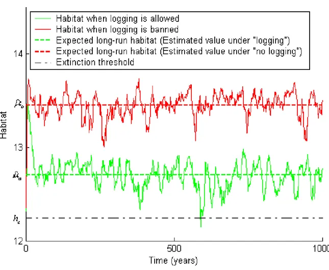
(25) currently proposed to substantially develop logging in the region, a project jointly conducted by the Innu Nation government and the Labrador Department of Forest Resources and Agrifoods. The main impact on the caribou herd would be habitat destruction or fragmentation. Using a landscape level disturbance simulation model, the Spatially Explicit Landscape Event Simulator (SELES) due to Fall and Fall (2001), we generated caribou habitat series simulating forest management with logging and without logging alternatively. The SELES model is a grid-based, spatiotemporal model, that incorporates both landscape characteristics, plausible disturbances such as wild …res or infestations, and forest management practices, to generate indicators of forest structure as it evolves over time. For the purpose of this application, the logging regime is based on the rate of harvest described in the forest management planning documents (Forsyth et al., 2003) for the period 2003. 2023. The logging rate is assumed constant at 62 000 m3 per year, which. corresponds to the maximum sustainable yield. Being the main natural perturbation a¤ecting caribou habitat, wild …res are the sole source of stochastic disturbance explicitly introduced in the model. Based on the size and frequency of …res in the past thirty …ve years (Morgan et al., 2008), the model is set to assume a …re rotation6 of 343 years. Considering the slow rate of growth of the boreal forest (Fahrig 2001), we generate Monte-Carlo habitat series that extend over one thousand years on ten-year intervals, starting with current period 2003. 2008 conditions. One such series for each forestry. regime is illustrated in Figure 2. One notes that extinction occurs after about six hundred years in the sample curve with logging. No such event happens in the case where logging is prohibited; however, while less probable in the short run, extinction occurs with probability one over an in…nite period. The analysis of the habitat series generated by SELES indicates that their autoregressive correlation coe¢ cients are decreasing while their partial autoregressive correlation coe¢ cients are negligible except for the …rst-order coe¢ cient. Consequently, both the habitat series with logging (i = a) and without logging (i = b) can be assumed to be 6. The …re rotation is the time required to burn a surface equivalent to the reference area.. 22.

(26) Figure 2: Two realizations of caribou habitat from the SELES landscape model (logging and "no logging" regimes). 23.

(27) Gaussian autoregressive processes of order 1 (AR1). We write them as discrete versions of (1):. with. i. > 0,. i. =e. i. hit =. i (1. < 1,. 2 i. =. i). +. 21 e i 2. i ht 1 2 i. i. +. i "it ;. (13). i = a; b. , and where "it is a standardized Gaussian. white noise (for more details, see Gouriéroux and Jasiak, 2001, chapter 11). Box-Pierce and Breusch-Godfrey Lagrange multiplier tests validate this representation as they exhibit uncorrelated error terms. The sample was used to estimate (13). The Maximum Likelihood estimators are7 : Forestry Regime: Estimated values: Long-run expected habitat : bi Speed of reversion (per decade): bi Variance (per decade): bi. logging allowed: i = a mean st. dev. 12:7034 0:00497 0:0575 0:011 0:0028. logging banned: i = b mean st. dev. 13:4504 0:00513 0:0532 0:0106 0:0028. According to the estimated parameters, logging a¤ects the long-run level of habitat. (ca < bb ) as expected but has little e¤ect on the speed of reversion and on the volatil-. ity. Introducing logging causes the long-run level of caribou habitat to decrease from 694 110 ha to 328 860 ha (from 62% to 29% of the forest area), a drop of more than. 50%. As discussed in Section 2, a landscape becomes inadequate as caribou habitat when less than 30% of old growth habitat is intact. In this context old growth habitat must be interpreted as the expected long-run habitat level when logging is banned. Then the level of habitat corresponding to caribou’s extinction can be estimated to be around 30% of e. b. or 208 230 hectares, which is signi…cantly lower than the long-run habitat. level when logging is taking place; in logarithm, this translates to he = 12:2464, or 18% of the forest area. 7. 100 be the number of observations. For i = a; b, bi = PT h 2 2 it t=1 (hit hiT )(hi;t 1 hiT ) 2 bi log ; and bi = where hiT = t=1 , bi 2 = PT 2 c b T 1 e 2 i i t=1 (hit hiT ) b b "2it = hit hiT e i hi;t 1 hiT . Let T PT. =. 24. hiT ,. PT. "2it t=1 b T. bi. =. , and.

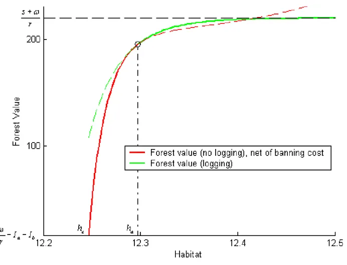
(28) 4.2. Application of the real option model. Assuming constant timber prices, the ‡ow of logging revenues is constant. We set ! to unity, so that all monetary values in the model have to be multiplied by the actual logging revenue ‡ow to give nominal dollar …gures. We use a discount rate of 5%. As it is di¢ cult to get accurate estimations of the costs to ban and to resume logging, we assume Ia and Ib to represent alternative percentages of logging revenues and conduct an analysis of the decision rule’s sensitivity to that percentage. Unless otherwise mentioned, Ia and Ib are both set to 10% of an hypothetical perpetuity. ! r. from logging revenues,. that is Ia = Ib = 2 for ! = 1 and r = 5%. The existence value of the caribous is a very important and controversial issue. While some Innus consider the caribous to be priceless and their existence beyond evaluation, some also consider that the very existence of the Innus as a distinct culture is compromised by economic hardship. Logging and learning how to control that activity might be one way toward survival and adaptation. While these views appear in contradiction with each other, the model clari…es at least two points about the relative values of ! and s. The …rst one is that, by Proposition 1, there exists some upper threshold hb above which logging should be allowed however high the existence value of the species. The second point is that, by Proposition 2, it is possible for the existence value of the caribous to be low enough with respect to logging revenues for a logging ban never to be optimal. This relative value depends on all other parameters and can be computed; in the current application, s must be higher than ! by more than 10% if logging is ever to be banned. Consequently we describe the optimal decision rule for a range of s=! values strictly above unity; as a base case and unless otherwise mentioned, s equals 10 times !. The forest value functions Vb and Va are computed numerically as solutions to (3) (6) and (9). (12) respectively by adapting the box method described in Zwillinger. (1998). Figure 3 represents the forest value function Va (h) for values of h above ha . The threshold ha applies when it is crossed from the right to the left; it is equal to 12:2972. 25.

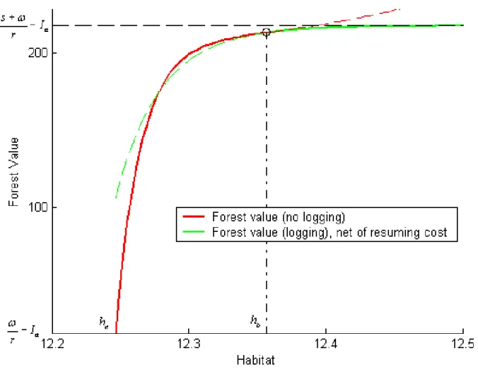
(29) which implies that logging is to be interrupted if habitat gets down to 219 082 hectares, which is only 5% above the extinction level and dangerously close to it. The …gure also illustrates the value-matching and smooth-pasting conditions that link Va (h) and Vb (h) at ha . Since the value matching condition is Va (ha ) = Vb (ha ). Ib and the relevant. function to the left of ha is Vb (h), the plain curve to the left of ha represents the forest value function net of the cost of banning logging, Vb (h). Ib .. Figure 3: Forest value and habitat threshold during a logging regime. Once logging has been banned, the forest value function is Vb (h) and this situation continues as long as habitat does not cross, from the right, the extinction threshold he or, from the left, the threshold hb at which logging should be resumed. That threshold 26.

(30) is equal to 12:3567 or 232 513 hectares, which amounts to 12% more than the extinction threshold. When hb is reached, logging is resumed at cost Ia and the forest value function becomes Va (h) as long as habitat remains above ha . Figure 4 illustrates the value-matching and smooth-pasting conditions between Vb (h) and Va (h). Ia at hb .. Figure 4: Forest value and habitat threshold during a logging ban. As implied by Proposition 2:3, even if Assumptions 2 and 3 are satis…ed, there may not exist any value of h compatible with current caribou existence at which a ban on logging is optimal. However, while ha may not exist, hb always does. Both thresholds, as well as the short-run extinction risks Ra (ha ) and Rb (ha ), vary with the existence value of the caribous as represented by s. In the base case, the short-run extinction risk 27.

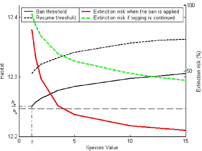
(31) decreases from approximately Ra (ha ) = 50% to Rb (ha ) = 10% when logging is banned at h = ha . This is a reduction of about 80%. Figure 5 illustrates the sensitivity to s of the thresholds ha and hb , and of the shortrun extinction risks at the time logging is interrupted. The extinction risk curves are decreasing as implied by Proposition 1. The curves describing ha and hb as functions of s are rising. That is to say, at higher values of s, a logging regime is interrupted earlier (ha is higher) and a ban on logging is ended later (hb is higher), than at low values of s. When s is low, habitat is allowed to come closer to the extinction level before logging is banned; however the banning threshold is strictly higher than he . As implied by Proposition 2:3, ha does not exist for values of s below s; this critical species value turns out to be 10% higher than ! and is associated with a threshold ha which exceeds he by only 0:5%; indeed the risk of extinction is allowed to become as high as 82% before logging is interrupted. Figure 6 applies Proposition 3 to compare the mean duration of a ban with the mean duration of a logging regime at various levels of s. In the base case, when s = 10!, the former is about 8 years while the latter is around 86 years; furthermore this di¤erence in favor of logging increases as s increases. Meanwhile, as the …gure also indicates, the relative change in extinction risk when a ban is introduced is quite drastic, at about 80% in the base case, and rising with s. This means that a policy optimally designed to protect the caribous by banning logging temporarily is quite attractive as it does not require long banning periods while it drastically reduces the risk of extinction8 . The longer expected duration of logging regimes stems from the fact that such regimes apply at higher habitat values: h 2 [ha ; +1[. Since. a. 2 [ha ; +1[, this means that. the interval includes values where the deterministic component of the habitat’s motion is zero or small; at higher values, the motion may be fast but no regime change may occur. Thus h tends to stay for extended periods in that regime. In contrast, bans involve values of h in [he ; hb ]; as hb turns out to be lower than. b,. this means that bans. 8 This property emerges from the numerical analysis and appears to be robust to the range of parameters that we have considered.. 28.

(32) Figure 5: Habitat triggers (left-hand scale) and short-run extinction risk (right-hand scale) according to species value. 29.

(33) Figure 6: Mean duration of forestry regimes (left-hand scale) and impact of a ban on short-run extinction risk (right-hand scale) according to species value. 30.

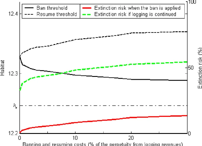
(34) are associated with relatively fast changes in habitat, so that they do not last on average as long as logging regimes do. It is also surprising at …rst to see that the mean duration of logging regimes increases with s. Indeed, since ha increases with s it takes less time, the higher s, for habitat to reach ha from any level h > ha ; this factor reduces the expected duration of logging at higher values of s: However, since hb also increases with s, logging is introduced at higher levels of h, the higher s; this means that it takes longer for h to reach from hb any given level below hb ; this factor increases the expected duration. Furthermore hb being closer to. b,. the higher s, logging starts in a zone where h is not moving fast, and more. so, the higher s. Together these last two factors dominate the …rst one and explain why the mean duration of logging regimes increases with the existence value of the species. The next two …gures illustrate the impact of the discount rate. Figure 7 demonstrates its impact on ha , hb , and on the short-run extinction risk at the time logging is interrupted. Higher discount rates require logging to be resumed earlier and banning to occur later as both ha and hb decrease when the discount rate increases. In both cases, a higher discount rate reduces the weight assigned to future extinction so that it promotes risk taking. Figure 8 illustrates the sensitivity to the discount rate of the expected logging and ban durations. The expected duration of a logging period decreases as ha and hb become closer to each other as a result of the increase in r; similarly the expected duration of a ban decreases as hb becomes closer to he . The costs of interrupting or reintroducing logging are other factors a¤ecting thresholds and optimal short-run risks of extinction. Figure 9 depicts how the habitat thresholds and extinction risks hb and ha vary according to Ia and Ib . When Ib increases, the decision to ban is delayed so that ha becomes closer to the extinction level he . Similarly, when Ia increases, the decision to resume logging is delayed and hb increases. The costs Ia or Ib are incurred at the time the change in logging regime is implemented and their e¤ect is intuitively obvious. However another, indirect, cost of a change in logging regime is the cost that will be incurred in the future when a new regime change is called 31.

(35) Figure 7: Habitat thresholds (left-hand scale) and short-run extinction risk (right-hand scale) according to the discount rate. 32.

(36) Figure 8: Mean duration of each forestry regime according to discount rate. 33.

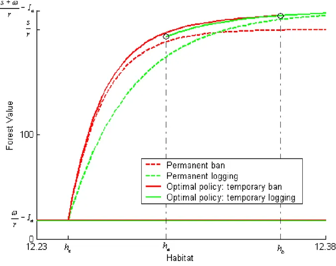
(37) for. If the cost of reverting in the future to the logging regime being abandoned is high, the decision will be postponed. This means, e.g., that an increase in Ib not only reduces ha but also raises hb . The …gure does not separate such secondary e¤ect from the direct e¤ect as Ia and Ib are taken to be equal and vary together as a percentage of !=r.. Figure 9: Habitat triggers (left-hand scale) and short-run extinction risk (right-hand scale) according to the costs of interrupting or resuming logging. Finally, Figure 10 illustrates the extent to which adopting the optimal management rule described in this paper increases forest value relative to the value achieved under two alternative, sub-optimal, policies. The …rst alternative consists in allowing logging forever while the second alternative consists in banning logging forever as long as the species is in existence, and introduce logging if it becomes extinct. In order the alter34.

(38) native value curves to be comparable, we assume that the initial situation is such that no logging is going on. Introducing logging consequently requires the initial outlet Ia whether this is a permanent change or a temporary one. On the contrary, the permanent ban policy does not involve any expenditure. Under the optimal policy, the initial logging ban continues until either habitat falls to the extinction threshold (then logging is resumed forever), or habitat increases to hb (then logging is allowed and goes on as long as habitat remains above ha ). The continuous curves represent the corresponding value function. Allowing logging forever amounts to giving up the option to protect the species; this option is less valuable when habitat is abundant and the species is not immediately threatened. The forest value function corresponding to that policy is V~a (h), de…ned by (8) and characterized in Proposition 2:2. It is lower than the optimum value function and approaches it when h tends to in…nity. At …nite habitat values, the di¤erence is strict; for example, the optimum policy increases forest value by 11% over the permanent logging policy when h = ha . The policy of banning logging until extinction is a lesser mistake when habitat is low because the optimal policy then requests to prohibit logging anyway, at least temporarily. In fact, when h tends toward the extinction threshold, the value achieved by a permanent ban tends toward that achieved by the optimal policy. This is because, in case of extinction, logging is introduced or reintroduced in both cases. The forest value function arising from a permanent ban policy is: "Z he Tb (h) he ! ~ Vb (h) = E se r d + e rTb (h) r 0. Ia. #. jh0 = h ; 8h 2 [he ; +1[. One can show that it must solve 2 b. 2. V~b00 (h) +. b. (. b. h) V~b0 (h). rV~b (h) + s = 0; 8h 2]he ; +1[. with the two boundary conditions: ! V~b (he ) = r 35. Ia.

(39) s lim V~b (h) = h!+1 r When h = hb , the optimal policy yields 7% more than a permanent ban; when h tends toward in…nity, it yields 9% more.. Figure 10: Comparing forest values under the optimal policy, under a permanent ban, and under permanent logging. 5. Conclusion The real options model that we have presented applies when human activity may a¤ect a species or a natural site adversely. It optimizes the trade-o¤ between the bene…ts associated with this activity and the risks involved for the natural environment. Partial or total irreversibility is present not only as extinction is …nal but also as policy changes 36.

(40) are costly to introduce and to undo. Uncertainty a¤ects the evolution of the species or site. In the empirical application that we have presented, the habitat of the species is a stochastic variable which is currently observable but whose future level is unknown. The objective of the decision maker is to maximize expected future bene…ts from the forest, that is to say bene…ts derived from the existence of the endangered species and bene…ts derived from timber exploitation. The sole instrument to achieve this objective is the discretion to ban logging if habitat becomes dangerously low, and to resume logging if habitat recovers su¢ ciently. Besides the obvious e¤ect on wood harvest, such changes in the logging regime a¤ect the stochastic process governing habitat. In the empirical application presented in the paper the stochastic process was estimated by Monte Carlo methods for each regime. Given the uncertainty surrounding the future, the decisions to authorize or to ban logging are not speci…ed in advance; what is speci…ed by solving the optimization problem is a rule to be followed in the future and according to which the current logging regime is maintained or interrupted depending on the current habitat level. As usual in real options models, the optimal rule takes advantage of uncertainty in such a way as to increase exposure to favorable outcomes (when the habitat grows more than expected), while seeking protection from unfavorable outcomes (low habitat levels). Interrupting logging when habitat is dangerously low does not guarantee that extinction will not occur but reduces its probability, thus providing (partial) protection against that unfavorable outcome. In that respect the model just presented is a rigorous application of the precautionary principle. It does not rule out risk taking, but agrees with the conventional wisdom that decisions should bend the distribution of risk a community is exposed to in such a way as to reduce the probability of irreversible catastrophes. Whether the current regime allows or prohibits logging, there is a well de…ned probability of extinction over any …nite horizon, and that probability is higher, the closer habitat is to the extinction level. The decision rule established in the paper optimizes the trade-o¤ between the risk of extinction and the bene…ts derived from logging. We 37.

(41) have described it in terms of the habitat levels that trigger logging bans or resumptions, but also in terms of the risks of extinction, and in terms of the value derived by the community from the forest. We have also compared the forest value achieved by using the optimal policy to the values implied by less sophisticated policies; the gain is of the order of 10% at empirically relevant habitat levels. Such magnitudes provide alternative, perhaps more intuitive, descriptions of the optimal policy, as also do the mean durations of each regime. Whatever the way the optimal policy is examined, it appears to provide an attractive and simple solution to the problem of protecting a species while not giving up other bene…ts altogether. The existence value of the endangered species is central to the model and determines the risk of extinction implied by the optimum rule. While the existence value is always di¢ cult to estimate and controversial, to the point that stakeholders frequently deny that it is even amenable to any form of estimation, the same actors are often willing to consider risks of extinction and to evaluate the e¤ect of policy decisions on such risks. By making explicit the relationship between existence value and the willingness to increase the extinction risk under the optimal policy, our model can also be viewed, and used, as a way to infer a species valuation from the willingness to take risks with respect to its survival.. 38.

(42) References Allee, W.C., A.E. Emerson, O. Park, T. Park, K.P. Schmidt (1949) Principles of animal ecology, Saunders, Philadelphia. Andrén, H. (1994) “E¤ects of habitat fragmentation on birds and mammals in landscapes with di¤erent proportions of suitable habitat: a review”Oikos 71(3), 335-366. Brown, J.H. and A. Kodric-Brown (1977) “Turnover Rates in Insular Biogeography: E¤ect of Immigration on Extinction”Ecology (58), 445-49. Conrad, J. (2000) “Wilderness: options to preserve, extract, or develop” Resource and Energy Economics (22), 205-19. Dixit, A.K. (1993) The Art of Smooth Pasting, Harwood academic publishers. London, Paris. Dixit, A.K., and R.S. Pindyck (1994) Investment Under Uncertainty, Princeton, NJ, Princeton University Press. Fahrig, L. (2001) “How much habitat is enough?” Biological Conservation 100(1), 6574. Fahrig, L. (2002) “E¤ect of habitat fragmentation on the extinction threshold: A synthesis”Ecological Applications 12(2), 346-353. Fall, A. and J. Fall (2001) “A domain-speci…c language for models of landscape dynamics”Ecological Modelling (141),1-18. Forsyth, J., L. Innes, K. Deering, and L. Moores (2003) Forest Ecosystem Strategy Plan for Forest Management District 19 Labrador/Nitassinan. Innu Nation and Labrador Department of Forest Resources and Agrifoods. Insley, M. (2002) “A Real Options Approach to the Valuation of a Forestry Investment” Journal of Environmental Economics and Management (44), 471-92. Karlin, S. and H. M. Taylor (1981) A Second Course in Stochastic Processes, Academic Press. Kassar, I. and P. Lasserre (2004) “Species preservation and biodiversity value: a real options approach” Journal of Environmental Economics and Management 48(2), 85779. 39.

(43) Labrador Department of Forest Resources and Agrifoods (2003) Five Year Operating Plan for Forest Management District 19A. Goose Bay, Labrador, NL. Morgan D., S., S. Ben Abdallah, and P. Lasserre (2008) “A Real Options approach to forest management decision making to protect caribou under the threat of extinction” Ecology and Society, 13(1). Pindyck, R. (2000) “Irreversibilities and the timing of environmental policy” Resource and Energy Economics, (22), 233-59. Saphores, J.-D. (2003) “Harvesting a renewable resource under uncertainty”Journal of Economic Dynamics & Control (28), 509-29. Saphores, J.-D. and J. Shogren (2005) “Managing Exotic Pests under Uncertainty: Optimal Control Actions and Bioeconomic Investigations” Ecological Economics 52(3), 327-39. Schaefer, J. A., A. M. Vietch, F. H. Harrington, W. K. Brown, J. B. Theberge, and S. N. Luttich (2001) “Fuzzy structure and spatial dynamics of a declining woodland caribou population”Oecologia (126), 507-14. Schmelzer, I., J. Brazil, T. Chubbs, S. French, B. Hearn, R. Je¤ery, A. McNeill, R. Nuna, R. Otto, F. Phillips, G. Mitchell, G. Pittman, N. Simon, and G. Yetman (2004) Recovery strategy for three woodland caribou herds (rangifer tarandus caribou; boreal population) in labrador Department of Environment and Conservation, Government of Newfoundland and Labrador, Corner Brook, NFLD, Canada. Zwillinger, D. (1998) Handbook of Di¤erential Equations, MA Academic Press.. 40.

(44)