Connolly Pray : Département des sciences économiques, ESG UQAM, C.P. 8888, Succ. Centre-ville, Montréal, QC, Canada H3C 3P8 ; tél. : 514 987-3000 ext. 0277; fax : 514 987-8494
connolly-pray.marie@uqam.ca
Funding from SSHRC and FQRSC is greatly acknowledged. I would like to thank Alan Krueger for making the data available and the project possible and Rod Hill for helpful comments. Yann Fortin provided excellent research assistance. All remaining errors are my own.
Cahier de recherche/Working Paper 11-16
Some Like It Mild and Not Too Wet : The Influence of Weather on
Subjective Well-Being
Marie Connolly Pray
Abstract:
More and more economists and politicians are advocating the use of comprehensive measures of well-being, on top of the usual national accounting measures, to assess the welfare of populations. Researchers using subjective well-being data should be aware of the potential biasing effects of the weather on their estimates. In this paper, I investigate the responsiveness of well-being to climate and transitory weather conditions by analyzing subjective well-being data collected in the Princeton Affect and Time Survey. I study general satisfaction questions about life in general, life at home, health and one’s job, as well as questions concerning feelings intensities during specific episodes. I find that women are much more responsive than men to the weather, and that life satisfaction decreases with the amount of rain on the day of the interview. Low temperatures increase happiness and reduce tiredness and stress, raising net affect, and high temperatures reduce happiness, consistent with the fact that the surveys was conducted in the summer. I conclude by suggesting methods to reduce the possible biases.
Keywords: Subjective well-being, life satisfaction, happiness, weather, temperature,
precipitation
1
Introduction
Economists are increasingly interested in subjective well-being assessments. While psychologists have for many years studied happiness—its definition, its causes, its correlates, its social context and more1—it is rather recently that economists have departed from the sacrosanct focus on output growth to advocate for a more inclusive conception of well-being. As Frey and Stutzer summarized in their 2002 survey of the literature on happiness research: “It follows that economics is—or should be—about individual happiness (Frey and Stutzer, 2002, p. 402).” In 2008, French President Nicolas Sarkozy commissioned a team of experts led by Nobel prize winners Joseph Stiglitz and Amartya Sen to identify the limits of GDP as a measure of economic performance and social progress. In their final report, they note that “[m]easures of both objective and subjective well-being provide key information about people’s quality of life,” and follow by recommending that “[s]tatistical offices should incorporate questions to capture people’s life evaluations, hedonic experiences and priorities in their own survey (Stiglitz, Sen and Fitoussi, 2009, p. 16).” One example of recent efforts to report on quality of life is the OECD’s “Better Life Index,” which incorporates 11 measures including life satisfaction.2 The British magazine The Economist has surfed the trend and more than once proposed online debates about happiness on its website3 or published articles on the issue.
In opposition to objective measures of well-being such as income, life expectancy, housing conditions and other observable factors, subjective measures rely on people’s own evaluations of their condition. It is generally accepted that there are many indicators of subjective well-being (SWB), each measuring a specific component that contributes to SWB in its own way (Krueger, 2009; Bok, 2010; Helliwell and Barrington-Leigh, 2010). Satisfaction with life is one of the more common concepts and asks that people evaluate their lives “as a whole.” This will usually involve a cognitive process using a reflection and a judgment of their broad and continuing life circumstances. At the other end of the spectrum, positive and negative emotions reflect experienced happiness and relate to an individual’s affective state at a given moment. Such positive and negative affects are effectively measured as part of time-use surveys, or what Krueger et al. (2009) refer to as their approach of National Time Accounting4 (see also Helliwell and Barrington-Leigh, 2010 and Diener et al., 2009). The reliability of subjective well-being measures is a serious concern and as such
1The major works that come to mind are Kahneman, Diener and Schwarz (1999), Argyle (2001) and Strack,
Argyle and Schwarz (1991).
2See OECD (2011) and http://www.oecdbetterlifeindex.org/.
3See http://www.economist.com/debate/overview/204/Happiness for the most recent debate.
4In Krueger et al.’s own words, “National Time Accounting is a set of methods for measuring, categorizing,
comparing, and analyzing the way people spend their time, across countries, over historical time, or between groups of people within a country at a given time. . . . The methods we propose provide a means for evaluating different uses of time based on the population’s own evaluations of their emotional experiences, what we call evaluated time use, which can be used to develop a system of national time accounts.” (Krueger et al., 2009, p. 11)
has been extensively tested in numerous studies.5 Bok (2010) concludes that “[a]ll in all . . . careful researchers seem to measure happiness or dissatisfaction with enough accuracy to make the results useful for policy-makers.” (p. 39) However he goes on to say that “[i]t is true that a variety of transitory influences can affect people’s judgments about how happy or satisfied they are. Most of the time, however, these distortions are sufficiently random to cancel themselves out in surveys involving substantial numbers of people.” (p. 39)
One such transitory influence is the weather. Weather conditions affect mood and prosocial behavior. Cunningham (1979) found markedly increased tipping to restaurant waiters on sunny days and attributes the behavior to the impact of sunshine on mood.6 Smith (1979) documented the seasonal pattern of happiness and affect—but found no such pattern in life satisfaction. The existence of Seasonal Affective Disorder (SAD) as a mental health condition has long been rec-ognized, with winter months associated with the highest level of seasonal depression (Oren and Rosenthal, 1992). Keller et al. (2005) and Denissen et al. (2008) both provide more recent examples of psychological studies linking mood to weather conditions. Economists have studied the effect of sunshine on stock market returns, suggesting that investors’ good mood on sunny days influences their cognitive processes and trading decisions (Saunders, 1993; Hirshleifer and Shumway, 2003; Dowling and Lucey, 2005; Goetzmann and Zhu, 2003). While the link between meteorological conditions and affect is intuitive, the association with life satisfaction is less straightforward. If satisfaction with life is supposed to be an assessment of how good one’s life is in general, should it vary depending on whether the sun is shining or not on the day the question is asked? Schwarz and Clore (1983) found that people reported significantly higher general happiness, life satisfac-tion, and content with current life7 on sunny vs. rainy days. However, when first primed about the weather, rainy-day subjects were better able to attribute the source of their sour mood to the weather conditions and reported the same average life satisfaction as they would on sunny days. Simonsohn (2005) found that prospective college students who visit a school on a cloudy day are more likely to enroll in that school and that university admission officers place greater relative importance on academics when reviewing applications on cloudier days. He argued that cloudier weather makes people place more weight on academic factors, and less on social factors and enjoyment, while making decisions about which college to enroll in.
This brings up a question: Are people consistently affected by weather conditions when they respond to subjective well-being surveys? If yes, researchers studying well-being need to know
5See Bok (2010, chapter 2), Krueger et al. (2009) and Helliwell and Barrington-Leigh (2010) for literature surveys
on the reliability of SWB measures.
6Beliefs about weather, whether they turn out to be accurate, also seem to influence mood, as Rind (1996) and
Rind and Strohmetz (2001) found in their study of the impact of beliefs about weather on tipping.
about the effects of such conditions and, depending on the purpose of the study, may want to control for current weather or use priming to tease out the weather effect. Rehdanz and Maddison (2005) looked at the issue using country-level data and found that higher mean temperatures in the summer months decrease happiness, while higher mean temperatures in the winter months increase it. Barrington-Leigh (2008) investigated the question using Canadian data on satisfaction with life. He found that after controlling for local climate expectations, recent cloud cover was significantly and negatively associated with satisfaction with life. Happiness8 did not appear to be correlated with his weather variables. He optimistically concludes that “[s]tatistical estimates which are not informed about the state of the weather produce the same inferences regarding the determinants of [satisfaction with life] as those which take weather’s influence into account.” (p. 26)
The present paper explores the relationship between weather, as characterized by temperature and precipitation variables, and subjective well-being in the United States, as measured by sat-isfaction with life and affective state. The influence of climate is also considered, although the exogeneity of climate is questionable. If people self-select into different climates based on the re-sponsiveness of their well-being to weather conditions, then the estimates of the impact of climate on SWB will be tainted by selection bias. There is some evidence that it may be the case (Rappa-port, 2007). A unique dataset from 2006, the Princeton Affect and Time Survey (PATS), is used in conjunction with weather records.
This paper starts in Section 2 with a presentation of the framework by which weather might correlate with subjective well-being and the models estimated in this study. The data used in the analysis are then presented in Section 3, and the findings in Section 4. Section 5 concludes.
2
Weather as a Process Influencing Well-Being and
Mod-els
Affect is the more direct and instantaneous facet of subjective well-being and is closely linked to mood and emotions. There can be positive affect (current mood: happy, interested) and negative affect (current mood: sad, depressed). Neuroscientists studying the brain have found that various neurotransmitters (dopamine, nor-adrenaline, endorphins) activate “pleasure centers” (Argyle and Martin, 1991), and have asked what triggers the release of those neurotransmitters.9 As mentioned
8Happiness was measured as the answer to the question “Presently, would you describe yourself as: very happy,
somewhat happy, somewhat unhappy, or very unhappy?”
9Argyle and Martin (1991) list many of the causes of joy, such as social contacts with friends, sexual activity,
in the introduction, Cunningham (1979) documented the impact of various weather measures on mood. The exact channel through which weather changes affect is unclear however: sunny days could directly raise the feeling of happiness, but sunny days could also lead people to spend more time outside in social leisure activities, which provide more happiness than work. This second channel is suggested by Connolly (2008) who found that men spent an extra half an hour working on rainy days compared to sunny days, and falls in the line of Krueger et al.’s (2009) work which seeks to relate “experienced happiness” (an aggregation of affect measures over a certain period of time like a day) to how people spend their time. Keller et al. (2005) documented the mitigating effect of time spent indoors (thus away from the elements) and of the season. They found that time spent outdoors increased the strength of the relationship between weather and mood, and that the effect was strongest in the spring, after a long period of deprivation from pleasant outdoors weather.
A second constituent of SWB is satisfaction. Faced with the complex task of evaluating their life satisfaction, people will often resort to heuristics or readily available information (Schwarz and Strack, 1991).10 The more global the concept to be evaluated (for example, when asked about life as a whole rather than satisfaction with job or health), the more likely the current affective state will be given informational value in shaping the judgment about well-being. Schwarz and Strack (1991) describe two processes by which mood states may impact satisfaction reports. First, the mood can increase the accessibility of “mood-congruent information from memory,” which means that one is more likely to recall positive events when in a happy mood, thus leading to a more positive evaluation of his or her life. Second, an individual can assume that his or her mood at the time of judgment is a “reasonable and parsimonious indicator” of general well-being. Whatever the psychological process, if weather shocks influence mood, then we can also expect them to have an impact on reports of life satisfaction (as is the case in Schwarz and Clore, 1983). After controlling for expected conditions, a given day’s temperature or precipitation level can reasonably be thought of as exogenous: an individual has no power over today’s cloudiness. On the other hand, in a model where households are mobile and can relocate, a locality’s climate is no longer exogenous. In fact, the decision to move to a certain area may be partly based on the climate. Rappaport (2007) observed that local population growth in the United States was highly correlated with warmer winter weather and cooler, less humid summer weather. He argued that people were moving to areas with better weather, due to an increasing valuation of this factor’s
10Schwarz and Strack (1991) note: “In reality, however, individuals rarely retrieve all information that may be
relevant to a judgment. Instead, they truncate the search process as soon as enough information has come to mind to form a judgment with sufficient subjective certainty [...] Hence, the judgment is based on the information that is most accessible at that point in time.” (p. 63)
contribution to their quality of life, which was, in turn, due to rising real incomes. This renders tenuous the interpretation of the link between climate and SWB as causal.11
Assuming that a given day’s weather is exogenous, the causal link between transitory weather (conditions the day of the interview) and well-being can plausibly be estimated from the following econometric model: SW Bijt= α + Wijt0 γ + N 0 ijtδ + X 0 ijtβ + φj + ψt+ uijt, (1)
where SW Bijt is the measure of interest for individual i in state j at time t, i.e. one of the four satisfaction variables (satisfaction with life, at home, with own health or at work), one the six affect variables (happy, interested, tired, stressed, sad, in pain) or one of the two measures constructed from the affect variables, the net affect and the U-index. (All these will be described in more detail in the Data section.) The vector W contains the weather variables: precipitation dummies for the interview day and the diary day, temperature dummies for the interview or diary day, and a variable counting the number of days since last dry day. The vector N contains normal precipitation and temperature, to control for climate. The controls (X ) include a quadratic in age and education, marital status, race and hispanic ethnicity dummies.12 State (φj) and time (ψt) fixed effects are included,13and u is the usual error term. The model will be estimated by ordinary least squares,14 with heteroskedasticity-robust standard errors clustered at the state or individual level15 to allow for intra-cluster correlations, and using the sampling weights provided with the data.
11This interpretation is made even more difficult by the potential focusing illusion that can come into play. For
example people generally think that they would be happier living in California when in fact studies have shown that they do not (Schkade and Kahneman, 1998).
12Household income is not used because too few respondents provided an answer. Coefficient estimates do not
change substantively but precision is lower.
13In regressions where an affect measure is explained, day of week and activity fixed effects are also included. 14To use a model better suited with the particular form of the data (answers are on a scale of 1 to 4 or 0 to 6),
ordered probits were used. However the results did not change significantly and so OLS results are presented for ease of interpretation.
15For satisfaction variables, there is only one observation per person so the clustering is at the state level,
whereas we observe affect for three different time-use episodes of a person’s day, which makes clustering possible at the individual level for affect variables.
3
Data
3.1
Princeton Affect and Time Survey
The affective data come from the Princeton Affect and Time Survey (PATS).16 The PATS was conducted by Gallup from May 4, 2006, to August 21, 2006, and collected information on time use and affect for 3,982 individuals as part of the Random Digit Sample, covering persons of age 15 and older living in the continental United States.17 The Random Digit Sample is nationally representative, and selected using an Equal Probability Selection Method. Each household was randomly assigned a day of the week, and once contacted, was asked about time use and affect for the previous day. The most recent birthday selection technique was used to designate a selected respondent among all household members 15 years of age or older. The survey was done over the telephone, using the same software used by the Bureau of Labor Statistics for data collection on the American Time Use Survey (ATUS) program. After the time-use module was collected, respondents were surveyed on their affect during three randomly selected 15-minute intervals of their day, excluding time spent sleeping and grooming. The selection of episodes in thus proportional to time spent in the episode, and was done without replacement. Survey weights were designed to maximize the representativeness of the data.18
During the Affect Module, respondents were asked to rate the intensity of six different feelings as experienced during each selected episode, using a scale of 0 to 6, where 0 marks a low intensity and 6 a high intensity of the feeling. The survey covered the following feelings: happiness, tiredness, stress, sadness, interest, and pain.19Table 1 contains descriptive statistics for the feelings questions, as well as tabulations by intensity of feeling. Two variables are constructed from the answers to the feelings questions: net affect and the U-index.20 Both give a different measure of well-being. The net affect is computed as follows:
Net affect = happy − mean(stressed, sad, pain) (2)
16The PATS data are publicly available online at http://www.krueger.princeton.edu/PrincetonAffectandTimeSurvey.php.
However note that the geographical identifier that allowed the weather variables to be added to the dataset is not publicly available due to confidentiality reasons.
17Another sample oversampled retirees; the retiree sample will not be used in this study. 18Summary statistics of the PATS sample are presented in the online appendix.
19The ordering of the emotions in the questionnaire was randomly varied. Krueger et al. (2009) found that when
asked about a negative feeling first, the responses about the following positive feelings were slightly lowered.
20See Kahneman and Krueger (2006) for a presentation and discussion of net affect and the U-index as
The U-index relates to the percentage of time spent in an unpleasant state (U is for ‘unpleasant’, and is computed according to the following equation:
U-index = (
1 if max(stressed, sad, in pain) > happy
0 otherwise (3)
The U-index is 1 when the most intense feeling is a negative one, and its use can be justified by the fact that most episodes of people’s days are pleasant, as can be seen in Table 1, and that any dominant negative emotion will, by its salience, reflect the way people judge their mood during that episode.
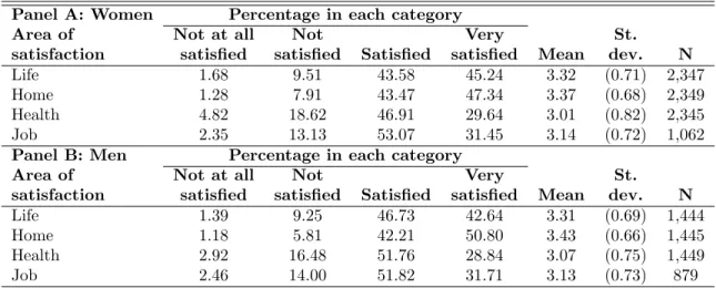
At the end of the Affect Module, a set of questions about general well-being was included. Respondents were to rate their satisfaction about their life overall, their life at home, their health, and their job if they had one, on a scale of 1 to 4, where 1 meant “Not at all satisfied,” 2 “Not satisfied,” 3 “Satisfied,” and 4 “Very satisfied.” As can be seen in Table 2, which contains sum-mary statistics and tabulations of the satisfaction questions, the majority of the people answered “Satisfied” or “Very satisfied” to these questions, with over 90% of the responses in these two categories for the life satisfaction and home satisfaction questions, and 74% and 85% for health and job satisfaction, respectively.
3.2
Weather Data
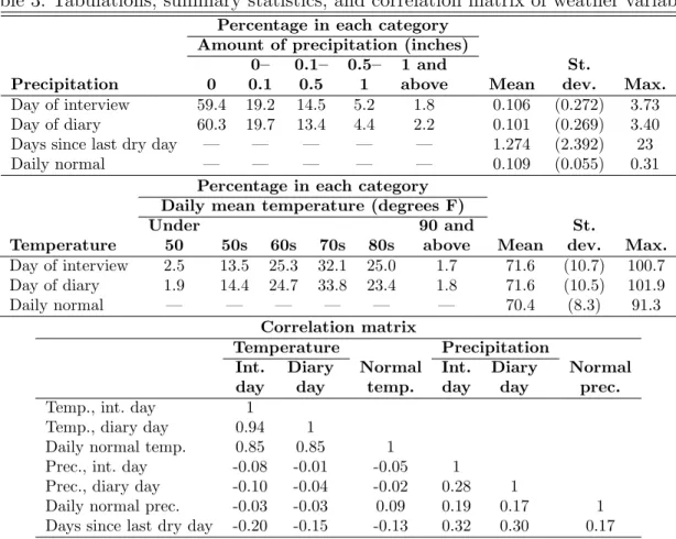
Data on the weather were added to the PATS data. The data on weather come from the Na-tional Climatic Data Center (NCDC) of the NaNa-tional Oceanic and Atmospheric Administration (NOAA).21 The daily summaries from over 8,000 weather stations located across the United States were used, corresponding to the data sets 3200 and 3210. The normal temperatures and precipi-tation levels come from the data set CLIM84, which is based on the weather from 1971 to 2000. Each respondent to the PATS was identified by his or her county of residence and matched to the average weather over all the weather stations in his or her county. Weather for the day of the interview and for the day of the diary (the day preceding the interview) was carefully identified. Because the PATS was conducted from May to August, snow is not significant to the study, so the elements used in this study are temperature and precipitation. Table 3 contains tabulations and summary statistics for the precipitation and temperature variables. For the purpose of the analysis, both rain and temperature were broken down in categorical variables, for which the breakdown is shown in Table 3. Days since last dry day counts the number of days from the day of the interview since it last rained, and is equal to zero if there is precipitation on the day of the interview. This
variable is meant to capture the effect of long rain spells, but its coefficient never comes out sta-tistically significant. While it is possible to look at the effect of both rain the day of the interview and the day of the diary (the day preceding the interview), the high day-to-day correlation for temperatures made it impossible to look at both the temperature of the interview day and of the diary day. Whenever temperature was used in regressions, I used temperature of the day of the interview when looking at satisfaction questions, and temperature of the day of the time-use diary (the day prior to the interview) when looking at feelings questions. The rationale was that for satisfaction questions, the previous day’s temperature should not matter, whereas when looking at feelings during specific episodes, it is the temperature at that time, and so on the diary day, that should matter. In any case, using either temperature does not change the results significantly, since the correlation between one day’s mean temperature and the previous day’s is 0.94, as can be seen in Table 3. In contrast, the same correlation for precipitation is 0.28.
4
Findings
4.1
Affect
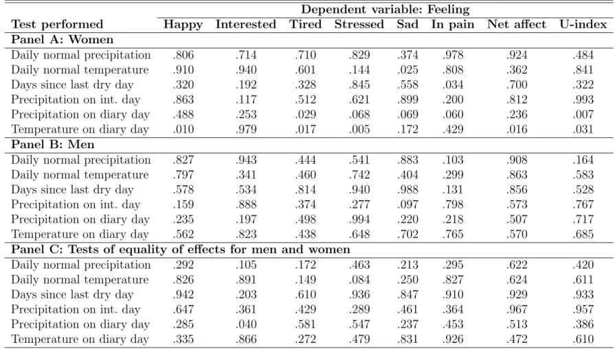
All the analyses were performed separately for men and women, and then jointly to test if the effects are indeed statistically different for men and women. Table 4 will only present test results for the significance of the weather variables, and the reader should refer to the online appendix for complete results for all regressions used in this paper as well as for coefficient estimates for the control variables. Looking at the effect of temperature, the omitted category is that of mean temperature in the 70s, which is what the average is.22That category was omitted to highlight the effect of extreme temperatures on feelings intensity.23 Examination of the analyses for women in Panel A reveals that temperature on diary day has a significant effect on the feelings happy, tired and stressed, as well as on the net affect and U-index. While not reported here,24 I found that low temperatures increase positive affect and decrease negative ones: low temperatures raise happiness and high ones lower it, and lower temperatures decrease tiredness, stress, and to a lesser extent sadness, and relatively high temperatures marginally increase the intensity of sadness. All this leads to a rise in net affect for very low temperatures and a decrease for very high temperatures.
22The same analysis was done using maximum temperature instead of mean temperature. The two are so highly
correlated however (correlation over 0.95) that the results are the same, just shifted up by 10 degrees, the average difference between mean and max temperatures.
23Note that the analyses were also done using a specification with normal weather and deviations from normal
weather, instead of levels of precipitation and temperature. The results did not change qualitatively, and are more easy to interpret in the format presented here.
These effects are also large: a day with temperature above 90 (relative to one in the 70s) has a bigger effect on the net affect than being divorced or widowed (relative to being married), and a day under 50 has an effect almost twice the size of that of being married (relative to being divorced),25 which is about half a standard deviation of the net affect. Since the Princeton Affect and Time Survey was conducted in summer months, this seems reasonable, and is also consistent with the evidence found by Rehdanz and Maddison (2005) and Keller et al. (2005).
When thinking about precipitation my prior is that precipitation on the day of the diary (that is, when the activity was taking place) is what would be important, not precipitation on the interview day. This is indeed true: whenever significant (for the feelings tired, stressed, sad and in pain and the U-index), it is rain on the diary day that matters. What is surprising is the direction of the effects: more rain seems to be linked with less tiredness, stress and sadness, though mostly for the higher levels of precipitation.26 Perhaps when asked about tiredness on rainy days, survey respondents attribute their tiredness to the rain and thus ‘factor out’ the rain in their answer.
The findings for men reported in Panel B are striking: none of the tests come out statistically significant at the usual levels of significance, except one that is marginally significant with a p-value of 0.097. Men do not appear to respond to weather shocks the same way women do. Panel C shows the tests of equality between men and women, where a low p-value means that equality is rejected. Looking at Panel C, most tests conclude that we cannot reject the hypothesis that men and women behave alike. This may be because men’s estimates are imprecise.
4.2
Satisfaction
The PATS data include four general satisfaction questions, relating to different spheres of life: life overall, life at home, health, and job satisfaction. Table 5 presents regression estimates for the effect of weather on life satisfaction for women. Column (1) of Table 5 is with month fixed effects while column (2) adds state fixed effects. My prior, and contrary to the feelings questions, is now that if rain has an effect on satisfaction levels, it would be the rain of the day of the interview, not of the diary day (the day before the interview, for which the time-use diary is collected). None of the rain dummies for the diary day are significant, but most of the ones for the interview day are, all reducing satisfaction level more or less monotonically (the omitted category is that of no rain at all). Further confirming my hypothesis, the F-statistics and their associated p-values presented at the bottom of the table show that taken together, the rain dummies for the interview day are significant but not the ones for the diary day.
25Argyle (1999) reported that “Marriage has often been found to be one the strongest correlates of happiness and
well-being.” (p. 359)
26The coefficients for precipitation more than 0 but less than 0.1 inch are of the expected sign, though not
Turning to temperature, I found that lower temperatures are associated with higher satisfaction (though the effects are not statistically significant) while higher temperatures negatively impact life satisfaction, both statistically and substantively: a temperature in the 80s (compared to the 70s) decreases life satisfaction by about 2 standard deviations, and in the 90s by 2 to 3 standard deviations, depending if the state fixed effects are included or not. Moreover, the decrease in satisfaction linked to temperature in the 90s is of a similar size as the decrease due to being single (relative to being married). Taken together, however, the temperature dummies are only marginally statistically significant in the specification without state fixed effects, and not at all for that including state fixed effects.
Daily normal mean temperature has a positive but small impact on life satisfaction. Daily normal precipitation significantly decreases life satisfaction, with an extra a standard deviation of normal rain reducing life satisfaction 5%-10% of a standard deviations. The biggest change in estimates between column (1) and column (2) (adding state fixed effects) is for the coefficient on normal precipitation. This is not so surprising since the normal reflects the time of year and the geographical location of the individual. Changes in normal precipitation within state are likely to be smaller.
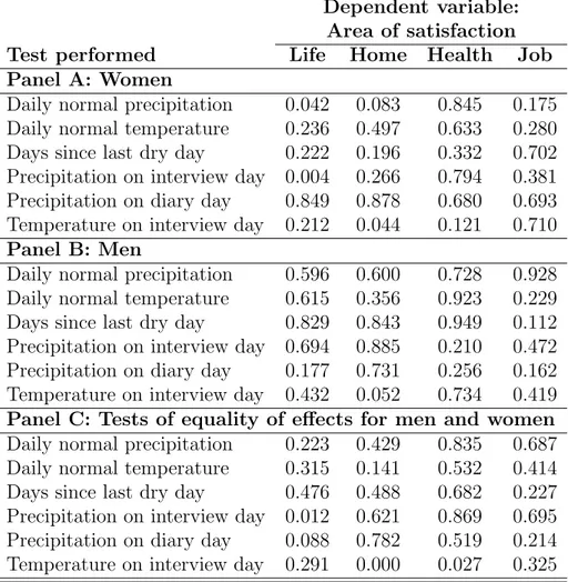
Table 6 is similar to Table 4 in showing test results for the joint significance of weather variables, but now for regressions (including month and state fixed effects) where areas of satisfaction are the dependent variables. Panel A reports the test results for women only, so the first column (Life) corresponds to the results from Table 5, column (2). Looking at the rest of Panel A, we can observe that only one other relation appears statistically significant (at a level of 5% or less): that of the effect of temperature on home satisfaction. We see in Panel B the results for men, and conclude once again that none of the variables have an impact on men’s satisfaction reports. The only group of variables that is jointly significant at a level under 10% is again the one for the temperature on the interview day.27 Panel C shows the results of tests of equality of effects between men and women: only for the effect of precipitation on interview day on life satisfaction and the effect of temperature on home satisfaction are the effects different.
In conclusion, weather the day of the interview seems to affect only women, with more rain and higher temperatures statistically and substantively decreasing life satisfaction, consistent with the affect results. Interestingly, the same patterns do not emerge when considering other aspects of satisfaction, which would support the hypothesis that women resort to their weather-influenced mood as “reasonable and parsimonious indicator” only for the most global of evaluations (life vs.
27For both men and women, the only temperature variable having a statistically significant impact is that for a
specific satisfaction). Men do not appear to let transient weather shocks influence their subjective satisfaction reports, which could be because of the weaker effect of weather on their mood that is found with the affect data. It could also be, as in Connolly (2008), that men respond more to the weather by modifying their activities, thus mitigating the effect on their subjective well-being.
5
Conclusion
In this paper, subjective well-being data from the Princeton Affect and Time Survey, the PATS, were supplemented by weather data to investigate the effect of precipitation and temperature, both transitory and average, on satisfaction levels and feelings intensities. Overall, women appear more responsive to environmental variables, showing lower life satisfaction on rainier days. Satisfaction in the specific areas of the PATS, home, health and job, is much less influenced by rain, consistent with the hypothesis that the more general the evaluation asked of the respondent, the more she will rely on current mood to construct her judgment. The effect of the daily normals has to be interpreted carefully however: whereas the rain and temperature on a given day can be considered exogenous and arguably have a causal effect, the normals are not, and are subject to selection bias if people move to certain areas because of the weather, a claim supported by Rappaport (2007). Temperatures have the greatest effect on the intensity of happiness, tiredness, and stress, and thus show up in the net affect and U-index results too. Low temperatures provide the biggest boost, which since the PATS was run in the summer months, from May to August, seems a reasonable finding. It would be interesting to compare this with results coming from data collected in the winter, to see if the effect is reversed, as suggested in Rehdanz and Maddison (2005) and Keller et al. (2005). There is some evidence that rain reduces tiredness and stress, which in turn reduces the U-index associated with heavy rain. The results for men are simply not robust enough for any clear conclusion to be drawn from this study on the responsiveness of men’s satisfaction levels and feelings to the weather, and suggest that they do not respond to weather shocks the same way women do.
If the past few years are any predictor of the direction future research in economics will take, then we can expect to see more studies incorporating subjective well-being data in their analysis. Knowing how such data are sensitive to elements like the temperature and amount of rain is important if researchers want to tease out the effect of transitory shocks to the weather, to focus on other variables and circumstances of interest. This paper provides evidence that current conditions will matter more to women than to men, and that simply controlling for month and state will not be sufficient to control for fluctuations around normal conditions and day-to-day variations. If a researcher’s data come from a year-round, country-wide survey, it could be reasonable to think
that weather shocks are essentially random and would not bring significant bias one or way the other. But if SWB data are collected over a short period of time and in a specific location, one needs to be careful about interpretation of regression estimates, especially when making gender comparisons, since one conclusion we can draw from this study is that women’s SWB is generally more affected by weather than men’s. One way to deal with this situation would be to include weather data in the analysis, which is reasonable especially if the survey is covering only a few days and/or locales. If weather shocks affect mood which affects life satisfaction, the problem may be seen as one of too much noise (weather shocks) for the amount of signal (‘real’ satisfaction). One way to reduce the noise would be to use priming about the weather in the questionnaire, that is inducing survey respondents not to rely on the meteorological condition as a “parsimonious indicator” of satisfaction, as Schwarz and Clore (1983) have shown. In surveys where adding a question comes with a premium, this may unfortunately not be possible, and the econometrician will have to be careful about interpretation. One question left unanswered by this study and for which the PATS could help, with its information on well-being and time use combined, is that of the transmission channel of the weather effects. Does the weather directly influence SWB, or is it mostly that weather affects activities, which then affect mood and SWB in general? Answering this question may also help shed light on the gender differences in responses to weather documented in this paper.
References
Argyle, Michael (1999), “Causes and Correlates of Happiness,” in Well-Being: The Foun-dations of Hedonic Psychology, Daniel Kahneman, Ed Diener and Norbert Schwarz, eds., Russell Sage Foundation, New York, NY, 353–373.
Argyle, Michael (2001), The Psychology of Happiness, 2nd edition, Routledge, Taylor & Francis Inc., New York, NY, 276 pages.
Argyle, Michael and Maryanne Martin (1991), “The Psychological Causes of Happi-ness,” in Subjective Well-Being. An Interdisciplinary Perspective, Fritz Strack, Michael Argyle and Norbert Schwarz, eds., Pergamon Press, Oxford, England, 77–100.
Barrington-Leigh, Christopher (2008), “Weather as a transient influence on survey-reported satisfaction with life,” Draft research paper, University of British Columbia, August 2008.
Bok, Derek (2010), The Politics of Happiness: What Government Can Learn from the New Research on Well-Being, Princeton University Press, Princeton, NJ, 272 pages.
Connolly, Marie (2008), “Here Comes the Rain Again: Weather and the Intertemporal Substitution of Leisure,” Journal of Labor Economics 26 (1): 73–100.
Cunningham, Michael R. (1979), “Weather, Mood, and Helping Behavior: Quasi Ex-periments with the Sunshine Samaritan,” Journal of Personality and Social Psychology 37 (11): 1974–1956.
Denissen, Jaap J. A., Ligaya Butalid, Lars Penke and Marcel A.G. van Aken (2008), “The Effects of Weather on Daily Mood: A Multilevel Approach,” Emotion 8 (5): 662–667. Diener, E., R. Lucas, U. Schimmack and J.F. Helliwell (2009), Well-Being for Public Policy, Oxford University Press, New York, NY.
Dowling, Michael and Brian M. Lucey (2005), “Weather, Biorhythms, Beliefs and Stock Returns—Some Preliminary Irish Evidence,” International Review of Financial Analysis 14 (3): 337–355.
Frey, Bruno S. and Alois Stutzer (2002), “What Can Economists Learn from Happi-ness Research?” Journal of Economic Literature 40 (2): 402–435.
Goetzmann, William N. and Ning Zhu (2003), “Rain or Shine: Where Is the Weather Effect?” Working Paper No. 9,465, National Bureau of Economic Research, Cambridge, MA. Helliwell, John F. and Christopher P. Barrington-Leigh (2010), “Measuring and Un-derstanding Subjective Well-Being,” Working Paper No. 15,887, National Bureau of Economic Research, Cambridge, MA.
Hirshleifer, David and Tyler Shumway (2003), “Good Day Sunshine: Stock Returns and the Weather,” The Journal of Finance 58 (3): 1009–1032.
Kahneman, Daniel, Ed Diener and Norbert Schwarz, eds. (1999), Well-Being: The Foundations of Hedonic Psychology, The Russell Sage Foundation, New York, NY, 593 pages. Kahneman, Daniel and Alan B. Krueger (2006), “Developments in the Measurement of Subjective Well-Being,” Journal of Economic Perspectives 20 (1): 3–24.
Kahneman, Daniel, Alan B. Krueger, David A. Schkade, Norbert Schwarz and Arthur A. Stone (2004), “A Survey Method for Characterizing Daily Life Experience: The Day Reconstruction Method,” Science 26 (3 December 2004): 1776–1780.
Keller, Matthew C., Barbara L. Fredrickson, Oscar Ybarra, St´ephane Cˆot´e, Kareem Johnson, Joe Mikels, Anne Conway and Tor Wager (2005), “A Warm Heart and a Clear Head. The Contingent Effects of Weather on Mood and Cognition,” Psychological Science 16 (9): 724–731.
Krueger, Alan B., ed. (2009), Measuring the Subjective Well-Being of Nations. Na-tional Accounts of Time Use and Well-Being, NaNa-tional Bureau of Economic Research Conference Report, The University of Chicago Press, Chicago, IL, 262 pages.
Krueger, Alan B., Daniel Kahneman, David Schkade, Norbert Schwarz and Arthur A. Stone (2009), “National Time Accounting: The Currency of Life,” in Measuring the Subjec-tive Well-Being of Nations. National Accounts of Time Use and Well-Being, Alan B. Krueger ed., National Bureau of Economic Research Conference Report, The University of Chicago Press, Chicago, IL, 9–86.
OECD (2011), Compendium of OECD Better Life Indicators, OECD Better Life Ini-tiative, available online at http://www.oecd.org/dataoecd/4/31/47917288.pdf (accessed May 26, 2011).
Oren, D. A. and N. E. Rosenthal (1992), “Seasonal Affective Disorder,” in Handbook of Affective Disorders, 2nd edition, E. S. Paykel, ed., Guilford, New York, NY, 551–568. Rappaport, Jordan (2007), “Moving to Nice Weather,” Regional Science and Urban Economics 37 (2007): 377–398.
Rehdanz, Katrin and David Maddison (2005), “Climate and Happiness,” Ecological Economics 52 (2005): 111–125.
Rind, Bruce (1996), “Effects of Beliefs About Weather Conditions on Tipping,” Jour-nal of Applied Social Psychology 26 (2): 137–147.
Rind, Bruce and David Strohmetz (2001), “Effect of Beliefs About Future Weather Conditions on Restaurant Tipping,” Journal of Applied Social Psychology 31 (10): 2160–2164. Saunders, Edward M. Jr. (1993), “Stock Prices and Wall Street Weather,” American Economic Review 83 (5): 1337–1345.
Schkade, David A. and Daniel Kahneman (1998), “Does living in California make peo-ple happy? A focusing illusion in judgments of life satisfaction,” Psychological Science 9 (5): 340–346.
Schwarz, Norbert and G.L. Clore (1983), “Mood, Misattribution, and Judgments of Well-being: Informative and Directive Functions of Affective States,” Journal of Personality and Social Psychology 45 (3): 513–523.
Schwarz, Norbert and Fritz Strack (1991), “Evaluating one’s life: a judgment model of subjective well-being,” in Subjective Well-Being. An Interdisciplinary Perspective, Strack, Fritz, Michael Argyle and Norbert Schwarz, eds., Pergamon Press, Oxford, England: 27–47. Simonsohn, Uri (2007), “Clouds Make Nerds Look Good: Field Evidence of The
Im-pact of Incidental Factors on Decision Making,” Journal of Behavioral Decision Making 20 (2): 143–152.
Smith, Tom W. (1979), “Happiness: Time Trends, Seasonal Variations, Intersurvey Differences, and Other Mysteries,” Social Psychology Quarterly 42 (1): 18–30.
Stiglitz, Joseph E., Amartya Sen and Jean-Paul Fitoussi (2009), Report by the Com-mission on the Measurement of Economic Performance and Social Progress, available online at www.stiglitz-sen-fitoussi.fr.
Strack, Fritz, Michael Argyle and Norbert Schwarz, eds. (1991), Subjective Well-Being. An Interdisciplinary Perspective, Pergamon Press, Oxford, England, 291 pages.
Table 1: Tabulations and summary statistics of feelings variables
Panel A: Women Percentage in each category Feeling intensity
Feeling or variable 0 1 2 3 4 5 6 Mean St. dev N
Happy 6.0 3.1 6.5 14.8 17.6 23.5 28.5 4.19 (1.73) 7,024 Interested 8.3 4.1 8.1 14.2 16.8 19.0 29.5 4.02 (1.88) 7,025 Tired 25.0 7.6 11.1 14.5 14.7 14.2 13.0 2.81 (2.12) 7,039 Stressed 48.7 11.2 11.6 9.1 7.1 6.1 6.2 1.58 (1.95) 7,038 Sad 76.8 7.1 4.8 3.9 2.6 1.9 2.9 0.66 (1.46) 7,037 In pain 73.2 5.1 4.4 4.7 4.3 4.2 4.1 0.91 (1.74) 7,038 Net affect — — — — — — — 3.14 (2.47) 7,012 U-index — — — — — — — 0.20 (0.40) 7,012
Panel B: Men Percentage in each category Feeling intensity
Feeling or variable 0 1 2 3 4 5 6 Mean St. dev N
Happy 4.9 2.4 7.5 19.5 20.5 22.6 22.6 4.06 (1.62) 4,316 Interested 5.9 3.9 8.3 16.1 19.2 22.3 24.4 4.03 (1.73) 4,319 Tired 26.2 10.2 14.1 15.7 14.4 11.6 7.8 2.48 (1.99) 4,322 Stressed 47.4 14.0 13.8 9.6 6.2 4.7 4.4 1.45 (1.79) 4,319 Sad 73.4 10.1 6.4 4.1 2.6 1.7 1.7 0.64 (1.33) 4,324 In pain 71.3 6.8 6.3 5.3 4.6 2.5 3.2 0.85 (1.61) 4,321 Net affect — — — — — — — 3.08 (2.24) 4,307 U-index — — — — — — — 0.18 (0.38) 4,307
Note: Weighted by sample weights. Feeling intensity questions are rated on a scale of 0 to 6, with 0 representing a low intensity, and 6 a high intensity. Net affect is the intensity of happiness minus the average of stressed, sad, and pain. The U-index is 1 if stressed, sad, or pain is greater than happy and 0 otherwise.
Table 2: Tabulations and summary statistics of satisfaction variables
Panel A: Women Percentage in each category
Area of Not at all Not Very St.
satisfaction satisfied satisfied Satisfied satisfied Mean dev. N
Life 1.68 9.51 43.58 45.24 3.32 (0.71) 2,347
Home 1.28 7.91 43.47 47.34 3.37 (0.68) 2,349
Health 4.82 18.62 46.91 29.64 3.01 (0.82) 2,345
Job 2.35 13.13 53.07 31.45 3.14 (0.72) 1,062
Panel B: Men Percentage in each category
Area of Not at all Not Very St.
satisfaction satisfied satisfied Satisfied satisfied Mean dev. N
Life 1.39 9.25 46.73 42.64 3.31 (0.69) 1,444
Home 1.18 5.81 42.21 50.80 3.43 (0.66) 1,445
Health 2.92 16.48 51.76 28.84 3.07 (0.75) 1,449
Job 2.46 14.00 51.82 31.71 3.13 (0.73) 879
Note: Weighted by sample weights. Satisfaction questions are rated on a scale of 1 to 4, with 1 meaning “Not at all satisfied,” and 4 meaning “Very satisfied.”
Table 3: Tabulations, summary statistics, and correlation matrix of weather variables
Percentage in each category Amount of precipitation (inches)
0– 0.1– 0.5– 1 and St.
Precipitation 0 0.1 0.5 1 above Mean dev. Max.
Day of interview 59.4 19.2 14.5 5.2 1.8 0.106 (0.272) 3.73 Day of diary 60.3 19.7 13.4 4.4 2.2 0.101 (0.269) 3.40 Days since last dry day — — — — — 1.274 (2.392) 23
Daily normal — — — — — 0.109 (0.055) 0.31
Percentage in each category Daily mean temperature (degrees F)
Under 90 and St.
Temperature 50 50s 60s 70s 80s above Mean dev. Max. Day of interview 2.5 13.5 25.3 32.1 25.0 1.7 71.6 (10.7) 100.7 Day of diary 1.9 14.4 24.7 33.8 23.4 1.8 71.6 (10.5) 101.9
Daily normal — — — — — — 70.4 (8.3) 91.3
Correlation matrix
Temperature Precipitation
Int. Diary Normal Int. Diary Normal
day day temp. day day prec.
Temp., int. day 1
Temp., diary day 0.94 1
Daily normal temp. 0.85 0.85 1
Prec., int. day -0.08 -0.01 -0.05 1
Prec., diary day -0.10 -0.04 -0.02 0.28 1
Daily normal prec. -0.03 -0.03 0.09 0.19 0.17 1 Days since last dry day -0.20 -0.15 -0.13 0.32 0.30 0.17
Note: Weighted by sample weights. Precipitation is measured in inches. Days since last dry day counts the number of days since it last rained, and is equal to zero if the interview day is rainy. Temperature is mean daily
temperature (the average of the minimum and the maximum temperatures for the day), in degrees Fahrenheit. Normals are daily normals (see Data section for details).
Table 4: Test results of significance of weather variables in feelings regressions Dependent variable: Feeling
Test performed Happy Interested Tired Stressed Sad In pain Net affect U-index
Panel A: Women
Daily normal precipitation .806 .714 .710 .829 .374 .978 .924 .484
Daily normal temperature .910 .940 .601 .144 .025 .808 .362 .841
Days since last dry day .320 .192 .328 .845 .558 .034 .700 .322
Precipitation on int. day .863 .117 .512 .621 .899 .200 .812 .993
Precipitation on diary day .488 .253 .029 .068 .069 .060 .236 .007
Temperature on diary day .010 .979 .017 .005 .172 .429 .016 .031
Panel B: Men
Daily normal precipitation .827 .943 .444 .541 .883 .103 .908 .164
Daily normal temperature .797 .341 .460 .742 .404 .299 .863 .583
Days since last dry day .578 .534 .814 .940 .988 .131 .856 .528
Precipitation on int. day .159 .888 .374 .277 .097 .798 .573 .767
Precipitation on diary day .235 .197 .498 .994 .220 .218 .507 .717
Temperature on diary day .562 .823 .438 .648 .702 .765 .570 .685
Panel C: Tests of equality of effects for men and women
Daily normal precipitation .292 .105 .172 .463 .213 .295 .622 .420
Daily normal temperature .826 .891 .149 .084 .250 .827 .624 .611
Days since last dry day .942 .203 .610 .936 .847 .910 .929 .933
Precipitation on int. day .647 .361 .429 .289 .461 .364 .967 .957
Precipitation on diary day .285 .040 .581 .547 .237 .453 .513 .386
Temperature on diary day .335 .866 .272 .479 .831 .926 .472 .610
Note: All values listed are p-values (Prob. > F) of the corresponding F-test of the (joint) significance of the variables listed. Each regression also includes controls for education, age and age squared, marital status, race, and hispanic ethnicity, with fixed effects for day of week, activity, month and state. Weighted by sample weights. The standard errors are clustered at the individual level.
Table 5: Regression results, effect of weather on life satisfaction, women
Dependent variable: Life satisfaction
Independent variable (1) (2)
Daily normal prec. -0.827** -1.462**
(0.340) (0.698)
Precipitation on interview day
0 < prec. < 0.1 -0.106** -0.094* (0.050) (0.050) 0.1 6 prec. < 0.5 -0.110* -0.100 (0.061) (0.061) 0.5 6 prec. < 1 -0.170** -0.162* (0.084) (0.090) 1 6 prec. -0.332** -0.319** (0.135) (0.149)
Precipitation on diary day (day before interview)
0 < prec. < 0.1 0.011 -0.028 (0.048) (0.049) 0.1 6 prec. < 0.5 -0.016 -0.043 (0.055) (0.050) 0.5 6 prec. < 1 -0.002 -0.033 (0.086) (0.091) 1 6 prec. 0.067 0.029 (0.130) (0.130)
Days since last dry day 0.009 0.012
(0.009) (0.009)
Daily normal temp. 0.012** 0.010
(0.005) (0.009)
Temperature on interview day
Under 50 0.171 0.201 (0.156) (0.162) 50s 0.032 0.021 (0.078) (0.076) 60s -0.025 -0.031 (0.053) (0.050) 80s -0.169*** -0.158** (0.061) (0.065) 90 and above -0.234*** -0.155 (0.080) (0.107) Constant 3.435*** 3.668*** (0.396) (0.642) R-squared 0.104 0.132
Month fixed effects x x
State fixed effects x
F-test prec. int. day 5.826 4.392
Prob. > F prec. int. day 0.001 0.004
F-test prec. diary day 0.116 0.341
Prob. > F prec. diary day 0.976 0.849
F-test temp. int. day 1.985 1.486
Prob. > F temp. int. day 0.098 0.212
Note: Clustered standard errors in parentheses (at state level). * significant at 10%; ** significant at 5%, *** significant at 1%. Precipitation is measured in inches, mean temperature in degrees Fahrenheit. Omitted categories are no rain and mean temperature in the 70s. The regressions also include controls for education, age and age squared, marital status, race, and hispanic ethnicity. The F-tests are of the joint significance of the precipitation and temperature dummies. Weighted by sample weights. N = 2,062
Table 6: Test results of significance of weather variables in satisfaction regressions Dependent variable:
Area of satisfaction
Test performed Life Home Health Job
Panel A: Women
Daily normal precipitation 0.042 0.083 0.845 0.175
Daily normal temperature 0.236 0.497 0.633 0.280
Days since last dry day 0.222 0.196 0.332 0.702
Precipitation on interview day 0.004 0.266 0.794 0.381
Precipitation on diary day 0.849 0.878 0.680 0.693
Temperature on interview day 0.212 0.044 0.121 0.710
Panel B: Men
Daily normal precipitation 0.596 0.600 0.728 0.928
Daily normal temperature 0.615 0.356 0.923 0.229
Days since last dry day 0.829 0.843 0.949 0.112
Precipitation on interview day 0.694 0.885 0.210 0.472
Precipitation on diary day 0.177 0.731 0.256 0.162
Temperature on interview day 0.432 0.052 0.734 0.419
Panel C: Tests of equality of effects for men and women
Daily normal precipitation 0.223 0.429 0.835 0.687
Daily normal temperature 0.315 0.141 0.532 0.414
Days since last dry day 0.476 0.488 0.682 0.227
Precipitation on interview day 0.012 0.621 0.869 0.695
Precipitation on diary day 0.088 0.782 0.519 0.214
Temperature on interview day 0.291 0.000 0.027 0.325
Note: All values listed are p-values (Prob. > F) of the corresponding F-test of the (joint) significance of the variables listed. Each regression also includes controls for education, age and age squared, marital status, race, and hispanic ethnicity, with fixed effects for month and state. Weighted by sample weights. The standard errors are clustered at the state level.