Distribution and variability study of the femur cortical thickness from computer tomography

is an open access repository that collects the work of Arts et Métiers Institute of

Technology researchers and makes it freely available over the web where possible.

This is an author-deposited version published in: https://sam.ensam.eu

Handle ID: .http://hdl.handle.net/10985/20222

To cite this version :

Antoine SERRURIER, Erwan JOLIVET, Sergio QUIJANO, Patricia THOREUX, Wafa SKALLI Distribution and variability study of the femur cortical thickness from computer tomography -Computer Methods in Biomechanics and Biomedical Engineering - Vol. 17, n°7, p.768-786 - 2012

Any correspondence concerning this service should be sent to the repository Administrator : archiveouverte@ensam.eu

Distribution and variability study of the femur cortical thickness from computer tomography

Arts et Me´tiers ParisTech, Laboratoire de Biome´canique, 151 bd de l’Hoˆpital, 75013 Paris, France (Received 30 June 2011; final version received 23 July 2012)

In the context of patient-specific 3D bone reconstruction, enhancing the surface with cortical thickness (COT) opens a large field of applications for research and medicine. This functionality calls for database analysis for better knowledge of COT. Our study provides a new approach to reconstruct 3D internal and external cortical surfaces from computer tomography (CT) scans and analyses COT distribution and variability on a set of asymptomatic femurs. The reconstruction method relies on a short (,5 min) initialisation phase based on 3D reconstruction from biplanar CT-based virtual X-rays and an automatic optimisation phase based on intensity-based cortical structure detection in the CT volume, the COT being the distance between internal and external cortical surfaces. Surfaces and COT show root mean square reconstruction errors below 1 and 1.3 mm. Descriptions of the COT distributions by anatomical regions are provided and principal component analysis has been applied. The first mode, 16 – 50% of the variance, corresponds to the variation of the mean COT around its averaged shape; the second mode, 9 – 28%, corresponds to a fine variation of its shape. A femur COT model can, therefore, be described as the averaged COT distribution in which the first parameter adjusts its mean value and a second parameter adjusts its shape.

Keywords: bone cortical thickness; human femur; 3D reconstruction; biomedical imaging; CT; bone modelling

1. Introduction

In the last decades, the progress on medical images coupled with innovative engineering techniques allowed the developments of patient-specific three-dimensional (3D) skeleton reconstruction used in clinical routine. In particular, 3D bone reconstructions from biplanar radio-graphs showed an increasing interest both for research and medical purposes (Laporte et al.2003; Humbert et al.2009; Zheng et al.2009; Jolivet et al.2010; Chaibi et al.2011). The various personalised 3D reconstructions presented in the literature remain, however, limited to surface reconstructions of the bone without modelling of the volume itself. In particular, no further information is provided on the cortical structure of the bone, although the radiographs depend largely on the quantity of cortical bone crossed by the X-rays. For the case of the femur, this lack of cortical bone reconstruction might be ascribed to the lack of knowledge on the cortical thickness (COT) distribution and variability across the population. However, the knowledge of the COT distribution and its personalised reconstruction for patients appear of great importance for research and medical purpose. Indeed, the cortical bone constitutes a solid cast around the bone and counts for a major structure in the strength of the bone. Medical and research applications dealing with mechanical modelling of the bone may benefit a precise COT map in addition to the patient-specific 3D geometry. We shall cite in that domain risk fracture prediction for asymptomatic subjects or

osteoporotic patients which constitutes nowadays a major medical and economic challenge. Similarly, the design of hip prosthesis depends largely on the COT of the proximal femur and may also benefit of precise COT maps for the patients. On another note, our recent research led us to compute virtual X-rays of the femur in the process of automation of the 3D surface reconstruction from biplanar X-rays (Serrurier et al. 2012). These virtual X-rays are obtained by simulating the X-ray propagation through the 3D reconstruction of the femur, in which the attenuation of the ray depends on the bone structure. We have shown that a bone divided into two structures, one cortical and one spongy, lead to satisfactory results. Such process and the previous applications call for a better knowledge of the COT distribution of the femur.

Although a large part of the research on the internal femur structure has been focused on the bone mineral density, various studies have considered the cortical bone structure. Various approaches have been considered depending on the purpose of the research, e.g. for osteoporosis (Barnett and Nordin 1960; Virtama and Telkka1962; Treece et al.2010; Poole et al.2011), fracture risk estimation and relation with age (Smith et al. 1982; Noble et al.1995; Ho¨gler et al.2003; Mayhew et al.2005; Bousson et al. 2006), surgery planning and prosthesis design or insertion (Robertson et al.1987; Noble et al.1988; Sugano et al.1998; Stephenson and Seedhom1999; Adam et al.2002; Seebeck et al.2004), bone regeneration (Bra˚ten

q_{2012 Taylor & Francis}

*Corresponding author. Email:antoine.serrurier@ensam.eu

et al. 1992), death age estimation (Chan et al. 2007) or palaeontology (Croker et al.2009). Many of these studies consider the COT of the femur on limited locations of the bone. Most of them focus on the diaphysis, whose COT is accurately measurable on perpendicular sections (e.g. Laine et al.1997; Stephenson and Seedhom1999; Croker et al.2009), as emphasised by the definition of a COT score by Barnett and Nordin (1960). A more limited number of studies focus on the proximal femur (e.g. Noble et al.1988; Adam et al.2002) and more precisely on the neck, in the context of fracture risk. To our knowledge, the most complete studies are those of Treece et al. (2010) and Poole et al. (2011) on the proximal femur. Treece et al. (2010) propose a method to obtain the COT distribution of the proximal femur from computer tomography (CT) scans with a sub-millimetre precision for thin thicknesses. They provide in their article a few sample of 3D surfaces of the proximal femur augmented with COT distribution, whereas Poole et al. (2011) rely on this method to monitor the regeneration of cortical bone in vivo.

However, as far as we know, no description of the COT distribution on the full femur has been provided in the literature and no variability study of this distribution has been carried out. This may be ascribed by the difficulty to gather complete sets of image data for several subjects and to the processing complexity to extract the information. Our objective in this study consists thus in filling this gap by describing the COT map of the femur and study its variability for asymptomatic subjects.

Types of recorded data are a key factor for accurate description of the COT of the femur. X-rays were largely used in the past to assess the cortical bone geometry of the femur diaphysis (e.g. Barnett and Nordin1960; Noble et al.

1995) but remain, however, inappropriate for the proximal and distal regions. The more recent development of CT scanning led researchers to compare the accuracy of COT estimation from radiography and CT scanning (e.g. Smith et al.1982) or even from MRI (Preidler et al.1997). Based on X-ray propagation, computer tomography provides axial scans of the body, allowing 3D recordings of the femur with high resolution. This technique, particularly adapted for the discrimination of cortical structures, has been largely adopted in the recent years for the study of the cortical bone (e.g. Robertson et al.1987; Laine et al.1997; Kang et al.2003; Treece et al.2010; Poole et al.2011). Although some limitations were emphasised in the past (see e.g. Hangartner and Gilsanz 1996; Prevrhal et al.

1999), we chose to rely on CT scans of the femur for this study, which appears to be the appropriate technique to assess COT according to the literature.

Considering the large amount of work to extract manually, the boundaries of the internal and external cortical structures from CT scans, automatic or semi-automatic methods must be considered. Kang et al. (2003) propose a reconstruction method based on traditional

segmentation techniques. Although not applied to the full femur, they appear to provide interesting results with a limited interaction of the operator. More recently, Treece et al. (2010) have provided another method based on intensity profile interpretation to extract the internal cortical surface once the external cortical surface is already segmented by semi-automatic techniques. In this study, we aimed to provide an alternative method to extract both internal and external cortical surfaces from the CT scans, by taking full advantage of the recent developments on 3D surface reconstruction from biplanar X-rays (Chaibi et al.

2011). This method intends to be a robust alternative to image segmentation techniques and fully automatic for both surfaces after a very limited manual initialisation by the operator. This method is presented in Section 2 of the paper. It will be applied to several sets of CT scans of the femur for several subjects and a description of the COT distribution is provided in Section 3. The variability across the database will be investigated by means of principal component analysis (PCA) and the results are presented in the same section.

2. Materials and methods 2.1 Subjects and data

Axial CT slices were collected at the Cochin hospital (Paris, France) from 15 cadavers between May 2007 and October 2009. The population consisted of 13 males and 2 females, with a mean age of 74.5 years, spanning from 56 to 88. The subjects were placed in a supine position, the arms along the body sides. Image sets of subjects having at least one side without hip and knee prosthesis were kept for the study. Fifteen left and 14 right femurs without visible osseous abnormalities on the images were finally selected for the study.

The axial CT slices of 0.75 mm thick were recorded from the feet to the head with an inter-slice distance of 0.5 mm. Images of size 512 £ 512 with pixel resolutions of 0.97 £ 0.97 mm2were available for the study. The sets of the images were restricted for the study: for each subject, images spanning only from below the knees until those above the hip were manually selected among the full body sets. A qualitative check of the selected images was finally carried out to ensure that the desired anatomy structures were selected, the images were correctly sorted and the general quality was satisfactory. Note that one femur was additionally discarded from the study because of a femoral neck almost invisible on the images.

In order to ensure an easier manipulation of the images along the study, the sets of images, encompassing the whole body from the knee to the pelvis, were manually cropped with the help of the software Amiraq. From each set of images, a restriction of the voxel volume around the desired femur was carried out, preserving the same image

resolution. Twenty-eight sets of images for the 28 femurs of the study were created this way.

2.2 3D reconstruction

The purpose consisted in building a database of 28 pairs of femur surfaces, the internal and the external cortical surfaces for each femur. Methods based on manual or semi-manual segmentation on each images have shown efficiency, but require high amount of manual work not adapted for database building. On the other side, recent works (Chaibi et al. 2011) have been focused on the 3D reconstruction from biplanar radiographs: the results have shown that 3D external cortical surface of the femur can be reconstructed with a root mean square (RMS) error of 1.2 mm within about 5 min. We propose in this section an original method to reconstruct the 3D internal and external cortical surface of the femur from CT scans based on these results: a first mesh of the external cortical surface is estimated from CT-based virtual biplanar radiographs by means of the reconstruction method proposed by Chaibi et al. (2011) and this mesh is adjusted on the CT scans by means of an automatic method, at the same time as the internal cortical surface is computed.

To serve as a reference and to evaluate the accuracy of this method, the internal and the external cortical surfaces of 10 femurs from our database have moreover been manually segmented on the CT scans by means of the software Amiraq

.

For the whole study, the origin of the reference coordinate system for each femur is provided by the CT scanner and extracted through the DICOM fields of the images and the axes provided by the orientations of the scans.

2.2.1 Initial estimation of the external femur surface Two calibrated biplanar digitally reconstructed radio-graphs (de Bruin et al. 2008) have been computed by

simulating the X-ray propagation through the CT sets, so as to simulate X-rays for biplanar face and lateral radiographs of the femur, as necessary inputs for the reconstruction method proposed by Chaibi et al. (2011). The 3D reconstructions of the external surface of the femur were carried out from the biplanar images according to this Chaibi and colleagues method. This initial solution is already quite accurate as the reported RMS reconstruc-tion error is 1.2 mm (Chaibi2010). The external cortical surface is represented as a closed triangular mesh (VRML format) made of 2372 vertices and 4740 triangles. The 3D surface model is already divided into regions such as the head, the neck, the diaphysis, the greater and lesser trochanters and the distal region. This initial reconstruc-tion, taking about 5 min by femur, is the only manual work requested from the operator.

2.2.2 Adjustment on the CT scans

The next step consisted in improving the accuracy of the reconstruction and estimating the internal cortical surface using the whole CT information. This process was carried out in an automatic way.

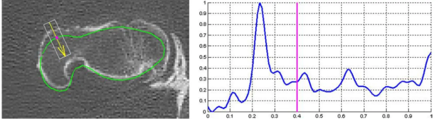
The process relies on the calculation of intensity functions. For a vertex of the reconstructed surface mesh, an intensity function is defined along the normal vector of the vertex as the averaged grey levels of the CT voxels embedded in a neighbourhood. The sets of images are considered only in 3D (bloc of voxels) and the intensity functions are computed in 3D but the process is illustrated in 2D inFigure 1for simplicity reasons.

By construction, as visible in Figure 1, an initial horizontal position of the external cortical surface is known for each intensity function, corresponding to the position of vertex from which is calculated the intensity function. In addition, an initial value of COT, obtained from a previous version of this study, is attributed to each

Figure 1. Left: CT scan superimposed with the contour obtained by the intersection of the initial 3D mesh with the image plane (green line), projections on the image plane of a vertex of this mesh (magenta point) and of a normal vector of this mesh along which is calculated an intensity function (yellow) and the rectangular neighbourhood within which is calculated the intensity function (white rectangle). Right: Vertically and horizontally normalised intensity function computed along the normal vector plotted on the left and within the rectangle. The vertical line on the intensity function marks the horizontal position of the initial external cortical vertex along the function.

vertex, providing also by consequence an initial position of the internal cortical surface on the intensity function. The objective of the following algorithm is to correct automatically their positions on the intensity function.

The algorithm consists in a recursive process in which the internal and/or external cortical positions correspond-ing to vertices for which a reliable solution could be found on the intensity functions have been kept, whereas the missing positions for the other vertices are interpolated. This is achieved by computing the positions of the 3D points corresponding to the retained intensity profile internal and external cortical positions, constituting the new target for the internal and external cortical surfaces. The initial meshes are then deformed towards this target by means of the kriging technique (Trochu1993), and the new intensity profiles are calculated for each vertex of the new meshes. This process allows a smooth convergence by discarding at each step the contribution of the vertices for which it is not possible to retrieve reliable internal and external cortical positions. The automatic detections of the internal and external cortical positions on the intensity profiles have been partially inspired by techniques used by Pan and Tompkins (1985) and Fokapu and Girard (1993) for electrocardiography signals processing. In short, their technique consists in detecting the extreme values on a signal obtained by adding the normalised first and second derivatives of the intensity profile, signal referred to as sum of the intensity derivativesin the following.

The recursive process contains five steps. Separate processing for the diaphysis vertices on one side and proximal and distal vertices on the other sides are performed. This has been motivated by the bigger COT of the diaphysis in comparison to the rest of the femur, ensuring a good visibility of this structure on the intensity profiles and consequently reliable detections obtained by simple threshold techniques. The five steps in between which are performed the deformation of the initial mesh towards the target, as mentioned above are the following: (1) the external cortical positions are adjusted by threshold detection of the rising edges of the intensity profile for a gross initial correction of the initial mesh; (2) the internal and external cortical positions for the proximal and distal vertices are adjusted by detecting the maximum and minimum values of the sum of the intensity derivatives; (3) the internal and external cortical positions for the proximal and distal vertices are centred around the maximum of the integral of the intensity function computed on a bandwidth corresponding to the COT value at this step; the positions for the diaphysis vertices are adjusted by threshold detection of the rising and falling edges of the intensity profile; (4) the internal and external cortical positions for all the vertices are adjusted by detecting the maximums of the second derivate of the intensity function and (5) the internal cortical position of the diaphysis vertices is adjusted on the falling edge of the intensity function. At

each step of the algorithm, more precise intensity functions are computed on a smaller length and with a smaller CT neighbourhood, so that to refine the process and to converge towards the solution.

The 3D reconstruction method proposed here was applied to the 28 sets of CT images of our database. Four cases presented segmentation errors, one in the greater trochanter region and three in the distal region, were discarded for the rest of the study. At the end of the process, we dispose of two meshes for each of the 24 femurs of the database: the internal and external surfaces of the cortical structure. An example of final result is given inFigure 2. Deriving from the femur mesh provided by Chaibi et al. (2011), these meshes have moreover a similar topology with the same number of vertices, and triangles are already divided into anatomic regions.

2.2.3 Evaluation

The accuracy of the reconstruction method was evaluated by the calculation of the point-to-surface distances between 10 sets of internal and external cortical structures and their reference meshes obtained by manual segmenta-tion. The mean, maximum and 2RMS distances, being calculated as twice the RMS distances and corresponding to 95% confidence intervals for normal distributions, were computed. In addition, the relative errors of the volume of the internal and external cortical meshes in relation to their reference meshes were computed. The volume of the cortical bone, computed as the difference between the volume of the external and internal cortical meshes, was assessed in the same way. The mean and maximum relative volume errors computed on the 10 femurs are provided.

2.3 Cortical thickness

To go further into bone thickness modelling, the COTs were computed, their distribution was characterised and the variability was studied by means of PCA.

2.3.1 Calculation

The COT was characterised in our study for six regions: the diaphysis, the neck, the head, the distal region, the greater trochanter and the lesser trochanter, as visible in

Figure 3.

For each femur, the COTs were computed as the distance between the vertices of the external cortical mesh and the intersection with the internal cortical mesh along their normal vectors. Moreover, according to our 3D reconstruction method, all the external cortical meshes have the same topology. As a consequence, this calculation resulted for each femur in a COT vector containing the 2372

COT values for each vertices of the external cortical mesh. Each vector was then divided into 6 subvectors containing the values for each of the six anatomic regions, having the same lengths and being comparable for each of the 24 femurs of the database.

The COT measurement accuracy was evaluated for each region by computing the mean, maximum and 2RMS errors with the COT measured on the 10 sets of internal and external surfaces obtained by manual segmentation.

The COT calculation described above provides COT values to be associated with the vertices of the external cortical meshes. One of the objectives of our article was, moreover, to provide a description of the COT distribution as a map when possible in order to help interpretation. We aimed for that to unfold the 3D surface of the femur on a plane and to display it with COT values on the vertical dimension. This process was applied to the diaphysis and neck regions, for which the cylindrical shape is well adapted for unfolding and the map visualisation brings additional view which helps interpretation. The two revolution axes, one for the diaphysis and one for the neck, were calculated for each femur of the database and the internal and external cortical surfaces were sliced in 200 planes for the diaphysis and 30 for the neck, equally distributed along their axis and perpendicular to their directions. On each plane, the COT was computed between the external and internal cortical surfaces along 50 vectors spanning outwards from the axis point, equally distributed so as to divide the plane into 50 equal angles

from 08 to 3608. This process resulted for each femur in matrices of 200 £ 50 thickness values for the diaphysis and 30 £ 50 for the neck, referred to as COT matrices. 2.3.2 Distribution and variability study

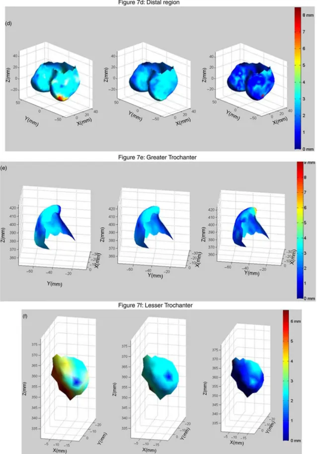
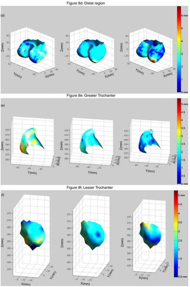
In order to smooth the data and to provide a generic description of the COT distributions, the COT vectors and matrices were averaged over the database. The mean averaged COT for each anatomic region is provided as the first information of difference between the regions. To study the COT distribution within the anatomic regions, a generic 3D mesh of each anatomic region is plotted, enhanced with a colour map representing the COT values, as proposed by Treece et al. (2010) or Poole et al. (2011) for the proximal femur. For the diaphysis and the neck, the COTs are moreover represented as 3D surface maps. The COT distribution along with two slicing planes for the diaphysis, located around 70% (plane A) and 25% (plane B) of the diaphysis height, and one slicing plane for the neck, located at about 66% of the trochanteric-head borders of the neck region, are more precisely described as representative samples of the distribution for the whole structure. They will be referred to as representative planes. In order to study the variability of the COT distribution, a PCA was applied to the 24 COT subvectors of each anatomic region. The two first deformation modes of the PCA were considered and were evaluated in terms of percentage of variance explanation and 2RMS error reconstruction. For each deformation mode, nomograms Figure 2. Three CT scans corresponding to the three planes displayed on the left, superimposed with the contours of the final solution of the internal and external cortical surfaces intersected with the scan planes (plain lines); the contours of the initial solution of the external cortical surface are displayed in dashed lines.

of the COT distributions for each anatomic region are displayed on generic 3D meshes enhanced with colour maps as mentioned above and as COT profiles in the three representative planes. The variations of the mean COT by region according to the two PCA parameters are finally provided.

3. Results

3.1 Accuracy of the reconstruction method and of the COT measurements

The mean, 2RMS and maximum point-to-surface errors of the internal and external cortical surfaces for which Amira reference meshes exist are summarised in Table 1. The

mean and maximum relative volume errors for the same femurs are provided inTable 2.

All the reconstructions were moreover qualitatively checked visually by superimposing on the CT scans the 3D contours of the meshes resulting of the intersections of the CT scans 3D planes and the reconstructed meshes, as visible inFigure 2.

The mean, 2RMS and maximum errors of the COT measured on the surfaces obtained from our reconstruc-tion method to the COT measured on the reference surfaces are summarised by anatomic region for the 10 femurs inTable 3.

3.2 Cortical thickness description 3.2.1 Cortical thickness distribution

The COT averaged on the database as mentioned above is the same as the COT obtained with the parameters of the PCA set to 0. As a consequence, the mean COTs by region are given by the second and fifth columns of Table 5. Table 1. Mean, 2RMS and maximum point-to-surface distances of the surfaces reconstructed with our method to the Amira reference meshes for 10 femurs.

Mean (mm) 2RMS (mm) Maximum (mm) Internal cortical surface 0.5 1.7 6.5 External cortical surface 0.3 1.2 6.4

Table 2. Mean and maximum errors of the volumes of the internal and external cortical surfaces and of the cortical bone reconstructed with our method in reference to the volumes of 10 Amira reference meshes.

Mean (%) Max. (%) Internal cortical surface 3.7 7.8 External cortical surface 2 4.2

Cortical bone 7.8 17.3

Figure 3. 3D surface mesh of a femur with the six anatomic regions of the study in colour: diaphysis in blue, neck in red, head in green, distal region in magenta, greater trochanter in cyan and lesser trochanter in black.

Table 3. Mean, 2RMS and maximum errors of the COT measured on the surfaces obtained from our reconstruction method to the COT measured on the reference surfaces by anatomic region for 10 femurs.

Mean (mm) 2RMS (mm) Maximum (mm) Total 0.8 2.0 7.7 Diaphysis 0.6 1.5 6.7 Neck 0.8 2.1 6.9 Head 1.0 2.3 4.3 Distal region 0.7 1.9 7.7 Greater trochanter 0.8 1.9 4.2 Lesser trochanter 1.0 2.6 6.3

Similarly, the generic 3D mesh of each region enhanced with the colour map representing the averaged COT is visible on the middle ofFigures 7 and 8. For the diaphysis and the neck, the averaged COT maps are additionally displayed in Figure 4. According toTable 5, the average COT is interestingly around 2 mm for all the regions of the femur, except for the diaphysis for which it is 4.8 mm.

The diaphysis COT, as visible inFigure 4(a) and (b), shows linear increase from the diaphysis bottom to about 50 – 60% of its height. It varies then between 4.5 and 7.5 mm until about 85% of the diaphysis height, where it starts decreasing. The COT in the planes perpendicular to the main axis is not equally distributed and the variations for the two representative planes are displayed inFigure 5. The COT in the distal plane B is characterised by a V-shape in

Figure 5(a)corresponding to a higher COT for the posterior diaphysis as schematised on the axial view of the Figure 5(c). The COT in the proximal plane A is characterised by a wavelike shape around the centre of the diaphysis and appears to be very well approximated by a sixth-order polynomial as visible in Figure 5(a). We verified on the whole diaphysis that this order corresponds to the lowest order that reduces significantly the approximation error. As schematised on the axial view ofFigure 5(b), the wavelike shapes correspond to an ellipsoidal distribution, the main axis oriented in the medial – lateral direction with a small posterior protuberance. In other words, we show here that one can approximate the COT distribution in plane A with an ellipsoid having a small protuberance, this geometric figure being the best simple figure, equivalent to a sixth-order polynomial when seen as a profile around its axis. In plane B, the ellipsoid corresponds rather to a circle whose centre is slightly shifted towards the posterior diaphysis.

The neck COT, as visible inFigure 5(c), shows a similar pattern in the planes perpendicular to the main axis from the trochanteric borders towards the head: a lower level and an upper level. The COT distribution in the representative plane is displayed inFigure 6(a)and shows the two levels. This results in a wavelike shape, characterised in the plane view by a circular distribution whose centre has an offset of about 0.5 mm towards the inferior neck (Figure 6(b)), the neck presenting thus bigger COT in the inferior part and smaller COT in the superior part. By analogy with the diaphysis characterisation, we approximated the COT in the representative plane by a third-order polynomial to approach the wavelike shape. We verified on the whole neck that the third order corresponds to the lowest order that reduces significantly the approximation error. As for the diaphysis, it means that one can approximate the neck COT simply as a circle around the main axis whose centre is slightly shifted so as to increase COT in the inferior neck and to decrease it in the superior neck.

The COT distributions of the other anatomic regions are visible in the middle ofFigures 7 and 8. No clear trend could be found which could describe the characteristics of

the COT distributions. For the head, the COTs appear slightly bigger at its basis, in contact with the neck. For the distal region, the COTs appear rather equally distributed on the region, with higher thickness on the two external corners of the condyles, this distribution being, however, possibly an artefact of the segmentation. The greater trochanter presents rather equally distributed COT on its walls with bigger COT on its top. On the contrary, the lesser trochanter presents smaller COT on its top than on its walls.

3.2.2 Cortical thickness variability

The results of the PCA by region are summarised in

Table 4and the variations of the mean COT by region in relation to the PCA parameters in Table 5. The 3D nomograms of the COT of the first and second mode of deformation for the six anatomic regions are visible in

Figures 7 and 8. The nomograms of the COT in the representative planes of the diaphysis and the neck are displayed inFigures 9 and 10.

The PCA results show consistent trends across the six regions. The first deformation mode corresponds primarily to a variation of the mean COT while keeping the distribution rather unchanged. This is particularly visible on the diaphysis for which the COTs are more accurate and bigger than in the other regions, resulting in larger and clearer variations. We can, therefore, observe inFigure 9

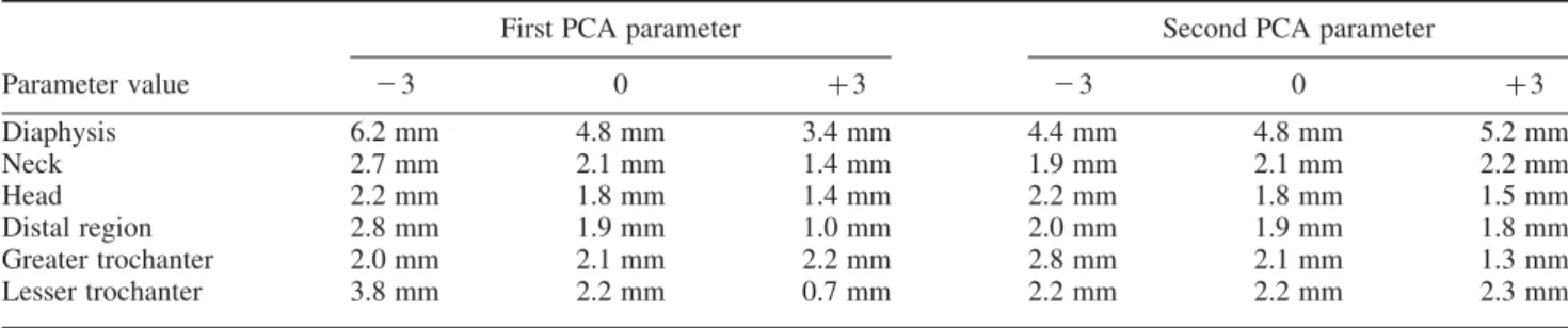
that the COT profiles for the diaphysis never cross each other when the value of the first deformation mode varies: the average COT profiles, plot in bold, keep mainly the same pattern and change mean value. This observation remains true to a lesser extent for the other regions. Indeed, as for the neck, whose COT profile variations in its representative plane are also displayed in Figure 9, the variation around its mean value is also associated with a distribution readjustment corresponding to variability across subjects. The main trend remaining, however, the variation of the mean value of the COT, representing between 16% and 50% of the variance of the COT depending on the region (see Table 4), this effect being represented by the second deformation mode for the greater trochanter. This trend is clearly visible on the variation of the mean COT values inTable 5: the first PCA parameter has a large effect on the mean COT values whereas the second parameter does not, this observation being reversed for the greater trochanter.

As suggested above, the second PCA deformation mode keeps mainly the mean COT unchanged while adjusting the distribution around it, this effect correspond-ing to the first deformation mode for the greater trochanter. The variations are logically smaller in amplitude than for the first deformation mode, counting for 9 – 16% of the variance depending on the region, 28% for the greater trochanter. As illustrated inFigure 8, the COT distribution

Figure 4. Averaged 3D surface map of the COT for the diaphysis (a and b) and the neck (c); the bold lines represent the COT profiles along the representative planes of the diaphysis and the neck, further displayed inFigures 5 and 6; the scale along the axis distal – proximal for subplots (a) and (b) and head – trochanter for subplot (c) is in arbitrary unit between 0 and 1.

changes whereas the mean COT remains rather constant, this effect being characterised in Figure 10 by COT profiles crossing each other around the average COT profile plot in bold. On a more global scale, we can observe in Table 5 that the mean COTs remain rather constant when the second PCA parameter varies.

In summary, the results of the PCA show a clear trend for the variability of the COT of the femur: the first source of variability between the subjects corresponds mainly to the mean thickness of cortical bone, whereas the second is associated with subject-specific distribution around this mean thickness by subject. One can thus approximate the COT of a subject in four steps: (1) setting the COT with a fixed value by region as provided byTable 5, (2) using the

average COT proposed in this study, then (3) adapting the mean COT by anatomic region to the subject character-istics and keeping the distribution unchanged and (4) adapting the COT distribution to the subject characteristics.

4. Discussion

4.1 Protocol, reconstruction method and COT measure This study relates to the COT distribution and variability of the femur, assessed by means of measurements completed on CT data. For technical reasons, it was not possible to dispose of histomorphometry data which provide ground truth for the measurement of cortical bone. The accuracy of Figure 5. COT profiles (plain lines) and COT profiles approximated by sixth-order polynomials (dashed lines) around the diaphysis central axis in the two representative planes of the region (subplot a). Schematic axial representation of the internal and external cortical contours (plain lines) of the diaphysis in each of the two representative planes A and B (subplots b and c); the internal cortical surface is represented by the inner circle of arbitrary radius; the external cortical surface is the inner circle augmented with (1) the best fit of constant thickness over the plane (plain outer circle) or (2) the sixth-order polynomial approximation of the real COT (dashed outer circle) as visible on figure (a).

CT data to measure cortical bone has, however, been assessed in the literature for earlier recording systems (see e.g. Hangartner and Gilsanz 1996; Preidler et al. 1997; Prevrhal et al. 1999). Very good accuracy was reported (Prevrhal et al.1999), although measurement errors of the COT could be up to 10% (Prevrhal et al. 1999) to 15% (Preidler et al.1997). An inherent limitation is the measure of very thin COT. The limit under which the thickness is not measured accurately depends on the properties and experimental set-up of the recording system. As an illustration, Prevrhal et al. (1999) set it at 0.7 mm for a slice thickness of 1 mm and comparable kernel to our study. The more recent scanner and the slice thickness of 0.75 mm should ensure accurate values for most of the COTs measured in this study.

The study relies on the 3D reconstruction of the internal and external cortical surfaces of 24 cadaveric femurs. Considering the difficulty to gather accurate and valid CT scans for such a population, we consider this amount as reasonable, even though it should be expanded in further studies. In terms of comparison, we shall cite the study of Treece et al. (2010), the closest study to this one according to us, based on 18 subjects and limited to proximal femur or the study of Chaibi et al. (2011) based on 31 subjects but limited to external cortical surface extraction.

Our study is, however, limited by the population used to perform our measurements. All the subjects are older than 56 and most of them are males. This limits the generalisation of our study and the variability should be expanded in further studies by having a younger and

more balanced male – female population. The age should especially be considered cautiously in the future as it has an impact on the COT (e.g. Mayhew et al. 2005). Also, an additional limit is the lack of information related to the patients particularly bone status and metabolic data in addition to what was visible on the images. The causes of death were, however, known and were not related to specific pathologies of the locomotor system while no bone metastasis were recorded for the tumorous pathology cases. This lack of information can moreover be balanced by the fact that most of the subjects were males, less exposed to osteoporosis than females. The description provided in this study is, therefore, appropriate for an asymptomatic elderly population, limiting the generalisation. However, if the absolute COT values have to be generalised with caution, the proportion of COT within the femur may remain true for a larger population. In addition, this study constitutes to the best of our knowledge the first description of the distribution and the variability of COT for the femur and can serve as a reference for further developments.

The 3D reconstruction method from CT scans proposed in this study constitutes an innovative alternative to the traditional methods based on manual segmentations on scans. This method takes advantage of the recent developments in 3D reconstruction from biplanar images (Chaibi et al.2011) to provide a fast, robust and accurate initial reconstruction. The method to obtain the accurate 3D internal and external cortical surfaces for the whole femur is then fully automatic. Consequently, after the initialisation which does not take more than 5 min for one Figure 6. COT profile (plain line) and COT profile approximated by a third-order polynomial (dashed line) around the neck central axis in the perpendicular plane of the region (left subplot). Schematic axial representation of the internal and external cortical contours (plain lines) of the neck in the same plane (right subplot); the internal cortical surface is represented by the inner circle of arbitrary radius; the external cortical surface is the inner circle augmented with (1) the best fit of constant thickness over the plane (plain outer circle) or (2) the third-order polynomial approximation of the real COT (dashed outer circle) as visible on the left.

Figure 7. 3D visualisation of the six anatomical regions for the first PCA mode value set at23 (left), 0 (centre) and þ3 (right) enhanced with COT values as colour; the second PCA value remains constant at 0; the neck axis is plotted on (b) and (c) to help interpretation; the bold lines on the 3D meshes in (a) and (b) represent the position of the representative planes of the diaphysis and the neck for which nomograms of the COT profiles for this PCA mode are displayed in Figure 9.

Figure 8. 3D visualisation of the six anatomical regions for the second PCA mode value set at23 (left), 0 (centre) and þ3 (right) enhanced with COT values as colour; the first PCA value remains constant at 0; the neck axis is plotted on (b) and (c) to help interpretation the bold lines on the 3D meshes in (a) and (b) represent the position of the representative planes of the diaphysis and the neck for which nomograms of the COT profiles for this PCA mode are displayed in Figure 10.

femur (Chaibi et al. 2011), no further interaction is required from the operator. In addition, the meshes generated by our method present the advantage to be already divided into anatomic regions and to have all the same topology, which is a strong asset for automatic processing for medical applications. In comparison, Treece et al. (2010) propose a solution for the proximal femur based on manual segmentation of the external cortical surface. As far as we know, the only other fully automatic solution is the one provided by Kang et al. (2003) based on voxel segmentation and tested on the hip and the knee.

The accuracy of our reconstructions was evaluated in reference to 10 pairs of internal and external cortical surfaces segmented manually. The construction of such a reference database required heavy manual work and appeared as relatively complex. The segmentations were carried out by a trained operator and their quality checked visually afterwards by a medical doctor specialised in bone modelling. The external cortical surface segmentation was considered as perfect, whereas more discussions arose about the internal cortical surface segmentation. Indeed, the boundary between cortical and spongy bone seems sometimes hard to define on the CT scans, the grey levels decreasing progressively from the white of the cortical bone towards the grey of the spongy bone without showing a clear step which could mark the boundary. In these cases,

the operator who made the segmentations tended to include some areas as cortical bone which could have been labelled as spongy bone as well. In some regions such as the distal femur, the cortical bone is sometimes so limited that it is almost invisible on the scans and can appears even darker than some parts of the spongy area. These difficulties to segment the internal cortical surface introduces limitations in the accuracy results presented in this study on the internal cortical surface and on the COT. We intended to overcome these limitations by developing a rather large reference database of 10 femurs, i.e. 20 surfaces, which required heavy manual work. We hypothesise, however, that the possible uncertainties of segmentations are rather negligible in comparison to the accuracy results presented in the paper.

Our method has been applied to 28 femurs, and 4 of them have finally been discarded due to segmentation errors in the greater trochanter region (one case) and in the distal region (three cases). The latter errors seem to be a consequence of the difficulty to observe the cortical bone in the distal region, as mentioned above. The 14% failure rate of our method seems, however, reasonable consider-ing the little contribution required by the operator. The method can thus be used in this state as a fast and robust method to obtain segmentations of the internal and external cortical surfaces of the femur from CT scans, only few cases leading to segmentations errors. The frame proposed in this study can also be extended easily to further bony structures with little adaptation.

The reconstructions show volume errors relatively small, in average 2% and 3.7% for the external and internal cortical surfaces. This appears higher than the results below 1% provided by Kang et al. (2003), the comparison remaining, however, difficult as they are the results of a repeatability study computed on a neighbourhood of the neck. The volume of the cortical bone, i.e. the differential volume between the external and the internal surfaces, shows logically a higher error of 7.8% in average. This can be ascribed to the much smaller volume of this structure in comparison to the volume of the two cortical surfaces, which induces higher errors in relative, and to the way to obtain this volume, which accumulates the errors of the two cortical surfaces.

Table 4. Percentage of explained variance and 2RMS reconstruction errors for the two first modes of deformation of the PCA for the six anatomic regions.

Percentage of explained variance 2RMS reconstruction error

PCA deformation mode 1st (%) 2nd (%) 1st (mm) 1st þ 2nd (mm) Diaphysis 39 12 1.4 1.2 Neck 18 13 1.3 1.2 Head 16 16 1.2 1.1 Distal region 29 10 1.4 1.3 Greater trochanter 28 20 1.4 1.2 Lesser trochanter 50 9 1.2 1.1

Table 5. Mean COT values for the six anatomic regions depending on the values of the two parameters of the PCA. First PCA parameter Second PCA parameter

Parameter value 23 0 þ3 23 0 þ3 Diaphysis 6.2 mm 4.8 mm 3.4 mm 4.4 mm 4.8 mm 5.2 mm Neck 2.7 mm 2.1 mm 1.4 mm 1.9 mm 2.1 mm 2.2 mm Head 2.2 mm 1.8 mm 1.4 mm 2.2 mm 1.8 mm 1.5 mm Distal region 2.8 mm 1.9 mm 1.0 mm 2.0 mm 1.9 mm 1.8 mm Greater trochanter 2.0 mm 2.1 mm 2.2 mm 2.8 mm 2.1 mm 1.3 mm Lesser trochanter 3.8 mm 2.2 mm 0.7 mm 2.2 mm 2.2 mm 2.3 mm

In terms of point-to-surface distances, the surfaces appear rather well reconstructed, with a 2RMS error below 2 mm and approaching 1 mm for the external cortical surface, as visible inTable 1. The better reconstruction of the external cortical surface can easily be explained by the clearer borders of the cortical bone with the exterior than with the interior. Beyond the inherent accuracy of the reconstruction method, a part of the error can be ascribed to the smoothness of the reconstructed surface which could not always match the abrupt changes of the targeted structures. The smoothness itself is due either to the postprocessing which consisted in discarding outliers

pinpointed as making sharp tips on the mesh, participating also in smoothing the correct abrupt changes sometimes, either to the relatively low density of the mesh. The latter point could be improved by increasing the density of the mesh, leading however to a longer processing time and possibly higher sensitivity to false detections.

Similarly as for the volume errors, as visible inTable 2, the COT errors come higher than the distance surface errors, cumulating the uncertainties of the two surfaces. Except for the diaphysis at 1.5 mm, the 2RMS errors appear around 2 mm in general and for the whole femur, up to 2.3 and 2.6 mm for the head and the lesser trochanter. In terms Figure 9. Nomograms of the COT profiles for the first mode of deformation of the PCA in the representative planes of the diaphysis and of the neck; variations are equally distributed between the minimum and maximum of the two parameters found in the database, plotted in green and red lines, the average being plotted in bold lines.

Figure 10. Nomograms of the COT profiles for the second mode of deformation of the PCA in the representative planes of the diaphysis and of the neck; variations are equally distributed between the minimum and maximum of the two parameters found in the database, plotted in green and red lines, the average being plotted in bold lines.

of comparison, Treece et al. (2010) attain 2RMS errors of 1.5 mm for the proximal femur once the external cortical surface is known. The smaller errors in the diaphysis can be ascribed to the much clearer cortical boundaries than in the other regions. These accuracy results, although reasonable in general, underline the difficulty of obtaining reliable COT data and warn us to take the results for the head and lesser trochanter with caution.

Overall, for the purpose of COT modelling, one of our aims within this study was to develop a robust and automatic 3D reconstruction method from CT scans able to provide COT on the whole femur. This has been achieved by developing an innovative approach taking advantage of the recent work of Chaibi et al. (2011), requiring extremely limited manual intervention and making our approach an interesting alternative to other approaches proposed in the literature (Kang et al. 2003; Treece et al. 2010). We validated it on a database of 10 femurs for which we obtained manual segmentations as reference. It applies to the whole femur, and the method can interestingly be extended to other bony structures with limited adaptation.

Several points could be improved to enhance the accuracy. First, the accuracy relies on the accuracy of the initial solution provided by Chaibi et al. (2011). Increasing the accuracy of this initial solution could increase the robustness and convergence of the process and could allow the development of more local and accurate techniques. As emphasised by Treece et al. (2010), taking into account both models of the object being scanned and of the image formation process should also provide interesting inputs towards better detection of the cortical bone. Another way to improve accuracy would also be to enhance the signal-to-noise ratio of the CT scans and to apply image processing routines in the planar images to match more precisely our solution to the targeted structures.

4.2 Cortical thickness distribution and variability As generic distribution, we have chosen to represent the averaged COT distribution computed for all the 24 subjects of our study. Limit and advantage of our study, the relatively aged population ensures a rather homo-geneous age (10 years of age standard deviation), justifying the averaging. One can object that such a process hides individual characteristics, but our motivation was to provide a first description of the COT distribution for the femur, not detailed in the literature so far, which could help understanding and modelling the cortical bone. Also, we have complemented this study by a variability study to highlight the main trends of differentiation of the population around the averaged distribution. The two stages of the study have thus to be regarded as complementary for COT analysis.

We have chosen to represent 3D meshes augmented with COT information as proposed by Treece et al. (2010)

or Poole et al. (2011) and additionally 3D surface maps of COT when it was possible, i.e. for the diaphysis and the neck. This has been driven by our motivation to provide a parametric analysis of the COT distribution and to characterise the variability of this distribution. The cylindrical shapes of the neck and the diaphysis allowed an easy surface map projection and shape analysis. On the contrary, the projection of the COT of the other regions on a surface map turned to be more difficult, and we finally decided not to perform it as it increases complexity while providing limited interpretation gain.

COT measurements can vary depending on the calculation vector orientation. Thickness can be defined along vectors perpendicular to the structure to measure. However, arbitrary choices have to be made when the external and internal cortical surfaces are not strictly parallels. This can lead to artificially high COT values to be ascribed to the measurement technique. We have chosen in our study to rely on the geometric properties of the external cortical surface to define COT measurement orientation. This has been motivated by the better accuracy of the external mesh and its available regionalisation as proposed by Chaibi et al. (2011). Artefacts have, however, been observed at the borders of this regions, such as the trochanter – neck border, the lower side of the head, the distal side of the diaphysis or the borders of the distal region. These artefacts remains, however, limited and we hypothesise that they do not alter the general distribution and variability of the COT.

The diaphysis COT is characterised by a rather circular distribution in the distal region, with an offset slightly posterior, whereas rather ellipsoidal in the proximal region, with thinner medial and lateral walls (see Figure 5). In general, the proximal region presents thicker cortical structure than the distal region. These results are in general good agreement with those of Stephenson and Seedhom (1999) who found smaller COT in the distal diaphysis and anterior COT smaller than the medial, lateral and posterior COT along the whole diaphysis. The neck COT distribution keeps the same pattern from the trochanteric border towards the head border and is characterised by a smaller COT for the superior neck and a bigger COT for the inferior neck (seeFigures 4(c) and 6). The results on the neck COT distribution are in general good agreement with the distributions provided by Treece et al. (2010) and Poole et al. (2011) and the results of Mayhew et al. (2005) who found a thicker inferior cortical bone.

The head as visible in the middle of Figures 7 and 8

presents a rather homogeneous COT over its whole surface. It appears slightly different from the distributions provided by Treece et al. (2010) for which the basis of the head in contact with the neck shows thinner cortical bone than the rest of the region. The greater and lesser trochanter, also visible in the middle of the same figures, present, respectively, bigger and smaller COT on their

summit, as opposed to the distributions provided by Treece et al. (2010) for the lesser trochanter. The higher COT errors for this latter region lead us, however, to consider these results with caution. As far as we know, the COT distributions provided for the distal region are original and could not be compared to literature results. The spots of bigger COT on the lower external corners of the condyles can rather be ascribed to reconstruction artefacts.

Global COT distributions are also provided by region inTable 5. Such types of results had never been presented in the literature and provide interesting inputs. Indeed, the average COT of each region is measured at about 2 mm, except for the diaphysis at 4.8 mm. Of course these averaged COT hide variations within each region as detailed above, but it provides a first and global estimate of the COT by region.

The PCA results provided in this study show consistent trends for the two first deformation modes across the four anatomic regions. More precisely, we observe that the variations of the COT profiles for the first deformation mode consist mainly in changing the mean value of the profile while keeping its shape pattern unchanged. On the contrary, the variations related to the second deformation modes, much lower in amplitude than the first mode, are mainly related to shape deformations while keeping the mean value unchanged.

These results draw the outlines of possible modelling of the COT in a near future. Four levels of COT modelling for a specified subject can be, for example considered, each of them being more accurate than the previous level: (1) the COT of each vertex can simply be set at the mean COT value of its region, provided in Table 5; (2) the COT distribution can be chosen as the averaged COT distribution computed across the database; (3) the COT distribution of the previous level can be kept, the mean value of each region being adapted for the considered subject (corre-sponding to the first PCA mode of the study) and (4) the COT distribution shape per se is adapted to the considered subject while keeping the mean COT unchanged (corre-sponding to the first PCA mode of the study). Although the accuracy of the COT estimation increases evidently with the level of modelling, the appropriate level can be determined according to the requirements. As an illustration, the algorithm requiring the calculation of virtual X-rays for automatic determination of femur condyle on biplanar X-rays (Serrurier et al.2012) shows good results with a level 2 modelling. In other words, the results obtained in this study constitute a first step towards the personalisation of the femur COT of a subject while reconstructing its 3D surface from biplanar X-rays. As mentioned in Section 1, this personalisation opens large perspectives, both for research and medical purpose.

5. Conclusion

The objective of this study was the description of the distribution and variability of the COT for the whole femur for asymptomatic subjects, which had never been detailed in the literature. For that purpose, we have developed an original 3D reconstruction method for both internal and external cortical surfaces of the femur from CT scans with very limited interaction with the operator. This method provides meshes with similar topology and divided into anatomic regions. We have reconstructed a database of 28 pairs of internal and external cortical surfaces of the full femurs by means of our technique and extracted their COT. The reconstructions showed a good accuracy to the manual reconstructions in overall, despite the more difficult reconstructions of the proximal and distal femur. A description of the COT distribution has been provided for the diaphysis, the neck, the head, the distal femur and the lesser and greater trochanters. The correlations were analysed by means of PCA. It revealed that the first source of variability across our population was the mean value of the COT for each anatomic region, while the distribution variability appeared only in second rank (except for the greater trochanter). These results draw the outlines for personalised modelling of the COT from biplanar X-rays in the clinical routine. A large range of medical applications can be expected from such modelling in the future, such as personalised mechanical simulations and risk fracture prediction or personalised hip design. A first application of these results has been developed by Serrurier et al. (2012) for more automation in the 3D femur reconstruction from biplanar X-rays.

Acknowledgements

This work is part of the SterEOS þ project funded by the Ile-de-France region though the Medicen competitive cluster. The authors would like to thank the donors, the ‘Service du don des corps’ of the University Paris Descartes, for providing the PMHS, the Radiology Service of Cochin University Hospital for the CT-Scan, the CEESAR and the LAB (GIE PSA Renault) for the technical support. The study benefited also of useful discussions with Benjamin Aubert and manual segmentations completed by Hussam Hanna. Finally, we would like to thank two anonymous reviewers who helped us to improve the paper.

References

Adam F, Hammer D, Pape D, Kohn D. 2002. Femoral anatomy, computed tomography and computer-aided design of prosthetic implants. Arch Orthop Trauma Surg. 122:262 – 268.

Barnett E, Nordin B. 1960. The radiological diagnosis of osteoporosis: a new approach. Clin Radiol. 11(3):166 – 174. Bousson V, Le Bras A, Roqueplan F, Kang Y, Mitton D, Kolta S,

Bergot C, Skalli W, Vicaut E, Kalender W, Engelke K, Laredo JD. 2006. Volumetric quantitative computed tomogra-phy of the proximal femur: relationships linking geometric and

densitometric variables to bone strength. Role for compact bone. Osteoporosis Int. 17:855–864.

Bra˚ten M, Nordby A, Terjesen T, Rossvoll I. 1992. Bone loss after locked intramedullary nailing. Acta Orthop. 63(3): 310 – 314.

Chaibi Y. 2010. Adaptation des me´thodes de reconstruction 3D rapides par ste´re´oradiographie: mode´lisation du membre infe´rieur et calcul des indices cliniques en pre´sence de de´formation structurale.

Chaibi Y, Cresson T, Aubert B, Hausselle J, Neyret P, Hauger O, de Guise JA, Skalli W. 2011. Fast 3D reconstruction of the lower limb using a parametric model and statistical inferences and clinical measurements calculation from biplanar X-rays. Comput Methods Biomech Biomed Eng. 1:1.

Chan AH, Crowder CM, Rogers TL. 2007. Variation in cortical bone histology within the human femur and its impact on estimating age at death. Am J Phys Anthropol. 132(1):80 – 88.

Croker SL, Clement JG, Donlon D. 2009. A comparison of cortical bone thickness in the femoral midshaft of humans and two non-human mammals. HOMO J Comp Hum Biol. 60(6):551 – 565.

de Bruin PW, Kaptein BL, de Bruin PW, Kaptein BL, Stoel BC, Reiber JH, Rozing PM, Valstar ER. 2008. Image-based RSA: roentgen stereophotogrammetric analysis based on 2D-3D image registration. J Biomech. 41(1):155 – 164.

Fokapu O, Girard J.-P. 1993. ECG time and frequency evolution: beat to beat analysis [French]. Innov Tech Biol Med. 14(1):102 – 112.

Hangartner TN, Gilsanz V. 1996. Evaluation of cortical bone by computed tomography. J Bone Mineral Res. 11(10):1518 – 1525.

Ho¨gler W, Blimkie CJ, Cowell CT, Kemp AF, Briody J, Wiebe P, Farpour-Lambert N, Duncan CS, Woodhead HJ. 2003. A comparison of bone geometry and cortical density at the mid-femur between prepuberty and young adulthood using magnetic resonance imaging. Bone. 33(5):771 – 778. Humbert L, De Guise JA, Aubert B, Godbout B, Skalli W. 2009.

3D reconstruction of the spine from biplanar X-rays using parametric models based on transversal and longitudinal inferences. Med Eng Phys. 31(6):681 – 687.

Jolivet E, Sandoz B, Laporte S, Mitton D, Skalli W. 2010. Fast 3D reconstruction of the rib cage from biplanar radiographs. Med Biol Eng Comput. 48(8):821 – 828.

Kang Y, Engelke K, Kalender WA. 2003. A new accurate and precise 3-D segmentation method for skeletal structures in volumetric CT data. IEEE Trans Med Imaging. 22(5):586 – 598.

Laine H-J, Kontola K, Lehto MU, Pitka¨nen M, Jarske P, Lindholm TS. 1997. Image processing for femoral endosteal anatomy detection: description and testing of a computed tomography based program. Phys Med Biol. 42(4):673. Laporte S, Skalli W, de Guise JA, Lavaste F, Mitton D. 2003. A

biplanar reconstruction method based on 2D and 3D contours: application to the distal femur. Comput Methods Biomech Biomed Eng. 6(1):1 – 6.

Mayhew PM, Thomas CD, Clement JG, Loveridge N, Beck TJ, Bonfield W, Burgoyne CJ, Reeve J. 2005. Relation between

age, femoral neck cortical stability, and hip fracture risk. Lancet. 366(9480):129 – 135.

Noble PC, Alexander JW, Lindahl LJ, Yew DT, Granberry WM, Tullos HS. 1988. The anatomic basis of femoral component design. Clin Orthop Relat Res. 235:148 – 165.

Noble PC, Box GG, Kamaric E, Fink MJ, Alexander JW, Tullos HS. 1995. The effect of aging on the shape of the proximal femur. Clin Orthop Relat Res. 316:31 – 44.

Pan J, Tompkins WJ. 1985. A real-time QRS detection algorithm. IEEE Trans Biomed Eng. 32(3):230 – 236.

Poole KES, Treece GM, Ridgway GR, Mayhew PM, Borggrefe J, Gee AH. 2011. Targeted regeneration of bone in the osteoporotic human femur. PLoS ONE. 6(1):e16190.

Preidler KW, Brossmann J, Daenen B, Pedowitz R, De Maeseneer M, Trudell D, Resnick D. 1997. Measurements of cortical thickness in experimentally created endosteal bone lesions: a comparison of radiography, CT, MR imaging, and anatomic sections. Am J Roentgenol. 168(6):1501 – 1505.

Prevrhal S, Engelke K, Kalender WA. 1999. Accuracy limits for the determination of cortical width and density: the influence of object size and CT imaging parameters. Phys Med Biol. 44(3):751.

Robertson DD, Walker PS, Granholm JW, Nelson PC, Weiss PJ, Fishman EK, Magid D. 1987. Design of custom hip stem prostheses using three-dimensional CT modeling. J Comput Assist Tomogr. 11(5):804 – 849.

Seebeck J, Goldhahn J, Sta¨dele H, Messmer P, Morlock MM, Schneider E. 2004. Effect of cortical thickness and cancellous bone density on the holding strength of internal fixator screws. J Orthop Res. 22(6):1237 – 1242.

Serrurier A, Quijano S, Nizard R, Skalli W. 2012. Robust femur condyle disambiguation on biplanar X-rays. Med Eng Phys., in press.

Smith HW, De Smet AA, Levne E. 1982. Measurement of cortical thickness in a human cadaver femur. Conventional roentgenography versus computed tomography. Clin Orthop Relat Res. 169:269 – 274.

Stephenson P, Seedhom BB. 1999. Cross-sectional geometry of the human femur in the mid-third region. Proc Inst Mech Eng H. 213(2):159 – 166.

Sugano N, Ohzono K, Nishii T, Haraguchi K, Sakai T, Ochi T. 1998. Computed-tomography-based computer preoperative planning for total hip arthroplasty. Comput Aided Surg. 3(6):320 – 324.

Treece GM, Gee AH, Mayhew PM, Poole KE. 2010. High resolution cortical bone thickness measurement from clinical CT data. Med Image Anal. 14(3):276 – 290.

Trochu F. 1993. A contouring program based on dual kriging interpolation. Eng Comput. 9(3):160 – 177.

Virtama P, Telkka A. 1962. Cortical thickness as an estimate of mineral content of human humerus and femur. Br J Radiol. 35:632 – 633.

Zheng G, Gollmer S, Schumann S, Dong X, Feilkas T, Gonza´lez Ballester MA. 2009. A 2D/3D correspondence building method for reconstruction of a patient-specific 3D bone surface model using point distribution models and calibrated X-ray images. Med Image Anal. 13(6):883 – 899.

Powered by TCPDF (www.tcpdf.org) Powered by TCPDF (www.tcpdf.org) Powered by TCPDF (www.tcpdf.org) Powered by TCPDF (www.tcpdf.org) Powered by TCPDF (www.tcpdf.org) Powered by TCPDF (www.tcpdf.org) Powered by TCPDF (www.tcpdf.org) Powered by TCPDF (www.tcpdf.org) Powered by TCPDF (www.tcpdf.org) Powered by TCPDF (www.tcpdf.org) Powered by TCPDF (www.tcpdf.org) Powered by TCPDF (www.tcpdf.org) Powered by TCPDF (www.tcpdf.org) Powered by TCPDF (www.tcpdf.org) Powered by TCPDF (www.tcpdf.org) Powered by TCPDF (www.tcpdf.org) Powered by TCPDF (www.tcpdf.org) Powered by TCPDF (www.tcpdf.org) Powered by TCPDF (www.tcpdf.org) Powered by TCPDF (www.tcpdf.org) Powered by TCPDF (www.tcpdf.org) Powered by TCPDF (www.tcpdf.org)