Predictive elution window stretching and shifting as a generic search strategy for automated method development for liquid chromatography

Predictive Elution Window Stretching and Shifting as a Generic

Search Strategy for Automated Method Development for Liquid

Chromatography

Eva Tyteca,

†

Anuschka Liekens,

†

David Clicq,

‡

Ameriga Fanigliulo,

§

Benjamin Debrus,

∥

Serge Rudaz,

∥

Davy Guillarme,

∥

and Gert Desmet*

,†

†_{Vrije Universiteit Brussel, Department of Chemical Engineering (CHIS-IR), Pleinlaan 2, 1050 Brussels, Belgium} ‡_{UCB Pharma, Analytical Development Chemicals, Chemin du Foriest, 1420 Braine L'alleud, Belgium}

§_{Aptuit, via Fleming 4, 37135 Verona, Italy}

∥_{University of Geneva, University of Lausanne, School of Pharmaceutical Sciences, Boulevard d'Yvoy 20, 1211 Geneva 4, Switzerland}

*

S Supporting Information

ABSTRACT: We report on the possibilities of a new method development (MD) algorithm that searches the chromato-graphic parameter space by systematically shifting and stretching the elution window over different parts of the time-axis. In this way, the search automatically focuses on the most promising areas of the solution space. Since only the retention properties of thefirst and last eluting compounds of the sample need to be (approximately) known, the algorithm can be directly applied to samples with unknown composition, and the proposed solutions are not sensitive to any modeling

errors. The search efficiency of the algorithm has been evaluated on an extensive set of random-generated in silico samples covering a broad range of different retention properties. Compared to a pure grid-based search, the algorithm could reduce the number of missed components by 50% and more. The algorithm has also been applied to solve three different real-world separation problems from the pharmaceutical industry. All problems could be successfully solved in a very short time (order of 12 h of instrument time).

O

ne of the most time-consuming tasks in analytical liquid chromatography is method development (MD). This is the search for the chromatographic operating conditions (type of organic modifier and stationary phase, temperature, gradient profile, pH, ionic strength, etc.) leading to the complete resolution of the sample in all its individual constituents.1−9 Because of the high probability for peak overlap10 and the sensitive dependency of the retention time of the individual analytes on, for example, the employed gradient slope, the MD process still involves a lot of trial and error and can take up to several weeks of work.

To speed up this work, fully or semiautomated MD software has been developed over the years.10−16 Roughly spoken, the automated MD strategies described in literature are either search-based (e.g., using the Simplex method)17 or model-based (e.g., Drylab,18Chromsword).19In the present study, the properties of a hybrid method, further referred to as the predictive elution window stretching and shifting method (PEWS2), were investigated. This method explores the chromatographic parameter space in a pure search-mode but also uses the information on the retention properties of some of the peaks (e.g., thefirst and the last peak of the chromatogram and/or thefirst and last peaks of its most problematic zone). This information is used to make a model-based prediction of

the gradient slope (expressed here asβt0= (ϕe− ϕ0)·t0/tG) and

initial gradient compositionϕ₀values that should be imposed to shift and stretch the elution window of the sample in a controlled manner over different parts of the time-axis. Hence, instead of optimizing the gradient by searching in the (ϕ₀,βt₀ )-space, the PEWS2-method searches directly in the (kfirst,klast

)-space. Since the values of k_firstand k_lastdirectly determine how wide the elution window is and whether the components elute early or late, these parameters control the peak capacity and selectivity of the chromatogram in a much more direct way than theϕ0andβt0parameters.

To test the PEWS2-method, it has been applied to a number of different pharmaceutical MD problems. To generalize the results, the search efficiency of the PEWS2-method has also been evaluated in a comprehensive numerical test, involving hundreds of different random in-silico samples with widely differing retention properties. In this numerical part of the study, the PEWS2_{-method is compared to that of a direct search}

in the (ϕ0,βt0)-space using the most simple of all possible Received: May 31, 2012

Accepted: August 19, 2012 Published: August 20, 2012

search algorithms, i.e., using a simple grid search. The latter was selected to minimize the influence of the employed search algorithm itself. In a next step, the PEWS2_{-method can be}

extended with more advanced search methods, for example, by making use of the information on the local slope of the chromatographic response surface. The method can potentially also be applied to enhance the optimization of multisegment gradients.20−23

All searches conducted in the present study were guided using a so-called chromatographic response function or CRF.12,16,20,24−30 The CRF used in the present study was defined as the sum (np*) of the number of observed peaks (np)

and peak shoulders (n_s) plus a so-called noninteger part (NIP), describing the quality of the separation:

* = + + np np ns NIP (1) = Π + Σ a f g bn with NIP i i i i f g crit n i i crit (2)

In this expression, f_i/g_i is the ratio between the depth of the valley fiand the interpolated peak height giand therefore only

varies between 0 and 1,26whereas n_critis the number of critical pairs (i.e., the number of peak pairs for which fi/gi< 1). When a

shoulder is detected, it is counted as an extra peak with an f_i/g_i -value of 0.01. By choosing the -value of the weighing factors a and b such that their sum maximally equals 0.99, the NIP-part can also never exceed this value (NIP ≤ 0.99) because the factors appearing in the two terms have been normalized by respectively taking the (ncrit)throot and by dividing by ncrit. This

implies that conditions revealing a new compound automati-cally get a higher np*-value than conditions leading to a fully

baseline resolved separation but revealing one peak less. In the present study, the values of a and b were taken equal (with a + b = 0.99), but many different variants can be proposed (for example, by taking a = 0, b = 1 or vice versa).

■

EXPERIMENTAL AND NUMERICAL METHODS Numerical Methods. Chromatogram Simulation. All numerical simulations were conducted assuming that the elution properties of the compounds can be described by the linear solvent strength (LSS)-model.31−33This was purely done for the sake of simplicity, since there is no reason to assume that the main conclusions of the present study would be different under non-LSS conditions.

In the LSS-model, the retention properties of a compound are fully described by a kw- and S-value. To simulate a

chromatogram containing n_c compounds, a random number generator was used to randomly pick nc combinations of kw

-and S-values taken from a given interval. Also the injected concentration of each component was randomly picked from a prescribed interval. The reader is referred to Table S1 in the Supporting Information for a list of the employed intervals.

These values, together with a given value of the column efficiency N and the gradient parameters ϕ0 (initial mobile

phase concentration) and βt₀ (gradient steepness β = (ϕ_e − ϕ0)·t0/tG) were subsequently used in a computer program

written in Matlab to simulate the expected chromatograms. Again for the sake of simplicity, the concentration profiles of the different analyte peaks were assumed to be purely Gaussian, such that their variation with the time t can be written as34,35

π = + − − − + = ⎛ ⎝ ⎜ ⎞ ⎠ ⎟ ⎛ ⎝ ⎜ ⎜ ⎜⎜ ⎞ ⎠ ⎟ ⎟ ⎟⎟

(

)

c t t c N k G N k k G c M V (1 ) exp 1 2(1 ) with 2 t t 0 0 e 2 e 2 2 0 0 0 (3)

where t is the time (min), t0the column dead time (min), c0the

injected concentration (g/mL), k_e the retention factor experienced by a compound at the end of the column, k the effective retention factor of a compound (k is given by k = t_R− t0/t0wherein tRis the retention time of the compound), G the

gradient compression factor,36M the injected mass (g), and V₀ the column dead volume (mL).

With the known values of k_w and S, the values of k_e and k have been calculated for each compound as a function of ϕ0

and βt₀ using the expressions proposed by Schoenmakers et al.33

Actual Search Algorithm. The actual search algorithm starts by determining the retention parameters of two (or more) of the most easily identifiable or problematic peaks in the chromatogram. These can be any of the peaks, but for the sake of argument and as an illustrative example, most of the examples in the present study focus on the first and the last peak of the chromatogram. The retention parameters were determined using the measured retention factor k of the peaks of interest and solving the well-established LSS-expressions for k33using the known valuesβt0andϕ0via the Solver-routine in

MS Excel: Regime 1: < < + t₀ t_R t₀ t_D = k_effective k₀ (4a) Regime 2: + < < + + t₀ t_D t_R t₀ t_D t_G = + − + ⎛ ⎝ ⎜⎜⎛_⎝⎜ ⎞ ⎠ ⎟ ⎞ ⎠ ⎟⎟ k t t b t t k b t k 1 ln 1 effective D 0 0 D 0 0 0 (4b) Regime 3: > + + t_R t₀ t_D t_G φ = − + + + − = − ⎛ ⎝ ⎜⎜ ⎛_⎝⎜ ⎞ ⎠ ⎟⎞ ⎠ ⎟⎟ k k k k t t t t t k k b b t t k k S 1 1 exp where exp( ) effective e e 0 D 0 D G 0 e 0 G 0 e w e (4c)

Equations 4a−4c are written in such a way that they take the effect of the system dwell time tD into account. The k-values

were measured for two different values of t_G (and/or ϕ₀) in order to obtain a closed set of two unknowns and two equations (the two measured k-values).

Subsequently, the known values of S and kw are used to

resolve eqs 4a−4c to find the t_G- (incorporated inβt₀) andϕ₀ -values needed to put the peaks of interest as close as possible to the target k-values. In the algorithm, these target values are selected such that they cover the entire solution space as broadly as possible (cf. the black stars in Figure 1b as an example wherein 13 different couples of desired k-values for the

first and last peak in the chromatogram were selected). Typically, the Excel solverfinds a solution in less than 1 min. After the execution of the runs corresponding to each of the different target value combinations (cf. again the 13 black star data points in Figure 1b), the separation quality of each of the obtained chromatograms is calculated using the

CRF-expression given by eqs 1 and 2. Subsequently, some additional fine-tuning runs are conducted around the k-values of the runs with the highest CRF.

Columns, Reagents, and Instruments. Samples. The PEWS2_{-method has also been tested by applying it to a number}

of real-world MD problems. The first sample consisted of an antiepileptic drug (API) and its 13 impurities. The different compounds were diluted in 90/10 H2O/MeOH to a

concentration 1 mg/mL (API) and 0.2 mg/mL (9 impurities). To develop a method with Drylab (Molnár Institute, Berlin, Germany), the different compounds have also been prepared separately. A second mixture, containing four additional impurities, has been included with a concentration of 200 mg/mL. The injection volume was 2 μL, and the detection wavelength was 258 nm.

In a second example, a method was developed for the separation of a new drug under development (API) and its 13 impurities (synthesis intermediates, synthesis side-products, and degradation impurities). The compounds had a MW between 131 and 335 Da with varying polarity due to different functional groups. The sample was dissolved in 50/50 H₂O/ ACN + 0.05% TFA. The injection volume was 20 μL. UV detection was carried out at 275 nm.

In a third example, a method has been developed for a 16 antipsychotic drugs sample, consisting of Maprotiline, Dulox-etine, Chlorpromazine·HCl, Levomepromazine, Clotiapine·-base, Thioridazine, Fluphenazine·2HCl, Aripiprazole, Quetia-pine, fumarate, OlanzaQuetia-pine, Chlorprothixen·HCl, Clozapine, Pipamperone, Brotizolam, Flupentixol·2HCl (both E and Z isomer). These were dissolved in 70/30 H2O/MeOH to afinal

total concentration ranging between 10 and 40 ppm for all the individual compounds. The injected sample volume was equal to 2μL. UV-detection occurred at a wavelength of 230 nm.

Instruments and Columns. For the separation of the antieliptic drug and its impurities, a binary Waters UPLC system (with a dwell volume of 120μL) has been used. Two Waters Acquity HSS columns (2.1 mm × 100 mm, 1.8 μm) have been used for the screening: a T3 and a PFP column. The column temperature was set at 30°C. The mobile phases were H2O + 0.1% TFA and ACN + 0.1% TFA, at aflow rate of 0.400

mL/min.

The separation of the 13 components mixture was done on an Agilent 1100 instrument (with a dwell volume of 1.15 mL). An Achrom ACE 3 C18 AR column (150 mm× 4.6 mm, 3 μm) was used at 40 °C. The two mobile phases used for the gradient elution were an aqueous buffer (ammonium acetate 20 mM pH 5.5) and ACN. Theflow rate was 1 mL/min.

The 16 antipsychotic drugs sample was separated on an Acquity UPLC H-Class instrument (with a dwell volume of 370 μL). Four Waters Acquity columns (50 mm × 2.1 mm 1.7 μm) have been used for the screening: BEH C18, BEH Shield RP18, CSH Fluoro-Phenyl, and BEH Phenyl. The mobile phases were an aqueous buffer (ammonium formate or acetate 20 mM at pH 3, 5, and 9) and ACN. Theflow rate was 500 μL/min, and the columns were operated at a temperature of 45°C.

■

RESULTS AND DISCUSSION

Illustrative Example (Numerical Simulation). A large part of the development and the optimization of the PEWS2 -method was done using simulated chromatograms. A simulation study has the advantage that a large number of cases can be tested in a short time and that the k_w- and S-values of the individual compounds are always exactly known. As a

Figure 1. (a) Example of the (ϕ0,βt0)-contour plot and runs considered in the (ϕ0,βt0)-grid search for one of the considered 15 component samples. (b) Corresponding (k′first,k′last)-contour plot and runs proposed by the PEWS2_{-method. (c) Same runs as in part b but} now represented in the (ϕ0,βt0)-space. Legend:∗, initial search; red ∗, fine-tuning steps.

consequence, it can also be exactly calculated how the optimization goal (i.e., the separation quality number np*)

varies as a function of the chromatographic variablesϕ0andβt0.

In the present study, this information has been used to visualize the efficacy of the PEWS2-method by plotting its search steps against a background formed by a high-resolution contour plot of the value of the optimization goal np*.

Figure 1a shows an example of such a contour plot (n_p* versusφ0andβt0) for the case of a 15 compound mixture. The

brown region in the contour map corresponds to the case with the highest separation resolution. The black star data points represent the search grid used for the pure grid-based search in the (ϕ₀,βt₀)-space. The number of data points (15) was more or less arbitrarily selected for its ability to cover the space in a sufficiently uniform and dense way without needing an excessive amount of runs (assuming a 30 min run time including column regeneration, these 15 runs can be completed in 15× 30 min = 7.5 h of separation run time). The data points at the extremities were left out of the grid search, as these conditions are seldom of importance in reality either.

Figure 1b shows the np*-contour plot of the same sample but

now in a coordinate system formed by the retention coefficient of the first and the last eluting compound (y- and x-axis, respectively). Important to note is that the new search grid (black star data points) is now directly fitted onto the (kfirst,klast)-domain. Since these grid points correspond to a

controlled shifting and stretching of the elution window, they directly represent the physical meaning of the PEWS2-method. To conduct the search, the linear gradient parameters (φ₀ andβt0) corresponding to each of the black star data points in

the (k_first,k_last)-domain are calculated using the k_w- and S-values of the first and last eluting compound collected during two initial scouting runs with different values for tG and running

between 5 and 95% of organic modifier and feeding these data to the well-established LSS-model equations for the effective retention coefficient31and use an iterative search algorithm to find the βt0andϕ0-values yielding the best agreement with the

(kfirst,klast)-combination of the grid point under consideration.

In some cases, the kfirst- and klast-values of the obtained

chromatogram deviated significantly from the expected value. This occurred when the identity of the peaks elutingfirst and or last changed from one (ϕ0,βt0)-combination to another. To

tackle this problem, a limited “peak tracking” strategy was implemented wherein the kw- and S-parameters of the three

first and the three last eluting compounds were continuously updated by scanning through all possible elution order combinations and taking the one that is most consistent with the observed elution pattern. In the very limited number of cases, wherein also this peak tracking failed, the algorithm still returned a very useful set ofβt₀and ϕ₀-conditions. Although leading to a wrong value for kfirst and klast, the resulting

chromatograms contained useful information to proceed with the search.

To illustrate the efficacy of the PEWS2-method, Figure 1c shows the position of the runs proposed by the PEWS2

-algorithm but now plotted in the (ϕ0,βt0)-space. As can be

noted, these runs are much better concentrated around the area(s) of maximal resolution than the runs corresponding to the (ϕ0,βt0)-grid search considered in Figure 1a.

As a consequence, also the additional refinement runs (represented by the pink stars, configured in a square around the two bestfirst round runs in either the (ϕ₀,βt₀)-space or the (kfirst,klast)-space) are much better targeted toward the optimal

solution region in the PEWS2_{-method (Figure 1b,c) than in the}

(ϕ0,βt0)-grid search. Obviously, in the present example, the

search in the (ϕ₀,βt₀)-domain also yielded a good solution (see pink grid point close to the contour plot maximum in Figure 1a). However, the probability that this solution was found is clearly much smaller than for the search in the (kfirst,klast)-space,

where the number of runs proposed by the algorithm close to the contour plot maximum is much larger, as in total 9 of the proposed runs are conducted in the (brown) region of maximal separation resolution. The high number of runs conducted there also provides important information concerning the robustness of the final method. A second example of a fine search is shown in the Supporting Information (Figure S-1).

Comprehensive Numerical Comparison Test. To quantify the potential advantage of the PEWS2_{-method for a}

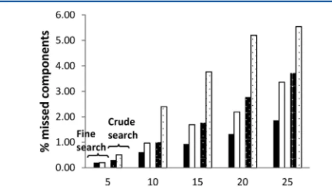
statistically relevant number of samples of different complexity, the method as described in Illustrative Example (Numerical Simulation) has been applied to a large number of in silico samples. Five sample categories were considered, respectively, containing 5, 10, 15, 20, and 25 components. For each category, 200 different samples were generated using the random number generator to pick the kw- and S-values from the different

considered allowable intervals (see Table S-1 in the Supporting Information). For each sample, afine and a crude grid search were conducted. The fine search consisted of 15 initial runs, followed by 2× 4 refinement runs (conducted around the two best solutions obtained in the initial round). The crude search only consisted of 7 initial runs. No additional refinement runs were performed. Two examples of a crude search are shown in the Supporting Information (Figures S-2 and S-3).

Figure 2 compares the number of missed components. As can be noted, the PEWS2-method consistently leads to a

smaller percentage of missed components. The higher the number of compounds per sample, i.e., the more demanding the separation, the larger the gain margin of the PEWS2 -method with respect to the pure (ϕ₀,βt₀)-grid search. This is in agreement with the intuitive expectation that the extra modeling information (i.e., the knowledge of the retention behavior of thefirst and last eluting compounds) builds into the PEWS2_{-method and becomes more useful when the search is}

more difficult. The latter can also be noted by comparing the results of thefine grid search with that of the crude grid search. The latter search conditions are more demanding, explaining

Figure 2.Side-by-side comparison of the PEWS2_{-method (black for} fine search; black with white dots for crude search) and the (ϕ0,βt0 )-grid search (white for fine search; white with black dots for crude search) of the number of missed components of the best separations obtained for each of the 200 considered samples considered per sample difficulty (represented by the different number of compounds contained within them: 5, 10, 15, 20, and 25).

why the advantage of the PEWS2_{-method is more pronounced}

than in thefine grid search case. The fact that it performs so well in a crude grid search suggests that the PEWS2_{method is}

especially suited to efficiently make a first rapid selection when a large number of different combinations of stationary phase, organic modifier, pH, and temperature need to be scouted. Similar conclusions can be made when looking at the average value of the quality criterion np* of the best solution found by

the search algorithms (Figure S-4 in the Supporting Information). Changing the number of assumed theoretical plates from N = 20 000 to smaller (N = 5 000 and 10 000) or larger (N = 40 000) did not change the relative success rate of the two methods.

Overall, it can be concluded that the advantage of the PEWS2-method is that it automatically zooms in on the most promising areas in the search space. This is illustrated in Figure 3, where a side-by-side comparison is made of the n_p*-contour plots in the (ϕ₀,βt₀)-domain and those in the (k_first,k_last)-domain for two (randomly selected) different 15 component samples. Some other examples with varying sample complexity (10, 20, and 25 components) are given in Figure S-5 in the Supporting Information. In each case, the areas corresponding to the

highest separation quality are enlarged when going from the (ϕ₀,βt₀)-domain to the (k_first,k_last)-domain.

Some Real-Life Examples. Separation of an Antiepilep-tic Drug and Its Impurities. In thisfirst example, the purpose was to determine the best possible linear gradient program for the separation of the API and its 13 impurities after first selecting the best of two proposed stationary phases (T3 and PFP column). The impurities were available in two sets (respectively, containing 9 and 4 impurities); hence, the method needed to be developed for the overlay-chromatogram of both samples. First a column screening has been performed by conducting two initial runs (from 5 to 95% ACN + 0.1% TFA in 5 and 15 min) on both columns; both on the entire sample (PEWS2-method) as well as for the individual compounds (needed for the comparison with Drylab). Subsequently, eight runs (representing different elution windows, see Table S-2 in the Supporting Information for details of selected k-values) proposed by the PEWS2_{-method on}

the basis of the overlay chromatogram were run on each column. Evaluation of these runs showed that the best separations were performed on the T3 column. Fine tuning of the separation on this column (by carrying out eight extra

runs configured in a square around the best initial search runs in the (kfirst,klast)-space) led to an increased resolution of the

critical pairs. The final method, with which all the impurities can be separated from the API, consisted of running a gradient from 7 to 34.3% ACN + 0.1% TFA in a gradient time of 15.37 min (see Figure S-6 in the Supporting Information). To achieve this, the PEWS2-method needed 28 runs on the two columns, which could be effectuated in only 12 h, including the column equilibration runs.

The final method proposed by Drylab (using the predicted kwand S values of all individually available components) was a

gradient running from 5 to 34% ACN + 0.1% TFA in 19 min, very similar to the final method obtained by the PEWS2

-method.

Separation of a 13 Component Pharmaceutical Mixture. In a second example, it was the aim to develop a method for the separation of a 13 pharmaceutical component mixture. First, two preruns (from 5% to 95% ACN in 20 min and 60 min)

were carried out to estimate the k_w and S value of all components (used by Drylab) or of the first and last eluting compound only (used by the PEWS2-method). Using the PEWS2-method to propose eight runs with widely differing elution windows (see Table S-2 in the Supporting Informa-tion), it was found that, upon conducting them, all 13 components were revealed during four of these eight initial runs (effectuated in 7 h, including the column equilibration runs). Again, the run with the highest resolution (with parameters ϕ0 = 0.242, ϕe = 0.758 and tG = 25.00 min, see

Figure 4a) was very similar to the Drylab solution (ϕ0= 0.200,

ϕe= 0.800, and tG= 25.00 min, see Figure 4b). Afine-tuning

round did not lead to any improvement in resolution. Separation of a 16 Component Antipsychotic Drugs Mixture. In the third considered example, it was the purpose to find the best combination of stationary phase and pH for the separation of a 16 antipsychotic drugs sample. The screening involved four stationary phases (BEH C18, BEH C18 Shield,

Figure 4.Chromatograms obtained for the separation of the 13 component mixture (a) PEWS2_{best run (24.2−75.8% ACN in 25.00 min) and (b)} Drylab best run (20.0−80.0% ACN in 25.00 min).

CSH PFP, and BEH Phenyl) and three pHs (3.0, 5.0, and 9.0). First, two preruns (gradient from 5 to 95% ACN in 4 and 12 min) were carried out on each stationary phase/pH combination to determine the k_w- and S-values of the first and the last eluting component for each of these combinations. Any change in elution order was neglected, not the least because the elution order could not be tracked since only UV-detection was used (similar UV spectra for all compounds) and since the components were always injected together. Subsequently, five different gradient conditions (representing different elution windows) were proposed using the PEWS2

-method for every screening combination. From this initial search, two screening conditions (BEH C18 Shield pH = 5.0 and CSH PFP pH = 5.0) were identified wherein all 16 components were already revealed (see Figure S-7a in the Supporting Information for the separation with the CSH PFP phase). Subsequently, a fine-tuning step was performed for both stationary phase/pH combinations. In this step, the PEWS2_{-method was slightly modified by shifting the third}

(instead of thefirst) peak of the chromatogram to improve the resolution of the critical pairs even further (peaks 3 and 4, 6 and 7, 8, and 9, and 15 and 16). Doing so, the resolution of the last critical pair could be significantly improved on the Acquity CSH PFP column (see Figure S-7b in the Supporting Information). The resulting gradient conditions were sub-sequently performed on a longer column length, by coupling two 50 mm columns in series (connection volume of 1μL) in order to further improve the resolution of the resulting critical pairs (peaks 3 and 4, peaks 8 and 9, and peaks 15 and 16). As can be seen in Figure S-7c in the Supporting Information, this leads to a method wherein a nearly complete baseline separation is obtained for all peaks. In total, 84 runs were effectuated (on the different columns and for the different pHs), keeping the total run time (including the column re-equilibration runs) to do the screening below 12 h.

■

CONCLUSIONS

Gradient optimization methods based on the predictive shifting and stretching of the elution window constitute a promising intermediate between the pure search-based and model-based methods. Compared to model-based search-methods, the method has the advantage that the retention properties of the sample compounds do not need to be known or all modeled, such that it can be applied to samples with unknown composition and allowing us to save the time and cost needed to collect the model data (cf. the need for MS-spectra, for example). Compared to pure search-based methods, the algorithm has the advantage that it does not search blindly in the (ϕ₀, βt₀)-space but directly in the physically much more relevant (kfirst,klast)-space. Searching in the latter provides a

direct zoom-in on the most promising areas of the solution space. This strongly increases the probability tofind the best possible solution. The algorithm does not stand or fall with a rigorous knowledge of the retention parameters of all compounds (and is therefore also directly applicable to samples whose composition is not entirely known) or does not run the risk of converging to a false minimum (as is the case with pure search-based methods such as the grid-search or the Simplex method). As such, the proposed algorithm offers a generic “midway” approach between purely model-based and purely search-based algorithms, with many additional possibilities, for example, by changing or extending the number of peaks whose

position isfixed in the chromatogram during the course of the algorithm.

Since the PEWS2_{-method does not rely on the prediction of}

the complete separation resolution (for which the retention times of all individual components need to be predicted exactly), but only on the prediction of the retention times of the first and last components, it is much less sensitive to modeling errors than the pure model-based search methods. This is because the modeling is only used to propose a new search point, where the achieved resolution is anyhow still determined experimentally. When the prediction of the gradient conditions needed to position the elution window at a given position in the chromatogram fails because of changes in elution order at either the beginning or the end of the elution window, a limited form of peak tracking on thefirst three or four eluting compounds and on the last three or four eluting compounds can be done to continuously update the modeling information for thefirst and last eluting compounds. If needed, the identity and the number of peaks that are fixed and optimized can be changed during the course of the search, for example, when a problematic zone shows up (as was the case in the 16 component antipsychotic drugs mixture example).

The drawback of the PEWS2_{-method is that it remains a}

search-based method and therefore always has the inherent risk of missing the best solution (although this risk can be minimized using more advanced search methods than the one used in the present study). How this compares to the risk for small modeling errors of the pure model-based methods (leading to a wrongly proposed solution in the case of a crowded chromatogram) is difficult to quantify and generalize. The convergence properties of this new MD strategy have been evaluated by applying it to three different real-world separation problems, which could all be solved successfully in a very short time (on the order of 1 or 2 days of instrument time). Making a direct numerical comparison test based on 1000 different in silico samples with realistic retention properties, it was found that the PEWS2_{-algorithm could}

reduce the number of missed components by about 50% and more. Compared to the pure grid-based search, the method on the average also produces solutions that lie a few percent (order of 1−2%) closer to the highest achievable separation quality number np* than the pure-grid based search. The advantage of

the PEWS2_{-algorithm was found to grow with increasing}

sample complexity and decreasing available search time. The latter also implies that the algorithm is especially suited to efficiently make a first rapid selection among a large number of different combinations of stationary phase, organic modifier, pH, and temperature.

Future efforts will focus on combining the algorithm with more powerful search techniques (using for example the information of the slope on the different parts of the response surface that can be established in the course of the search process to enhance the success rate of the search) as well as on the extension of the method to multistep gradients (which could be by done byfixing the retention factors of the peaks in the most problematic zone(s) of the chromatogram instead of onlyfixing the first and last peaks of the entire chromatogram as was done in the present study).

■

ASSOCIATED CONTENT

*

S Supporting Information

Additional information as noted in text. This material is available free of charge via the Internet at http://pubs.acs.org.

■

AUTHOR INFORMATION

Corresponding Author

*E-mail: gedesmet@vub.ac.be.

Notes

The authors declare no competingfinancial interest.

■

ACKNOWLEDGMENTS

E.T. gratefully acknowledges a grant from the Research Foundation−Flanders (FWO).

■

REFERENCES

(1) de Villiers, A.; Kalili, M.; Malan, M.; Roodman, J. LC−GC Eur. 2010, 23 (10), 466−478.

(2) Jandera, P. J. Chromatogr., A. 2006, 1126, 195−218. (3) Dolan, J. W. LC−GC Eur. 2010, 23 (12), 581−584. (4) Dolan, J. W. LC−GC Eur. 2011, 24 (1), 20−24.

(5) Pursh, M.; Scheiwer-Theobaldt, A.; Cortes, H.; Gratzfeld-Huesgen, A.; Schulenberg-Shell, H.; Hoffmann, B.-W. LC−GC Eur. 2008, 21 (3), 152−159.

(6) De Beer, M.; Lynen, F.; Chen, K.; Ferguson, P.; Hanna-Brown, M.; Sandra, P. Anal. Chem. 2010, 82, 1733−1743.

(7) Goga, S.; Heinisch, S.; Rocca, J. L. Chromatographia 1998, 48, 237−244.

(8) Nikitas, P.; Papa-Louisi, A. J. Liq. Chromatogr. Relat. Technol. 2009, 32, 1527−1576.

(9) Dharmadi, Y.; Gonzalez, R. J. Chromatogr., A. 2005, 1070, 89− 101.

(10) Giddings, J. M.; Davis, J. C. Anal. Chem. 1985, 57, 2168−2177. (11) Berridge, J. C. J. Chromatogr. 1982, 244, 1−14.

(12) Berridge, J. C.; Morrisey, E. G. J. Chromatogr. 1984, 316, 69−79. (13) Dolan, J. W.; Lommen, D. C.; Snyder, L. R. J. Chromatogr. 1989, 485, 91−112.

(14) Galushko, S. V.; Kamenchuk, A. A.; Pit, G. L. J. Chromatogr., A. 1994, 660, 47−59.

(15) I, T. P.; Smith, R.; Guhan, S.; Taksen, K.; Vavra, M.; Myers, D.; Hearn, M. T. W. J. Chromatogr., A 2002, 972, 27−43.

(16) Martinez-Vidal, J.-L.; Parrilla, P.; Fernandez-Alba, A. R.; Carreno, R.; Herrera, F. J. Liq. Chromatogr. 1995, 18, 2969−2989.

(17) Berridge, J. C. J. Chromatogr. 1989, 485, 3−14. (18) Molnar, I. J. Chromatogr., A 2002, 965, 175−194.

(19) Hewitt, E. F.; Lukulay, P.; Galushko, S. J. Chromatogr., A. 2006, 1107, 79−87.

(20) Concha-Herrera, V.; Vivó-Truyols, G.; Torres-Lapasió, J. R.; Garcia-Alvarez-Coque, M. C. J. Chromatogr., A 2005, 1063, 79−88.

(21) Nikitas, P.; Papa-Louisi, A. Anal. Chem. 2005, 77, 5670−5677. (22) Jupille, T.; Snyder, L. R.; Dolan, J. W. LC−GC Eur. 2002, 15 (9), 596−601.

(23) Shan, Y.; Weibing, Z.; Seidel-Morgenstern, A.; Ruihuan, Z.; Yukui, Z. Sci. China, Ser. B: Chem. 2006, 49, 315−325.

(24) Morgan, S. L.; Deming, S. N. J. Chromatogr. 1975, 112, 267− 285.

(25) Watson, M. W.; Carr, P. W. Anal. Chem. 1979, 51, 1835−1842. (26) Djordevic, N. M.; Erni, F.; Schreiber, B.; Lankmayr, E. P.; Wegscheider, W.; Jaufman, L. J. Chromatogr. 1991, 550, 27−37.

(27) Torrés-Lapasio, J. R.; Garcia-Alvarez-Coque, M. C.; Bosch, E.; Rosés, M. J. Chromatogr., A 2005, 1089, 170−186.

(28) Duarte, R. M. B. O.; Duarte, A. C. J. Chromatogr., A 2010, 1217, 7556−7563.

(29) Ortín, A.; Torres-Lapasio, J. R.; Garcia-Alvarez-Coque, M. C. J. Chromatogr., A. 2011, 5829−5836.

(30) Neue, U. D.; Kuss, H.-J. J. Chromatogr., A 2010, 1217, 3794− 3803.

(31) Snyder, L. R. J. Chromatogr. 1964, 11, 415−434.

(32) Snyder, L. R., Dolan, J. W. High-Performance Gradient Elution: The Practical Application of the Linear Solvent Strength Model; Wiley Interscience: Hoboken, NJ, 2007.

(33) Schoenmakers, P. J.; Billiet, H. A. H.; Tijssen, R.; De Galan, L. J. Chromatogr. 1978, 149, 519−537.

(34) Guiochon, G., Shirazi, S. G., Katti, A. M. Fundamentals of Preparative and Nonlinear Chromatography; Academic Press, 1994.

(35) Neue, U. D. HPLC Columns: Theory, Technology and Practice; Wiley-VCH: New York, 1997.

(36) Neue, U. D.; Marchand, D. H.; Snyder, L. R. J. Chromatogr., A 2006, 1111, 32−39.