inference on large over-dispersed
transportation origin-destination matrices.
Konstantinos Perrakis
1, Dimitris Karlis
2, Mario Cools
3 4,
Davy Janssens
1, Geert Wets
11 Transportation Research Institute, Hasselt University, Belgium
2 Department of Statistics, Athens University of Economics and Business, Greece 3 Centre for Information, Modeling and Simulation, Hogeschool-Universiteit
Brus-sel, Belgium
4 Research Foundation Flanders, Belgium
E-mail for correspondence: [email protected]
Abstract: We propose a statistical modeling approach as a viable alternative to traditional transportation models concerning inference on origin-destination (OD) matrices. To this end we utilize Poisson mixtures in order to model a large over-dispersed OD matrix derived from the 2001 Belgian travel census. Bayesian methods are using a novel Poisson-inverse Gaussian model. As shown the model has desirable attributes both in its marginal and in its hierarchical form. Keywords: OD matrix; Poisson mixtures; Poisson-inverse Gaussian.
1
Introduction
Consider an area which can be divided into m zones, and let Tod denote the number of trips from zone of origin o to zone of destination d, where o, d = 1, 2, ..., m. The OD matrix T, is then
T = T11 T12 . . . T1m T21 T22 . . . T2m .. . ... . .. ... Tm1 Tm2 . . . Tmm .
In an alternative vector notation, the matrix T can be represented by a n-dimensional vector y with elements yi for i = 1, 2, ..., n and n = m2, namely y = (y1, y2, y3, ..., yn)T = (T11, T12, T13, ..., Tmm)T. Within the tra-ditional transportation modeling framework, OD modeling is incorporated in the four-step model, a sequential procedure which involves the inde-pendent modeling phases of (a) trip-generation, (b) trip-distribution, (c)
modal-split and (d) traffic-assignment. OD estimation depends on step (a) and is handled in step (b). Modeling procedures within step (b) include growth-factor, gravity, intervening-opportunities and direct-demand mod-eling approaches (see e.g. Ort´uzar and Willumsen, 2001). The development of these models, historically, depended to a large degree on the availabil-ity of OD data which for most cases usually originated from travel surveys. Collecting travel survey data has clear financial advantages – in comparison to travel census studies for instance – but it also has its cost in terms of de-livering OD matrices which are subjected to considerable error-producing problems (see e.g. Stopher and Greaves, 2007) and perhaps it is the main reason for the relative absence of purely statistical approaches within the field. The purpose of our research is to investigate the OD modeling problem for cases where reliable historical travel-demand information is available from travel census studies with main aim to demonstrate how traditional travel-demand modeling can be potentially replaced by statistical model-ing approaches. Some of the merits of this approach have been presented in Perrakis et al. (2012).
2
Data
The OD matrix handled in this paper was derived from the 2001 Belgian travel census study and contains information about the departure and ar-rival locations for work and school related trips of the approximately 10 million Belgian residents. The application area is not the entire country of Belgium, but the northern, Dutch-speaking region of Flanders which roughly accounts for 60% of the total population and 44% of the country’s surface area. The analysis is for the 308 Flemish municipalities and the re-sulting OD matrix contains 94864 cells. The explanatory variables are six dummy variables and twelve covariates. The set of covariates includes vari-ables such as employment ratio, population density, relative length of road networks, distance etc. Due to the particularity of the OD problem some of the covariates are used in pairs, i.e. twice, one time for origin-zones and one time for the destination-zones. This results to a total set of 25 explanatory variables.
3
Poisson mixture models
With Poisson mixture models we assume that the OD flows yi are i.i.d. Poisson realizations and that the rate of the Poisson distribution is λi = µiuifor i = 1, 2, ..., n, where µi is the part which is related to the vector of p + 1 unknown parameters β = (β0, β1, ..., βp)T and the set of explanatory variables xi = (xi0, xi1, ..., xip)T through the log-link function log µi = βTx
random effect – which is attributed with a density g1(ui). The Poisson mixture modeling formulation is summarized as follows
yi ∼ P ois(λi), with λi= µiui and µi= eβ
Tx i,
ui∼ g1(ui) and E(ui) = 1.
The density g1 is known as the mixing density. Alternatively, from a gen-eralized linear mixed model (GLMM) perspective the above model can be expressed as
yi∼ P ois(λi) with logλi= βTxi+ εi, εi∼ g2(εi) and E(εi) = 0,
where εi is an additive random error term, namely an observation random effect or random intercept as it is most commonly known. The Poisson likelihood is the conditional likelihood given the unobserved random effect vector u = (u1, u2, ..., un)T. Integration over u results to the marginal sampling likelihood, i.e. p(y) = R p(y|µ, u)g1(u)du.The two formulations are equivalent but the resulting intercept estimates and the interpretations of marginal means are different due to the identifiability constraints (Lee and Nelder, 2004). From a Bayesian perspective the models are also referred to as hierarchical Poisson models since the mixing density is actually a first-level prior distribution.
In particular we investigate the performance of the Poisson-gamma (PG), Poisson-lognormal (PLN) and Poisson-inverse Gaussian (PIG) models in their multiplicative random effect form. The PG model is the most fre-quently used Poisson mixture model due to the property that the resulting marginal likelihood is a negative binomial distribution (see e.g. Lawless, 1987). The PLN is the predominant alternative mainly due to its distinct historical development as a GLMM based on the assumption that g2 is a normal distribution. The density g1 is lognormal, consequently. In this paper emphasis is placed on the PIG model which is the less known and less used model among the three. Despite the fact that the theoretical properties of this model have been thoroughly explored (e.g. Dean et al., 1989), the PIG model has started only recently to be considered as a com-peting alternative to the PG and PLN models in frequentist studies (e.g. Nikoloulopoulos and Karlis 2008). To the knowledge of the authors this is a first Bayesian application of the model.
As shown, in terms of marginal fitting the PIG model is much easier to handle than the PLN model since the marginal PIG distribution has a closed-form expression. As further shown, in terms of hierarchical fitting the PIG model is actually the easiest to handle among all three models since both full conditionals for the dispersion parameter and random effect parameter-vector are of known form, namely gamma and generalized in-verse Gaussian (GIG) distributions. In our case the size of the OD dataset is almost prohibitive for any direct hierarchical fitting attempt. Therefore,
the parameters of scientific interest are estimated through the marginal forms of the three models. Predictive inference on the other hand is based on the hierarchical structures. As illustrated, this is easily achievable with the PG and PIG models, which have conjugate distributions for the random effects, but it is not straightforward for the PLN model.
A Metropolis-Hastings (M-H) algorithm is employed on the marginal forms of all three models for sampling the regression and dispersion parameters. In particular, independence-chain M-H is used with a multivariate normal proposal for the regression vector and a gamma proposal for the disper-sion parameter of each model centered at the ML estimates. Runtime for the PLN model was considerably longer due to numerical integration for calculation of probabilities from the PLN distribution.
4
Results
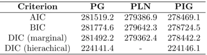
Posterior estimates for the parameters of scientific interest (not presented here) reveal that all regression parameters have statistically significant ef-fects. Interestingly, the posterior means of the PLN and PIG models are closer, especially for the intercept estimate. Model comparison is based on Bayesian versions of AIC and BIC as well as marginal and hierarchical (only for the PG and PIG models) DIC. Results are summarized in Table 1. Marginally, all three criteria give more support to both the PLN and PIG models over the PG model which also explains why the posterior means for the two models are more similar. This result is partially anticipated since the PLN and PIG allow for longer tails and are in theory more appropriate for cases of highly positive-skewed count data (Willmot, 1990). Further-more, all three criteria favour the PIG marginal likelihood more than the PLN marginal likelihood, indicating that the PIG distribution is the most appropriate marginal sampling distribution.
Criterion PG PLN PIG
AIC 281519.2 279386.9 278469.1
BIC 281774.6 279642.3 278724.5
DIC (marginal) 281492.2 279362.4 278442.2
DIC (hierachical) 224141.4 - 224146.1
TABLE 1. The values of AIC, BIC, marginal and hierarchical DIC for the three models.
Based on the hierarchical DIC values, distinguishing a “better” hierarchi-cal model is not as clear as with the marginal models. The value of the PG model is just slightly lower than the corresponding value of the PIG model, therefore a solid conclusion cannot be drawn regarding which model
is more appropriate for predictive purposes. Therefore, predictions are gen-erated from the hierarchical structures of both models. Overall goodness-of-fit predictive tests based on Bayesian p-values indicate satisfactory fit for both models. Nevertheless, particular predictive distributions on aggre-gated levels differ substantially.
5
Conclusions
Statistical OD modeling is advocated as a viable alternative to traditional trip-generation and trip-distribution modeling. To this end, we propose that Poisson mixtures and Bayesian methods provide a suitable framework for modeling large, over-dispersed OD datasets when the focus of interest is not only on parameter estimation but also on short-term prediction. In particular, the performance of the PG, PLN and PIG models was evaluated on a Flemish OD matrix from the 2001 Belgian travel census. The PIG model was found not only to provide the best marginal fit, but that it also has desired distributional properties very much alike the PG model and unlike the rather cumbersome PLN model.
References
Dean, C., Lawless, J. F. and Willmot, G.E. (1989). A mixed Poisson-inverse-Gaussian regression model. The Canadian Journal of Statistics, 17, 171-181.
Lawless, J. F. (1987). Negative binomial and mixed Poisson regression. The Canadian Journal of Statistics , 15, 209-225.
Lee, Y. and Nelder, J.A. (2004). Conditional and marginal models: an-other view. Statistical Science, 19, 219-228.
Nikoloulopoulos, A.K. and Karlis, D. (2008). On modeling count data: a comparison of some well-known discrete distributions. Journal of Sta-tistical Computation and Simulation, 78, 437-457.
Ort´uzar, J. de D. and Willumsen, L.G. (2001). Modeling Transport. Chich-ester: John Wiley and Sons.
Perrakis, K., Karlis, D., Cools, M., Janssens, D., Vanhoof, K. and Wets, G. (2012). A Bayesian approach for modeling origin-destination matri-ces. Transportation Research, Part A, 46, 200-212.
Stopher, P.R. and Greaves, S.P. (2007). Household travel surveys: where are we going? Transportation Research, Part A, 41, 367-381. Willmot, G.E. (1990). Asymptotic tail behaviour of Poisson mixtures with