Cavity quantum electrodynamics and intersubband polaritonics of a two dimensional electron gas

HAL Id: tel-00421386

https://tel.archives-ouvertes.fr/tel-00421386

Submitted on 1 Oct 2009

HAL is a multi-disciplinary open access

archive for the deposit and dissemination of sci-entific research documents, whether they are pub-lished or not. The documents may come from teaching and research institutions in France or abroad, or from public or private research centers.

L’archive ouverte pluridisciplinaire HAL, est destinée au dépôt et à la diffusion de documents scientifiques de niveau recherche, publiés ou non, émanant des établissements d’enseignement et de recherche français ou étrangers, des laboratoires publics ou privés.

Cavity quantum electrodynamics and intersubband

polaritonics of a two dimensional electron gas

Simone de Liberato

To cite this version:

Simone de Liberato. Cavity quantum electrodynamics and intersubband polaritonics of a two di-mensional electron gas. Condensed Matter [cond-mat]. Université Paris-Diderot - Paris VII, 2009. English. �tel-00421386�

UNIVERSIT´

E PARIS DIDEROT (Paris 7)

ECOLE DOCTORALE: ED107

DOCTORAT

Physique

SIMONE DE LIBERATO

CAVITY QUANTUM ELECTRODYNAMICS AND

INTERSUBBAND POLARITONICS OF A TWO

DIMENSIONAL ELECTRON GAS

Th`

ese dirig´

ee par Cristiano Ciuti

Soutenue le 24 juin 2009

JURY

M. David S. CITRIN

Rapporteur

M. Michel DEVORET

Rapporteur

M. Cristiano CIUTI

Directeur

M. Carlo SIRTORI

Pr´esident

M. Iacopo CARUSOTTO Membre

Contents

Acknowledgments 3

Curriculum vitae 5

Publication list 9

Introduction 13

1 Introduction intersubband polaritons physics 19

1.1 Introduction . . . 19

1.2 Useful quantum mechanics concepts . . . 20

1.2.1 Weak and strong coupling . . . 20

1.2.2 Collective coupling . . . 20

1.2.3 Bosonic Approximation . . . 21

1.2.4 The rotating wave approximation . . . 22

1.3 Physical system . . . 23

1.3.1 The doped quantum well . . . 23

1.3.2 The microcavity . . . 25

1.3.3 Intersubband polaritons . . . 27

1.4 Quantum description . . . 29

1.4.1 The full Hamiltonian . . . 29

1.4.2 The RWA fermionic Hamiltonian . . . 31

1.4.3 The bosonic Hamiltonian . . . 32

1.4.4 The RWA bosonic Hamiltonian . . . 34

2 Quantum vacuum radiation phenomena 35 2.1 Introduction . . . 35

2.2 Quantum vacuum radiation as ultra-strong coupling effect . . . 37

2 Contents

2.4 Numerical results . . . 45

2.5 Experiments: ultra-strong coupling . . . 51

2.6 Experiments: ultra-fast modulation . . . 52

2.7 Conclusions and perspectives . . . 54

3 Light emitters in the strong coupling regime 59 3.1 Introduction . . . 59

3.2 Hamiltonian and approximations . . . 60

3.3 Steady-state regime and observable quantities . . . 66

3.4 Numerical procedure and results . . . 69

3.5 Conclusions and perspectives . . . 78

4 Electron tunneling into polariton states 79 4.1 Introduction . . . 79

4.2 General formalism . . . 80

4.3 Spectral function with light-matter interactions . . . 81

4.4 Tunneling coupling, losses and electroluminescence . . . 87

4.5 Conclusions and perspectives . . . 92

5 Intersubband polariton scattering and lasing 93 5.1 Introduction . . . 93

5.2 General formalism . . . 94

5.3 Many-body matrix elements calculation . . . 97

5.4 Scattering rate and lasing threshold . . . 99

5.5 Conclusions and perspectives . . . 103 General conclusions 105 A Second quantized Hamiltonian 107 B Input-output formalism 111 C Factorization scheme 115 D Diagonalization procedure 119 E Matrix elements recursive relation 123

Acknowledgments

There is a quite long list of people who have helped me in different ways during the three years of my Ph.D. and to whom I am greatly indebted.

The first person I have to thank is my advisor Cristiano Ciuti, not only for having always been kind and available, and for having taught me so much, but also for having trusted me enough to grant me complete scientific freedom in these years. He always encouraged me to pursue my ideas, even when completely unrelated to his research and the main body of my thesis. Without his guidance and foresight, a good deal of the work I accomplished during these years would not have been possible.

I also have to thank three colleagues I had the pleasure to work with in mul-tiple occasions during my Ph.D.: Iacopo Carusotto, my unofficial co-advisor; Aji A. Anappara, who had the uneasy task of being the interface between myself and a working experiment; and Luca De Feo, who introduced me to the domain of algorithmic complexity and often accompanied me during my trips through its lands. Then I acknowledge all the other colleagues I had fruitful an pleasant interactions with. Without pretensions of completeness, I want to thank: J´erˆome Faist, Dario Gerace, Rupert Huber, Juan Pablo Paz, Sandu Popescu, Luca Sapienza, Carlo Sirtori, Yanko Todorov and Alessandro Tredicucci.

I would like to thank researchers and administrative staff at Laboratoire Mat´eriaux et Ph´enom`enes Quantiques and Laboratoire Pierre Aigrain (where I performed my undergraduate diploma work) for discussions, assistance and logistical support during my Ph.D. I would like to thank the project ANR INTERPOL and CNRS, who have financed many missions during my Ph.D. years.

Then, in no special order, I want to thank: my father, Luciano De Liberato; my colleagues at Laboratoire Mat´eriaux et Ph´enom`enes Quantiques: Xavier Caillet, Simon Pigeon, Erwan Guillotel, Marco Ravaro and all the others;

4 Acknowledgments Oussama Ammar and all the friends of Hypios; Florian Praden and all my friends at ´Ecole Normale Sup´erieure. It is also a pleasure to thank Alessandro Colombo, Stefano Bertani, Domenico Bianculli and all the other friends I met during my years at the Politecnico di Milano. They made life enjoyable and travel cheap.

A special thanks goes to Alberto Santagostino, because nothing says old

school scientist more than having a Mecenate; to Steve Jobs, because without

him this thesis would not have been 100% Microsoft-free; to Hugh Everett III, for having taken quantum mechanics seriously enough; and to all the people who do not consider shut up and calculate a valid interpretation of quantum mechanics.

Curriculum vitae

Personal data

Name: Simone Surname: De Liberato

Date of birth: 26 September 1981 Nationality: Italian

Education

2006-2009: Ph.D. student at Universit´e Paris Diderot-Paris 7

2005-2006: Master in Quantum Physics at ´Ecole Normale Sup´erieure 2003-2005: Graduation in Physics at ´Ecole Normale Sup´erieure 2000-2003: Student at Politecnico di Milano

6 Curriculum vitae

Conferences, Schools

September 2008: Workshop on Quantum Coherence and Decoherence (Benasque, Spain)

September 2008: ICSCE4 conference (Cambridge, England) July 2008: ICPS08 conference (Rio De Janeiro, Brazil) June 2008: Fermi Summer School (Varenna, Italy)

December 2007: 25th Winter School in Theoretical Physics at the IAS (Jerusalem, Israel)

July 2007: EP2SD 17 + 13 MSS conference (Genova, Italy)

June 2007: Vienna Symposium on the Foundations of Modern Physics (Wien, Austria)

September 2006: XXIV Convegno di Fisica Teorica e Struttura della Materia (Levico Terme, Italy)

June 2006: Poise Summer School (Cortona, Italy)

July 2004: Diffiety Summer School (Santo Stefano del Sole, Italy)

Internships

July-September 2008: Visiting scholar at the University of Buenos Aires, in the group of Prof. Juan Pablo Paz

January-July 2006: Internship at Laboratoire Pierre Aigrain (ENS Paris) under the direction of Prof. C. Ciuti

February-August 2005: Internship at Clarendon Laboratory (Oxford, England) under the direction of Prof. C. J. Foot

June-August 2004: Internship at University Tor Vergata (Rome, Italy) under the direction of Prof. M. Cirillo

7

Teaching Experience

2006-2009: Teaching assistant at Universit´e Pierre et Marie Curie, for the class LP104, Introduction to physics

Spoken Languages

Publication list

Publications treated in this manuscript

7. Signatures of the ultra-strong light-matter coupling regime

A. A. Anappara, S. De Liberato, A. Tredicucci, C. Ciuti, G. Biasiol, L. Sorba and F. Beltram

Physical Review B 79, 201303(R) (2009)

6. Stimulated scattering and lasing of intersubband cavity polaritons S. De Liberato and C. Ciuti

Physical Review Letters 102, 136403 (2009)

5. Sub-cycle switch-on of ultrastrong light-matter interaction

G. Guenter, A. A. Anappara, J. Hees, G. Biasiol, L. Sorba, S. De Liber-ato, C. Ciuti, A. Tredicucci, A. Leitenstorfer, and R. Huber

Nature 458, 178 (2009)

4. Quantum theory of electron tunneling into intersubband cavity polariton

states

S. De Liberato and C. Ciuti

Physical Review B 79, 075317 (2009)

3. Quantum model of microcavity intersubband electroluminescent devices S. De Liberato and C. Ciuti

10 Publication list 2. Cavity polaritons from excited-subband transitions

A. Anappara, A. Tredicucci, F. Beltram, G. Biasiol, L. Sorba, S. De Lib-erato and C. Ciuti

Applied Physics Letters 91, 231118 (2007)

1. Quantum vacuum radiation spectra from a semiconductor microcavity

with a time-modulated vacuum Rabi frequency

S. De Liberato, C. Ciuti and I. Carusotto Physical Review Letters 98, 103602 (2007)

Other publications

4. Fermionized photons in an array of driven dissipative nonlinear cavities I. Carusotto, D. Gerace, H. Tureci, S. De Liberato, C. Ciuti and A. Imamo˘glu

Physical Review Letters 103, 033601 (2009)

In this paper we theoretically investigated the optical response of a one-dimensional array of strongly nonlinear optical microcavities. We discov-ered than when the optical nonlinearity is the dominant energy scale, the non-equilibrium steady state of the system is reminiscent of a strongly correlated Tonks-Girardeau gas of impenetrable bosons.

3. Optical properties of atomic Mott insulators: from slow light to the

dy-namical Casimir effects

I. Carusotto, M. Antezza, F. Bariani, S. De Liberato and C. Ciuti Physical Review A 77, 063621 (2008)

In this paper we theoretically studied the optical properties of a gas of ul-tracold, coherently dressed three-level atoms in a Mott insulator phase of an optical lattice. In the weak dressing regime, the system shows unique ultra-slow light propagation properties without absorption. In the pres-ence of a fast time modulation of the dressing amplitude, we predicted a significant emission of photon pairs due to the dynamical Casimir effect.

11 2. Observing the evolution of a quantum system that does not evolve

S. De Liberato

Physical Review A 76, 042107 (2007)

In this paper I studied the problem of gathering information on the time evolution of a quantum system whose evolution is impeded by the quantum Zeno effect. I found it is in principle possible to obtain some information on the time evolution and, depending on the specific system, even to measure its average decay rate, even if the system does not un-dergo any evolution at all. This paper has been reviewed by L. Vaidman in a News & Views on Nature [1].

1. Tunnelling dynamics of Bose-Einstein condensate in a four wells loop

shaped system

S. De Liberato and C. J. Foot

Physical Review A 73, 035602 (2006)

In this brief report, whose research was performed during an undergrad-uate internship in the group of C. J. Foot, I studied some properties of Bose-Einstein condensates in loop geometries, with particular attention to the creation and detection of currents around the loop.

Introduction

The history of cavity quantum electrodynamics, the study of light-matter in-teraction in quantum confined geometries, started when Purcell [2] noted that the spontaneous emission rate of an excited atom can be changed by adjusting the boundary conditions of the electromagnetic field with properly engineered cavities. Since then, experiments showing modifications of spontaneous emis-sion rates were realized with ever-growing atom-cavity couplings and cavity quality factors [3, 4, 5, 6, 7]. This lead eventually to systems in which the pho-ton lifetime inside the cavity was substantially bigger than the spontaneous emission rate, that is systems in which a single photon undergoes multiple ab-sorption and reemission cycles before escaping the cavity [8, 9, 10]. The first experiments that reached this regime, named strong coupling regime, were performed with Rydberg atoms in superconducting cavities. Strong coupling regime was then achieved in solid-state systems, using quantum well excitons in microcavities [11] and, more recently, Cooper pair boxes in superconducting circuits [12] (in this case the name circuit quantum electrodynamics is often employed).

But what does strong coupling exactly means? Textbooks normally define two coupled systems to be strongly coupled if it is possible to experimentally resolve the energy shift due to the coupling, that is the coupling constant (quantified by the vacuum Rabi frequency ΩR) needs to be bigger than the

linewidth of the resonances. If two systems are strongly coupled, the com-posite system eigenstates can not be described as a tensorial product of the eigenstates of the two bare ones. That is the interaction is so strong that entan-gles the systems and the only meaningful information becomes the eigenstate of the coupled system. In the case of two level systems (e. g. the Rydberg atoms in microwave cavities), people usually calls these eigenstates of dressed

states, in the case of bosonic ones (e. g. excitons in planar microcavities), the

14 Introduction In the last ten years, exciton polaritonics has become a remarkably rich field in condensed matter physics, fertile both for fundamental and applied research [13, 14, 15, 16, 17, 18, 19]. In such systems, thanks to the small polaritonic mass (inherited from their photonic part), it is possible to reach the quantum degenerate regime at temperatures orders of magnitude bigger than in atomic systems. Exciton polariton Bose-Einstein condensation was recently achieved at a temperature of few kelvin [20], compared to hundreds of nanokelvin needed for atomic cloud Bose-Einstein condensates. New kinds of electroluminescent [21] and lasing [22, 23] devices have been realized with such quasi-particles, often with unprecedented performances.

In 2003 there was a new entry in the list of solid-state strongly coupled systems with the first experimental observation of the strong coupling be-tween a microcavity photon mode and the intersubband transition of a doped quantum well [24]. Intersubband transitions are named in opposition to the usual interband transitions, occurring between valence and conduction band in semiconductors. They are instead transitions between the subbands in which the conduction band is split due to the quantum well confinement. While this kind of polaritons, quickly dubbed intersubband polaritons, are in vari-ous respect profoundly different from exciton polaritons, both for the energy range (mid-infrared to Terahertz) and for the nature of the electronic transi-tion (intersubband transitransi-tions, contrary to excitons, are not bound states), the main interest of these new polaritons stays in the strength of the light-matter interaction [25].

We just mentioned that the light-matter coupling in these systems, as for excitons or atoms, can be strong. Is it possible to go further? The definition of strong coupling in term of energy shifts and linewidths is clearly relevant in spectroscopic experiments: two systems are strongly coupled if we can resolve the effect of the interaction, which produces an energy anticrossing between light and matter resonances. Anyway it does not permit to make any assess-ment on the real strength of the interaction. Being in the usual strong coupling regime means to have an energy shift due to coupling bigger than the linewidth of the resonance, that can be achieved even with extremely small couplings, if the losses are small enough. In order to assess the real strength of the in-teraction, the right figure of merit is the ratio between the interaction energy and the bare system excitation energy ~ω12 (transition energy). The ratio _ωΩ₁₂R

gives a direct assessment of the relative strength of the interaction, not of our ability to spectroscopically observe it.

15 In atomic systems ΩR

ω12 is typically less then 10

−6 _{in the case of a single}

atom. That is the atomic transition resonance shifts of less than one part per million from its unperturbed position. We can still see the shift simply because superconducting cavity can have an astounding quality factor, of the order of 109_{, that permits us to resolve even such tiny shifts. Is it possible}

to do better? Not in dilute atomic systems [26], where the smallness of this ratio directly depends upon the small value of the fine structure constant α ≃ 1

137. In condensed matter cavity quantum electrodynamics it is possible

to beat this limit, exploiting collective, coherent excitations. If a large number of electrons gets collectively excited, the ensuing excitation has a collective dipole, whose intensity scales as the square root of the electron number, in a phenomenon reminiscent of the Dicke superradiance [27]. In excitons for example, where a large number of valence electron states participates to the excitation, experiments have reached values up to 10−2 _{for the ratio} ΩR

ω12 [28,

29, 30, 31].

In intersubband excitations, the values obtained until now are bigger than 10−1_{, and there is still a large marge of improvement [32]. That is, the}

cou-pling is intrinsically strong, enough to significatively change the spectrum of the system and the nature of the quantum ground state. Other systems in which such large couplings could be achieved are Cooper pair boxes coupled to superconducting line resonators, where theoretical values up to 20 have been predicted [26]. This regime of intrinsic strong coupling was named ultra-strong

coupling. Such ultra-strong coupling is interesting for various reasons. In

par-ticular the ground state turns out to be a squeezed vacuum, containing pairs of virtual photons [25, 33].

While such virtual excitations are normally unobservable, they can become real if the system is modulated in a non-adiabatic way [34]. This effect, the emission of photons out of the ground state when the system is perturbed, is a manifestation of the dynamical Casimir effect [35], an elusive and never observed quantum electrodynamics effect reminiscent of the Unruh effect [36] (colloquially speaking the dynamical Casimir effect predicts that a mirror, shaken in the vacuum, emits photon pairs, the Unruh effect predicts that a thermometer, shaken in the vacuum, measures a non-zero temperature). Intersubband polaritonic systems, together with Cooper pair boxes, seems to be very promising systems for observing this kind of effects.

On a more applied ground, it is important to point out that the light matter coupling could affect electric transport and electroluminescence, opening new

16 Introduction opportunities that could be exploited to create high-efficiency light sources in the mid-infrared and Terahertz regions.

The manuscript consists of five chapters. Chapter 1 serves as a general in-troduction and reference, the other four follow quite chronologically my Ph.D. work of the last three years. Chapter 2 presents a comprehensive quantum Langevin theory predicting the quantum vacuum radiation induced by the non-adiabatic modulation of the vacuum Rabi frequency in microcavity em-bedded quantum wells. The theory accounts both for ultra-strong light-matter excitations and losses due to the coupling with radiative and non-radiative baths. Chapter 2 also reports of two experimental milestones [32, 37] toward the observation of such effect.

Chapters 3 and 4 present a general theory to describe the influence of inter-subband polaritons on electron transport and electroluminescence. Chapter 3 presents a numerical method [38] capable to model electrical transport through a microcavity embedded quantum well, taking into account the strong cou-pling of electrons with the microcavity photons. Not only it gives a theoretical explanation to various features observed in electroluminescence experiments [39], but it also shows that, by increasing the light matter coupling in such devices, it may be possible to drastically increase their quantum efficiency, in a strong coupling extension of the Purcell effect [2]. Chapter 4 shows how the coupling with the quantum vacuum fluctuations of the microcavity electromag-netic field can qualitatively change the spectral function of the electrons inside the structure. The spectral function is characterized by a Fano resonance, due to the coupling of the electrons with the continuum of intersubband polari-tons. The theory suggests that these features may be exploited to improve the quantum efficiency by selectively excite superradiant states through resonant electron injection. Finally Chapter 5 shows how it is possible to exploit the peculiar properties of intersubband polaritons in order to obtain a new kind of inversionless laser [40]. A theory of polariton stimulated scattering due to interaction with optical phonons is developed, that fully takes into account saturation effects that make the behavior of intersubband polaritons to depart from the one of pure bosons. With realistic parameters, this theory predicts lasing with a threshold almost two orders of magnitude lower than existing intersubband lasers.

Sometimes the algebra behind the presented results may be heavy. In order to improve readability I reduced to the minimum the quantity of equations in the main body of the text, moving all the technical calculations in the

Appen-17 dices. Each Chapter has thus its own Appendix, in which the reader interested in technical details will find all the calculations that were not included neither in the corresponding Chapter, nor in Letter format publications.

Chapter 1

Introduction intersubband

polaritons physics

1.1

Introduction

A number of the following chapters are dedicated to solve various problems linked with the physics of quantum coherent phenomena in microcavity em-bedded quantum wells. In order to keep the chapters independent, avoiding both boring repetitions and too many inter-chapter references, I decided to collect in this first chapter all the notions necessary for the comprehension of this thesis.

I will start giving an overview of different quantum mechanical concepts. I think that almost all of them are considered as common background for working scientists in condensed matter physics, anyway I prefer to review them, especially because the aspects I am interested in are often not the ones stressed in textbooks. Then I will give a brief review of the physics of quantum wells, microcavities and of their interactions. In the last part I will introduce the main theoretical tools I will need, that is the many body Hamiltonian for the system, in its full form as well as in different simplified forms that will be useful for treating different problems.

20 Chapter 1. Introduction intersubband polaritons physics

1.2

Useful quantum mechanics concepts

1.2.1

Weak and strong coupling

In basic quantum mechanics, when describing the evolution of a system, it is customary to make a strong distinction between the case in which the initial state of such system is coupled only to another discrete state or instead to a

continuum of final states. In the first case the dynamics exhibits oscillations,

called Rabi oscillations, while in the second case the dynamics is irreversible and usually described by means of the Fermi golden rule.

The apparent dichotomy between these two cases is given by the fact that, due to the coherent nature of quantum mechanics, the initial state couples at the same time to all the possible final states. If the different final states have different energies anyway they will oscillate at different frequencies and thus, even if for long times we expect to still observe Rabi oscillations (or more precisely quantum revival of Rabi oscillations [41, 42, 43]), for short times the phase of the system is randomized on a timescale of the order of the inverse of the continuum frequency width. If this randomization is faster than the Rabi oscillation period, the coherence is lost before even one single oscillation can take place.

It is easy to understand that the real dichotomy is not between a discrete level and a continuum but between a narrow and a broad continuum, where the width of the continuum has to be compared with the frequency of the Rabi oscillations. For this reason the two regimes are called strong and weak coupling respectively, where weak and strong refer to the strength of the cou-pling, that is proportional to the frequency of the Rabi oscillations. Clearly this definition is equivalent to the more common definition of weak and strong coupling between two coupled systems based on the possibility to resolve the energy anticrossing of the eigenmodes induced, at resonance, by the coupling.

1.2.2

Collective coupling

The phenomenon of superradiance, usually known as Dicke superradiance [27, 44, 45, 46], is basically the drastic enhancement in the spontaneous emission rate of a collection of coherently excited two level systems. This concept has a broad interest, both for fundamental and applied reasons, and it is crucial to almost all the results of this thesis. For this reason I will give here an extremely short introduction on superradiance from a point of view that, while

1.2. Useful quantum mechanics concepts 21 quite different from the standard textbook definition, is specifically useful for the present work. Superradiance is a consequence of a very basic property of quantum mechanics. If a quantum state |ψi is identically coupled with N degenerate states _|φji then, applying an unitary transformation on the

degenerate subspace _{|φji}, we can redefine the states in order to have the

initial state coupled to a single final state, with a coupling constant √N times bigger than the bare one. The proof of this statement is simple linear algebra. The system Hamiltonian, calling ~ω the energy of the initial state and choosing as zero the energy of the degenerate subspace is

H = ~ω_{|ψihψ| + ~Ω}

N

X

j=1

|ψihφj| + |φjihψ|. (1.1)

Applying to the to the degenerate subspace a linear transformation that maps {|φji} to {| ¯φji} such that | ¯φ1i = √1_N Pj|φji and the other vectors are

deter-mined by orthonormality, we obtain ¯

H = ~ω|ψihψ| +√N~Ω(|ψih ¯φ1| + | ¯φ1ihψ|). (1.2)

We see that in the new Hamiltonian there is only one state coupled to the initial one with an enhanced coefficient, while the other N _{− 1 are uncoupled} and have disappeared from the Hamiltonian.

1.2.3

Bosonic Approximation

The main manifestation of electrons fermionic nature is the existence of Pauli blocking, only one electron can occupy each quantum state at a given time. For an electronic transition between an initial and a final state to be possible we need to have both the initial state full and the final state empty. This means that a collection of N two level systems can only be excited N times before it saturates. For example in a semiconductor, if a significant fraction of valence electrons are pumped into the conduction band, further electrons have a reduced phase space to jump and the light-matter interaction decreases. On the contrary a single bosonic oscillator can absorb an unlimited number of excitations. Given the extreme ease we have in treating bosonic fields, it is tempting, at least as long as we are far from saturation, that is if the number of excitations n is much smaller than N, to approximate the collective excitation of many two level systems with a single bosonic mode.

22 Chapter 1. Introduction intersubband polaritons physics There is indeed a deeper link between a bosonic field and an ensemble of fermionic transitions. To consider the latter as a boson is substantially the same approximation we make when we say that an atom with an even number of fermions acts as a boson. Formally we can describe a two level system by means of two second-quantized fermionic fields, c1 and c2. For example a

transition between the first and the second level will be given by the operator b† _{= c}†

2c1, that is an electron is annihilated in the first level and is created in

the second one. The property of fermionic fields (c2

1 = c22 = 0) assures that

such transition is possible only if the first level is full and the second one empty. If we consider a collection of N of such two level systems, indexed by an index j, it is easy to verify that, if _{|ψi is a state such that n systems are excited,} then on average _hψ|[bj, b†_j′]|ψi = δj,j′+ O(n

N). That is, the operators bj, being

composed of an even number of fermions have, at low excitation densities, the commutation relations of bosonic fields.

1.2.4

The rotating wave approximation

The rotating wave approximation (RWA) is an approximation scheme consist-ing of neglectconsist-ing highly nonresonant (that is quickly oscillatconsist-ing) terms in the Hamiltonian. The RWA is used over almost all the domains of physics, from astronomy to quantum mechanics and permits the exact solution of various otherwise intractable problems.

The breaking of this approximation, or more precisely the physics that emerges if this approximation is not valid, will be an important part of Chapter 2. I will thus take some time here to review the basics of the RWA by analyzing its application to a really simple quantum system.

Let us consider the Hamiltonian of two coupled resonant harmonic os-cillators, whose second quantization annihilation operators are a and b, the frequency is ω and the coupling strength Ω. The Hamiltonian is thus

H = ~ω(a†a + b†b) + ~Ω(a + a†)(b + b†). (1.3) Applying the RWA on the system described by Eq. 1.3 means neglecting the terms ab and a†_b†_{. These terms connect states with a bare energy difference}

of 2ω and thus their contribution in second order perturbation theory (i.e. to the energy of the ground state) is of the order of

∆2 =

Ω2

1.3. Physical system 23 If ω _{≫ Ω the effect of antiresonant terms is thus suppressed. This is the case} in almost all non-driven physical systems. Only in the last few years a number of propositions [47, 48, 26, 25, 33, 34, 32] have been put forward of systems not fulfilling the RWA.

1.3

Physical system

1.3.1

The doped quantum well

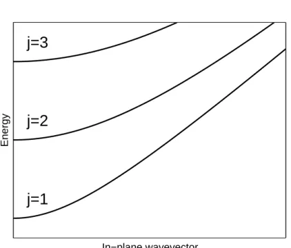
A quantum well is a planar heterostructure that quantum confines electrons along the growth axis. This tight confinement strongly influences the density of states of the electrons, that effectively behave as a two dimensional electron gas (2DEG). The confinement in fact splits the electronic Bloch bands into discrete subbands, in Fig. 1.1 it is shown the typical band structure and in-plane dispersion of a quantum well. The electrons are free to move in the in-plane normal to the growth direction with an effective mass given by the subband dispersion ~ωj,n(k), where j = v, c is the band index, k is the component

of the wavevector in the plane normal to the growth direction and n is an integer giving the subband index. An electronic state in the quantum well will thus be indexed by the two components of the in-plane wavevector kx

and ky (we will consistently suppose that the growth direction is along the z

axis), the band index, the subband index and the spin. The Fermi level of a quantum well, that in an intrinsic semiconductor would be in the gap between the highest energy valence subband and the lowest energy conduction subband, can be easily shifted by doping. This permits to select which of the multiple interband and intersubband transitions is optically active. In the rest of the thesis we will be interested in the coupling of intersubband transitions with light, thus we will consider quantum wells whose Fermi level is between the first and the second conduction subband, even if experimentally other cases are possible [49]. The main interest of considering such transitions is that, due to the parallelness of the conduction subbands and the smallness of the photon wavevector, the 2DEG behave approximately as a collection of two level systems with the same transition frequency. In fact being the photonic wavevector much smaller than the electronic one, photonic induced transitions are almost vertical on the scale of the electronic dispersions of Fig. 1.1. As we have seen in Section 1.2.2 a collection of two level systems coupled to the light can be seen as a single system with a coupling √N times bigger. This is

24 Chapter 1. Introduction intersubband polaritons physics e h Conduction band Valence band E gap ¯hω_{1 2}

Position along the z axis

Confinement potential E gap ¯hω_{1 2} In−plane wavevector Energy

Figure 1.1: Top panel: schema representing the band structure of a semicon-ductor quantum well. The electronic confinement and the presence of subbands are well visible. Bottom panel: the corresponding band dispersion, as a func-tion of the wavevector in the plane normal to the growth direcfunc-tion.

1.3. Physical system 25 exactly what happens in the case of intersubband transitions. Only one linear superposition of electronic transitions, called bright intersubband excitation, is coupled to the light field, but with a dipole√N times bigger than the bare one, where N is the number of electrons in the 2DEG. Such dipole is oriented along the z axis, giving a polarization selection rule for intersubband excitations, only Transverse Magnetic (TM) polarized light couple to the quantum well, while Transverse Electric (TE) polarized photons are completely decoupled.

1.3.2

The microcavity

In order to increase the coupling between light and matter, it is favorable to increase the spatial overlap between the photonic modes and the matter excitations. This is at the heart of the so called Purcell effect [2]. In order to increase this overlap it is necessary to confine the photonic mode inside a cavity. A number of different cavity technologies have been devised, spanning different geometries and frequency ranges: from superconducting microwaves [50] to one dimensional transmission lines [51]. In condensed matter systems the interest in increasing the light-matter coupling is not only linked with the possibility to observe interesting new physics [34] but also to the engineering of efficient light emitters [52, 38]. This interest has led to the conception of different kinds of microcavities with planar geometries that can be directly embedded in semiconductor heterostructures. The confinement of the photonic mode can be obtained using dielectric Bragg mirrors, metallic mirrors or even exploiting total internal reflection.

The effect of a planar microcavity is to quantize the photon wavevector along the growth direction. The photonic dispersion is thus given by

ωcav, j(q) = c √_ǫ r q q2_{+ q}2 z,j, (1.5)

where qz,j is the j-th value of the quantized qz vector. A typical dispersion is

shown in Fig. 1.2.

It is worthwhile to notice the parabolic dispersion around q = 0, photons gets an effective mass due to the confinement. In the following we will work in a regime in which the intersubband gap energy ~ω12 is resonant with a mode

on the first cavity branch. We will thus limit ourselves to consider the first photonic branch, being the others well out of resonance.

26 Chapter 1. Introduction intersubband polaritons physics

j=1

j=2

j=3

Figure 1.2: Energy dispersion of a planar microcavity as a function of the wavevector in the plane normal to the growth direction. The index j indexes different photonic branches corresponding to different values of the quantized wavevector along the growth direction.

1.3. Physical system 27

1.3.3

Intersubband polaritons

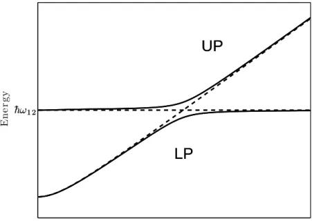
When the microcavity is resonant with the intersubband transition energy ~_{ω12, due to the strength of the coupling between an intersubband excitation} and a microcavity photon, the system can be in the strong coupling regime. In Fig. 1.3 it is shown a typical dispersion of the system resonances as a function of the in-plane wavevector. Dashed lines are the bare resonances of the inter-subband transition and of the microcavity photons, while solid lines are the dispersions of normal modes of the coupled system. At resonance, the anti-crossing between the dispersions of the two normal modes is clearly visible. In this regime the new eigenmodes of the system are called intersubband polari-tons. The experimental observation of their resonances has been reported for the first time in [24]. Their data with the anticrossing of reflectance resonances can be found in Fig. 1.4. Another, more recent observation of polariton

UP

LP

UP

LP

Figure 1.3: Energy dispersions of excitations in a microcavity embedded quan-tum well as a function of the wavevector in the plane normal to the growth direction. Dashed lines represent the dispersion of the intersubband excitation (dispersionless) and of the bare microcavity photon mode. Solid lines represent the upper (UP) and lower (LP) polariton branches.

28 Chapter 1. Introduction intersubband polaritons physics

Figure 1.4: Experimental data from Ref. [24]. The reflectance spectra for various angles show clearly the level anticrossing. This is the first experimental observation of intersubband polariton dispersions.

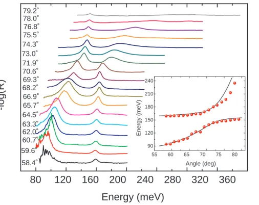
1.4. Quantum description 29 nances in a quantum cascade structure is shown in Fig. 1.5. In Fig. 1.6 there is a sketch of the mesa etched sample and of the corresponding band diagram (Both images are from Refs. [53] and [39]).

80

120

160

200

240

280

320

360

-log(R)

Energy (meV)

Figure 1.5: Reflectivity spectra as a function of the incident angle. In the inset the position of the peaks (full dots) is compared with the theoretical results of transfer matrix calculations (line). Image taken from Ref. [39].

1.4

Quantum description

1.4.1

The full Hamiltonian

In order to elaborate a theory of a microcavity embedded two dimensional electron gas, we will need to derive the second quantization Hamiltonian for such system. The quantum fields we need to describe are the microcavity photon field and the electron fields in the first and second subbands. We thus introduce the electron creation fermionic operators in the first and second subband (c†_1,σ,k and c†_2,σ,k), and the bosonic creation operator a†_ζ,q, where σ is the electron spin, ζ the photon polarization, while k and q are the in-plane

30 Chapter 1. Introduction intersubband polaritons physics

§

T

undoped GaAs substrate Al0.95Ga0.05As n-doped GaAs

QC

(a)

(b)

thickness (Angstrom)

E

n

e

rg

y

(

e

V

)

Figure 1.6: Top panel: schema of the mesa etched sample of Ref. [53]. Bottom panel: band diagram of the quantum cascade structure. Images taken from Ref. [53].

1.4. Quantum description 31 wavevectors. Systematically in this thesis, I will use the letters k and q for the electronic and photonic wavevector respectively. This distinction will often be useful due to the smallness of photons wavevectors compared to electronic ones.

The Hamiltonian, whose exact derivation is detailed in Appendix A, is H = X k ~_ωc,1(k)c† 1,kc1,k+ ~ωc,2(k)c†2,kc2,k (1.6) + X q ~_ωcav(q)a† qaq+ ~D(q)(a_1,−q+ a†1,q)(a1,q+ a†_1,−q) + X k,q ~_{χ(q)(aq+ a}† −q)c†2,k+qc1,k+ ~χ(q)(a−q+ a†q)c†1,kc2,k+q.

The energy dispersions of the two quantum well conduction subbands, shown in Fig. 1.1 as a function of the in-plane wavevector k, are ~ωc,1(k) =

~2_k2

2m⋆ and

~_{ωc,2(k) = ~ω12+} ~2k2

2m⋆, being k the electron in-plane wavevector and m⋆ the

effective mass of the conduction subbands (non-parabolicity is here neglected, see Ref. [54]).

As explained in detail in A, we neglect the electron spin, because all the interactions are spin-conserving. Due to selection rules of intersubband tran-sitions, we omit the photon polarization, which is assumed to be TM. For simplicity, we consider only a photonic branch, which is quasi-resonant with the intersubband transition, while other cavity photon modes are supposed to be off-resonance and can be therefore neglected. Due to the light-matter interaction terms, which are product of three operators, the Hamiltonian in Eq. 1.6 is of formidable complexity, in order to make it tractable, studying different problems we will make various kinds of (controlled) approximations.

1.4.2

The RWA fermionic Hamiltonian

When the light-matter coupling is not too big compared to the intersubband transition frequency, we can safely apply the RWA to the Hamiltonian in Eq. 1.6. This is equivalent to neglect terms in a2

q that annihilate pairs of photons

and terms of the form a†_−qc†_2,k+qc1,k that describe an electron jumping from

32 Chapter 1. Introduction intersubband polaritons physics is thus HRWA = X k ~_ωc,1(k)c† 1,kc1,k+ ~ωc,2(k)c†2,kc2,k+ X q ~_{[ωcav(q) + 2D(q)]a}†_qaq + X k,q ~_χ(q)aqc† 2,k+qc1,k+ ~χ(q)a†qc†1,kc2,k+q. (1.7)

This Hamiltonian, even if it cannot describe regimes of extremely strong cou-plings, retains all the nonlinearities due to Pauli blocking and can describe both low excited or extremely high excitation regimes. More important for us it retains, contrary to the bosonized Hamiltonian we will see in the next section, the description at the level of the single electron, that is necessary when trying to describe electronic transport.

1.4.3

The bosonic Hamiltonian

The large dopant densities usually used in intersubband polariton experiments (of the order of 1012 _cm−2_{) and thus the large number of electrons involved,}

make the numerical study of Hamiltonian in Eq. 1.6 a formidable task. A way to proceed is to notice that even if a large number of electrons participate in the light-matter interaction, only few degrees of freedom are effectively excited. If we do not bother to lose the possibility to describe the system at the level of single electron, we can thus exploit the techniques developed in Section 1.2.3 and bosonize the [55, 56] Hamiltonian in Eq. 1.6. We thus define N bosonic intersubband transition operators as

bj_q = √1 N X k β_kjc†_2,k+qc1,k. (1.8) where β1

k= 1∀k and the other N − 1 β j

k are determined with an

orthonormal-ization procedure.

If we are working in the diluted regime, that is if the number of excitations we wish to treat is much smaller than the number of electrons, it is easy to verify that these operators behave like bosons. If we take the state |ni to be a state with all the electrons in the first subband, except for n that are in the second one, we have

hn|[bjq, b j′_† q′ ]|ni = δ(q − q′)δj,j′+ O( n N) (1.9) hn|[bjq, b j′ q′]|ni = 0.

1.4. Quantum description 33 We have thus not only greatly reduced the number of dynamical degrees of freedom, but we have also transformed a cubic Hamiltonian in a quadratic, bosonic one. Again this approximation, as can be seen from Eq. 1.9, is valid only in the diluite regime, where the excitations do not see each other and fermionic saturation effects do not impair intersubband excitations bosonicity. We will see in Chapter 5 how to deal with bosonization at higher excitation densities.

The energy of such intersubband transition excitations can be found by calculating the average value of Hamiltonian over the state bj †

q |F i, where |F i =

Q

k<kF c

†

1,k|0i is the system ground state with all the electrons in the first

subband, that we use also as zero of energy and _{|0i is the vacuum state for the} electron and photon modes (c1,k|0i = c2,k|0i = aq|0i = 0). We obtain

hF |bj qHbj †q |F i = ~ N X k [ω2(k + q)− ω1(k)]. (1.10)

Given the smallness of the photonic wavevector q compared to the electronic one k, we can safely consider ω2(k + q)− ω1(k) ≃ ω12 and thus obtain the

bosonic effective Hamiltonian: HBos = X q ~_{[ωcav(q) + 2D(q)]a}†_qaq+X j ~_ω12bj †_{q b}j_{q+ ~ΩR(q)(a}†_qb1_{q+ aqb}1 †_{q )} + ~ΩR(q)(aqb1_−q+ a†qb−q1 †) + ~D(q)(aqa−q+ a†qa†−q). (1.11) where ΩR(q) = √

Nχ(q) is the effective vacuum Rabi frequency. It is clear the affinity of transformation in Eq. 1.8 and the superradiant states defined in section 1.2.2. Of the N possible intersubband transitions for a given in-plane wavevector q, only one linear superposition is coupled with the microcavity photon field, with a coupling constant √N times bigger than the coupling constant of a single electron and the other N − 1 excitations are not coupled at all. We will call the former a bright intersubband excitation and the others

dark intersubband excitations. Being the dark excitations uncoupled, when

interested only in optically active excitations, we will drop them out of the Hamiltonian and for simplicity we will call bq the bright excitation

HBos =

X

q

~_{[ωcav(q) + 2D(q)]a}†_{qaq+ ~ω12b}†_{qbq+ ~ΩR(q)(a}†_{qbq+ aqb}†_q) + ~ΩR(q)(aqb−q+ a†qb†−q) + ~D(q)(aqa−q+ a†qa†−q). (1.12)

34 Chapter 1. Introduction intersubband polaritons physics

1.4.4

The RWA bosonic Hamiltonian

If together will all the conditions to be able to use Hamiltonian in Eq. 1.12, we have also a ratio ΩR

ω12 small enough for being in the RWA regime, we can

apply the RWA to Hamiltonian in Eq. 1.12. This means to neglect terms that creates or annihilates pairs of excitations. The resulting Hamiltonian is thus

H_BosRWA = X

q

~_{[ωcav(q) + 2D(q)]a}†_{qaq+ ~ω12b}†_{qbq+ ~ΩR(q)(a}†_{qbq+ aqb}†_q). (1.13)

Chapter 2

Quantum vacuum radiation

phenomena

2.1

Introduction

One of the better known predictions of quantum theory is that the empty space is filled with the vacuum energy of the zero-point fluctuations of the quantum electromagnetic field. This zero-point energy is not measurable in empty space, but if we introduce boundary conditions that make its density inhomogeneous, we can in principle measure the resulting force. In the static case such inhomogeneous zero-point energy gives rise to the so called Casimir force , an usually attractive (but sometime repulsive [57]) force between two conducting bodies in the vacuum. The Casimir effect has been measured with great precision in a number of different experimental setups [58, 59, 60].

If the boundary conditions are time-varying a new class of phenomena arises, in which the zero-point fluctuations of the electromagnetic field are transformed into real photons. This effect is often referred to as dynami-cal Casimir effect [35]. Theoretidynami-cal predictions show that a conducting plate, nonuniformly accelerated in the vacuum, can emit (see Fig. 2.1 for a pictorical visualization of the phenomenon). This emission is due to vacuum fluctuations that exert on the plate a sort of viscous friction that slows it down. Mechani-cal energy is then dissipated in the environment as propagating photon pairs. The radiation generated by a time-modulation of the quantum vacuum is a very general and fascinating phenomenon, bearing various analogies with the Unruh-Hawking radiation [36, 61] in the curved space-time around a black hole. However, contrary to the static case, dynamic effects due to the modulation of

36 Chapter 2. Quantum vacuum radiation phenomena

Figure 2.1: An artist view of the dynamical Casimir effect, by G. Ruoso. the quantum vacuum have not yet been observed due to the extremely small number of photons emitted for realistic mechanical accelerations. Even using as accelerating plates the vibrating mirrors of high-finesse Fabry-P´erot res-onators [62, 63], in order to enhance the intensity of the quantum vacuum radiation, the predicted emitted radiation is very challenging to be measured. A big step toward an experimental verification of the dynamical Casimir effect has been the idea to consider, instead of a cavity with moving mirrors, a fixed cavity with a time-varying refractive index [64, 65]. From the point of view of a cavity photon, what is important is the effective optical length of the cavity, given by the bare cavity length times the refractive index of the cavity dielec-tric spacer. Modulating the refractive index at high frequency anyway is much simpler than modulating the cavity length, as we have to deal only with the in-ertia of the dielectric properties, not with the mechanical motion of the whole solid. Still, the very weak intensity of the emitted radiation has so far hindered its experimental observation. Working on this line, we discovered that in the case of microcavity embedded quantum wells, the unprecedented strength of the light-matter coupling permits to have a Casimir radiation strong enough to be measured with present day technologies. We were able to estimate both the intensity and the spectral signature of emitted radiation [34]. An exper-imental realization of our proposal has been built up and has recently given some results, which are very promising towards the observation of quantum vacuum radiation [37]. Other groups are also working on the idea of exploiting ultra-strong light-matter coupled systems for dynamical Casimir experiment.

2.2. Quantum vacuum radiation as ultra-strong coupling effect 37 Especially interesting are experiments exploiting superconducting transmission lines [66] and qubits [47, 26].

2.2

Quantum vacuum radiation as ultra-strong

coupling effect

Quantum vacuum radiation, that is the emission of light from a time-dependent vacuum, is often theoretically described (and calculated) as the consequence of field quantization with time-dependent boundaries [65]. In our case we will adopt a different point of view that, while allowing us to calculate all the system observables, will give a much more intuitive understanding of the process and underline the importance of working in a regime of ultra-strong light-matter interaction.

Let us consider a microcavity embedding multiple quantum wells, as de-scribed in Section 1.3. The photon emission is due to the light-matter coupling, so that only light-coupled matter excitations play a role. In order to describe the system we will thus use the bosonic Hamiltonian of Section 1.4.3

Hbos =

X

q

~_{[ωcav(q) + 2D(q)]a}†_{qaq+ ~ω12b}†_{qbq+ ~ΩR(q)(a}†_{qbq+ aqb}†_q) + ~ΩR(q)(aqb_−q+ a†qb†−q) + ~D(q)(aqa_−q+ a†qa†−q). (2.1)

As all the terms in the Hamiltonian are bilinear in the field operators, it can be exactly diagonalized through a Hopfield-Bogoliubov transformation [55]. Introducing the Lower Polariton (LP) and Upper Polariton (UP) annihilation operators

pj,q= wj,q aq+ xj,q bq+ yj,q a†_−q+ zj,q b†_−q , (2.2)

where j ∈ {LP, UP } we can thus cast the Hamiltonian in the diagonal form Hbos = EG+ X j∈{LP,UP } X q ~_{ωj,k p}† j,qpj,q. (2.3)

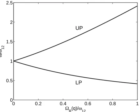
The values of the polariton frequencies, obtained diagonalizing Hamiltonian Hbos for different values of ΩR(q)/ω12 are shown in Fig. 2.2. From Eq. 2.2 we

see that the annihilation operator of a polariton is a linear combination of an-nihilation and creation operators of intersubband excitations and microcavity photons. The fact of having here both creation and annihilation operators is of fundamental importance. It is easy to verify that if _{|0i is the ground state}

38 Chapter 2. Quantum vacuum radiation phenomena 0 0.2 0.4 0.6 0.8 1 0 0.5 1 1.5 2 2.5 UP LP Ω_R(q)/ω 12 ω / ω 12

Figure 2.2: Normalized polariton frequencies ωLP,q/ω12 and ωU P,q/ω12 as a

function of ΩR(q)/ω12. The calculation has been performed with q such that

ωcav(q) + 2D(q) = ω12. See Ref. [25].

for the uncoupled microcavity-quantum wells system, defined by the relation aq|0i = bq|0i = 0, then pj,q|0i 6= 0. That is the ground state of the coupled

system is different from the one of the uncoupled system. If instead of Hamil-tonian Hbos we would have used the bosonic RWA Hamiltonian of Section 1.4.4

(that is Hbos without terms composed of two annihilation or two creation

op-erators ), annihilation and creation opop-erators would have been decoupled. In that case we would have pj,q|0i = 0. Antiresonant terms, which are relevant in the ultra-strong coupling regime, change the quantum ground state. The

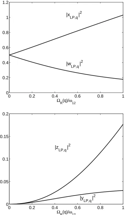
squared norm of the coefficients of the Hopfield-Bogoliubov transformation in Eq. 2.2 are shown in Fig. 2.3. Only in the ultra-strong coupling regime, y and z coefficients, that couple annihilation and creation operators, have non-negligible values. We thus introduce the polaritonic vacuum state|Gi, defined by pj,q|Gi = 0. From Eq. 2.2 we can calculate the expectation value of the

number of photons in this state

2.2. Quantum vacuum radiation as ultra-strong coupling effect 39 0 0.2 0.4 0.6 0.8 1 0 0.2 0.4 0.6 0.8 1 1.2 Ω_R(q)/ω 12 |x LP,q | 2 |w LP,q | 2 0 0.2 0.4 0.6 0.8 1 0 0.05 0.1 0.15 0.2 Ω_R(q)/ω 12 |z LP,q | 2 |y LP,q | 2

Figure 2.3: Mixing fractions for the Lower Polariton (LP) mode as a function of ΩR(q)/ω12. The calculation has been performed with q such that ωcav(q) +

2D(q) = ω12. The Upper Polariton (UP) fractions (not shown) are simply

|wU P,q| = |xLP,q|, |xU P,q| = |wLP,q|, |yU P,q| = |zLP,q|, |zU P,q| = |yLP,q|. See Ref.

40 Chapter 2. Quantum vacuum radiation phenomena This quantity can be quickly estimated from Fig. 2.3. In the ground state of the polaritonic system there is a finite population of virtual photons. These photons are virtual because, in absence of any time-dependent perturbation, they cannot escape from the cavity.

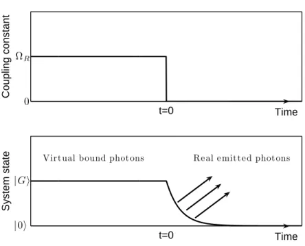
Now we can imagine a gedanken experiment in which our system is prepared in its ground state _{|Gi and in some way, at the time t = 0, we completely and} instantly switch off the light-matter interaction (see Fig. 2.4). Being the change non-adiabatic the system will be at the time t = 0+_{, still in the state}

|Gi, that now it is not anymore the ground state. Therefore, it is now an excited state and contains a finite and real photon population. Supposing the system coupled to an external reservoir, it will relax to its real ground state_|0i, emitting the exceeding energy as quantum vacuum radiation. A non-adiabatic change of the light-matter coupling can thus lead to the emission of photons out of the vacuum. Following Ref. [25] we can give a rough estimate of the number of emitted photons in this gedanken experiment, supposing that all the virtual photons are emitted outside the cavity. The number of photon states (per unit area) in the two dimensional momentum volume d2_{q is simply}

d2_q/(2π)2_{. Hence the differential density of photons (per unit area) in the two}

dimensional momentum volume d2_{q is}

dρphot=

d2_q

(2π)2hG|a †

qaq|Gi, (2.5)

where the photon number _hG|a†

qaq|Gi in the ground state is given by Eq. 2.4.

Rewriting Eq. 2.5 as a function of the propagation angle θ (q(θ) = qztan(θ))

we find that, for the resonance angle such that ωcav(q(θres)) + 2D(q) = ω12 we

have

dρphot

dθ = ω2

12ǫr

2πc2 tan(θres)hG|a†qaq|Gi. (2.6)

To give a numerical application of Eq. 2.6, we can consider the following values, taken from Ref. [37]: ~ω12 = 113 meV, a resonance angle θres = 65◦

and ~ΩR,q(θres) = 10 meV. For these parameters, Eq. 2.6 gives the differential

photon density dρphot

dθ ≃ 2.3 × 10

9_m−2_rad−1_{. We will use this reference value}

later as useful benchmark to test the theory and numerical methods developed in the following sections.

2.2. Quantum vacuum radiation as ultra-strong coupling effect 41 Time t=0 Coupling constant ΩR 0 Time t=0 System state |Gi |0i

Virtual bound photons Re al e mitte d photons

Figure 2.4: Pictorical representation of the gedanken experiment discussed in Section 2.2. The system is initially prepared in its ground state _{|Gi, with a} vacuum Rabi frequency ΩR(q). At the time t = 0, the light-matter coupling

is completely and abruptly switched off. Being the change non-adiabatic, the system at the time t = 0+ _{is still in the state|Gi, that now is not anymore the}

ground state and has thus (by definition) an energy bigger than the ground state. It will relax to its new ground state|0i (the standard vacuum), emitting the exceeding energy as quantum vacuum radiation.

42 Chapter 2. Quantum vacuum radiation phenomena

2.3

Formal theory

The gedanken experiment presented in the previous section showed us that we have to expect the emission of photons when the coupling constant is non-adiabatically modulated in time. In order to fully grasp the problem, we have to build up a quantitative theory capable of calculating the emitted radiation for an arbitrary time modulation of the coupling constant ΩR(q)(t), accounting

for the coupling with the environment. We need to consider the coupling of the system with an environment for a two-fold reason. On one side the intra-cavity fields, both matter and light, are not observable by themselves. What we can observe are the photons that leak out of the cavity due to the non-perfect reflectivity of the mirrors. On the other side the environment causes fluctuation and dissipation phenomena we have to consider in order to quantitatively model a real experiment.

We will consider a generic time varying vacuum Rabi frequency, composed of a fixed as well as a time dependent part:

ΩR(q, t) = ¯ΩR(q) + ΩmodR,q(t). (2.7)

We can take care of the coupling to the environment by using a generalized quantum Langevin formalism. All the details of the derivation can be found in Appendix B. The important point is that we can trace out the environment and obtain a self consistent quantum Langevin equation for the intra-cavity fields aq and bq only. The effect of the environment will all be contained in a causal

memory kernel (making the dynamics non-Markovian) and in a Langevin force term due to the environment-induced fluctuations. The Langevin equations for the system thus read

daq dt = − i ~[aq, Hbos]− Z dt′_Γ cav,q(t− t′)aq(t′) + Fcav,q(t), (2.8) dbq dt = − i ~[bq, Hbos]− Z dt′Γ12,q(t− t′)bq(t′) + F12,q(t),

where Γcav,q(t) and Γ12,q(t) are the memory kernels associated with the cavity

photon and matter fields and Fcav,q(t) and F12,q(t) are the respective Langevin

force operators. Real and imaginary parts of Γcav,q(t) and Γ12,q(t) are linked by

Kramers-Kroning relations, the real parts give an effective damping while the imaginary parts cause an energy shift due to the interactions. The expression of these quantities as a function of the environment parameters can be found in Appendix B. What is important to know here is that the real part of the

2.3. Formal theory 43 Fourier transform of the memory kernels ˜Γcav,q(ω) and ˜Γ12,q(ω) are directly

linked with the density of states in the environment with energy ~ω. Having the excitation modes in the environment all a positive energy we have

ℜ(˜Γcav,q(ω < 0)) =ℜ(˜Γ12,q(ω < 0)) = 0. (2.9)

In other words, the damping occurs only at positive frequencies. In order to solve this system of equations it is useful to pass in Fourier space in order to get rid of the convolution product due to the non-Markovian dynamics. Anyway the resulting equations will not be local in frequency, because of the time dependency of the vacuum Rabi frequency. It is convenient to define the following vectors for the Fourier transformed intra-cavity fields and Langevin forces: ˜ar q(ω)≡      ˜ aq(ω) ˜bq(ω) ˜a†_−q(−ω) ˜b† −q(−ω)      , F˜r_q(ω)_≡      ˜ Fcav,q(ω) ˜ F12,q(ω) ˜ F_cav,−q† (−ω) ˜ F_12,−q† (−ω)      . (2.10) We will moreover introduce two different Hopfield 4 × 4 matrices. The first, M_q,ω, groups all the time independent terms and the second, Mmod

q,ω , all the

terms due to the time-modulation of the vacuum Rabi frequency : M_q,ω =     

ωcav(q) + 2D(q)− ω − i˜Γcav,q(ω) ΩR(q)

ΩR(q) ω12− ω − i˜Γ12,q(ω) −2D(q) −ΩR(q) −ΩR(q) 0 (2.11) 2D(q) ΩR(q) ΩR(q) 0

−ωcav(q)− 2D(q) − ω − i˜Γ∗cav,q(−ω) −ΩR(q)

−ΩR(q) −ω12− ω − i˜Γ∗12,q(−ω)      , Mmod_q,ω =      2 ˜Dq(ω) Ω˜modR,q (ω) 2 ˜Dq(ω) Ω˜modR,q (ω) ˜ Ωmod R,q(ω) 0 Ω˜modR,q (ω) 0 −2 ˜Dq(ω) −˜ΩmodR,q (ω) −2 ˜Dq(ω) −˜ΩmodR,q (ω) −˜Ωmod R,q (ω) 0 −˜ΩmodR,q (ω) 0      . (2.12)

44 Chapter 2. Quantum vacuum radiation phenomena In this way the Fourier transform of the system in Eq. B.8, can be written in the simple matricial form:

Z ∞ −∞ dω′X s (Mrs_q,ω′δ(ω− ω′) + M mod rs q,ω−ω′)˜a s_(ω′₎ q =−i˜Frq(ω). (2.13)

We can see explicitly from Eq. 2.13 that the Mmod

q,ω matrix containing the

time modulation of the vacuum Rabi frequency couples different frequencies between them, making the system of equations nonlocal in frequency space. If we define

Mrs_q (ω, ω′)≡ Mrs

q,ω′δ(ω− ω′) + Mmod rs_q,ω−ω′, (2.14)

we can rewrite Eq. 2.13 in a more compact form: Z ∞

−∞

dω′X

s

Mrs_q (ω, ω′)˜as_q(ω′) =_−i˜Fr_q(ω). (2.15) In the following we will call Grs

q (ω, ω′) the inverse of Mrsq (ω, ω′). By definition

Z ∞

−∞

dω′X

s

Grs_q (ω, ω′)Mst_q(ω′, ω′′)_{≡ δ}rtδ(ω− ω′′). (2.16)

We can thus formally solve Eq. 2.15 as: ˜ar q(ω) =−i Z ∞ −∞ dω′X s Grs_q (ω, ω′_)˜Fs q(ω′). (2.17)

Therefore, we have solved, at least formally, the problem of calculating the intra-cavity photon field with an arbitrary time modulation of the vacuum Rabi frequency, fully accounting for the coupling with the environment. Now we would like to calculate the field emitted outside the cavity. As shown in Appendix A, the spectrum of the photonic field emitted outside the cavity can be calculated as a function of the intra-cavity photonic field ˜aq(ω) (supposing

the extra-cavity field initially in its vacuum state) as Sq(ω) =

1

πℜ(˜Γcav,q(ω))h˜a

†

q(ω)˜aq(ω)i. (2.18)

Inserting Eq. 2.17 into Eq. 2.18 we obtain: Sq(ω) = 1 πℜ(˜Γcav,q(ω)) Z ∞ −∞ Z ∞ −∞ dωdω′X rs G∗1r_q (ωq,q, ω)G1sq (ωq,q, ω′)h˜F†q(ω) r_F˜ q(ω′)si. (2.19)

2.4. Numerical results 45 In Appendix B we calculated the average values for quadratic forms of Langevin forces as

h˜F†q(ω)rF˜q(ω′)si = 4πδ(ω − ω′)δr,s[δr,3ℜ(˜Γcav,−q(−ω)) + δr,4ℜ(˜Γ12,−q(−ω))].

(2.20) Exploiting Eqs. 2.19 and 2.20, we can put the result in its final form:

Sq(ω) = 4ℜ(˜Γcav,q(ω))

Z ∞

−∞

dω′_|G13_q (ω, ω′)_|2_ℜ(˜Γcav,q(−ω′))

+ _|G14_q(ω, ω′)_|2_ℜ(˜Γ12,q(−ω′)). (2.21)

It is interesting to notice that if we have no modulation Mrs

q (ω, ω′) is

pro-portional to δ(ω _{− ω}′_{) and so is its inverse G}

q. Eq. 2.21 then tells us that

Sq(ω) ∝ ℜ(˜Γcav,q(ω))ℜ(˜Γcav,q(−ω)). From Eq. 2.9 we thus conclude that

Sq(ω) = 0. This shows explicitly that, as expected, in absence of any modula-tion no photon is emitted out of the cavity.

2.4

Numerical results

In order to obtain the spectrum of emitted radiation, given by Eq. 2.21, we need to numerically calculate Grs

q (ω, ω′). This does not pose any major

technical problem as it is easy to verify that Eq. 2.16 defines Grs

q (ω, ω′) as the

inverse of the linear operator Mrs

q(ω, ω′). It is thus sufficient to discretize the

frequency space on a grid of Nω points, write down Mqas a 4Nω×4Nω matrix

and invert it.

At first, we applied our theory to the case of a periodic sinusoidal modu-lation, in order to be able to study the emission spectra as a function of only two parameters, the amplitude of the modulation ∆ΩR(q) and its frequency

ωmod. We thus consider a vacuum Rabi frequency of the form:

ΩR(q, t) = ¯ΩR(q) + ∆ΩR(q) sin(t). (2.22)

Being the modulation periodic (and thus acting for an infinite time) the rel-evant quantity to consider is not the spectral density of emitted photons per mode Sq(ω) but the spectral density of emitted photons per mode and per unit

time dSq(ω)/dt. Integrating it over the whole frequency range we can find the

total number of emitted photons per mode per unit time dNqout/dt =

Z ∞

−∞

dSq(ω)

46 Chapter 2. Quantum vacuum radiation phenomena This is the steady quantum vacuum fluorescence rate. Predictions for the rate dNout

q /dt of emitted photons as a function of the modulation frequency ωmod

(in units of ω12) are shown in Fig. 2.5 for the resonant case ω12 = ωcav(q) +

2D(q) for which the emission is the strongest. Thanks to the ultra-strong coupling regime, the emission intensity however has a moderate q dependence, remaining important over a wide anticrossing region. For the sake of simplicity, a frequency-independent damping rate has been consideredℜ{˜Γcav,q(ω > 0)} =

ℜ{˜Γ12,q(ω > 0)} = Γ, and the imaginary part has been consistently determined

via the Kramers-Kronig relations [33]. Values inspired from recent experiments [24, 67, 68] have been used for the cavity parameters. Representative results are shown in Fig. 2.5. The structures in the integrated spectrum shown in Fig. 2.5 can be identified as resonance peaks when the modulation is phase-matched. We can effectively consider the dynamical Casimir effect as a parametric

0.5 1 1.5 2 2.5 3 3.5 10−6 10−5 10−4 10−3 10−2 10−1 100 ω_mod / ω 12 (dN q out /dt) / ω 12 A B C

Figure 2.5: Rate of emitted photons dNout

q /dt (in units of ω12) as a function

of the normalized modulation frequency ωmod/ω12. Parameters: (ωcav(q) +

2D(q))/ω12 = 1, Γ/ω12 = 0.025, ¯ΩR(q)/ω12 = 0.2, ∆ΩR(q)/ω12 = 0.04. The

letters A, B and C indicate three different resonantly enhanced processes. excitation of the quantum vacuum. As usual for parametric processes [69],

2.4. Numerical results 47

Figure 2.6: On the left are plotted the spectral densities of emitted photons (arb. u.) for the processes A, B and C of Fig. 2.5. On the right there is a schematic representation of the three phase-matched parametric processes involved.