arXiv:1904.09145v2 [math.PR] 8 Apr 2020
Universality for critical KCM:
infinite number of stable directions
Ivailo Hartarsky
∗,1,2, Laure Marêché
†,3, and Cristina Toninelli
‡,21
DMA UMR 8553, École Normale Supérieure CNRS, PSL Research University 45 rue d’Ulm, 75005 Paris, France
2
CEREMADE UMR 7534, Université Paris-Dauphine CNRS, PSL Research University
Place du Maréchal de Lattre de Tassigny, 75775 Paris Cedex 16, France
3
LPSM UMR 8001, Université Paris Diderot CNRS, Sorbonne Paris Cité
75013 Paris, France
April 9, 2020
Abstract
Kinetically constrained models (KCM) are reversible interacting particle systems on Zd with continuous-time constrained Glauber dynamics. They are a natural
non-monotone stochastic version of the family of cellular automata with random initial state known as U-bootstrap percolation. KCM have an interest in their own right, owing to their use for modelling the liquid-glass transition in condensed matter physics.
In two dimensions there are three classes of models with qualitatively different scal-ing of the infection time of the origin as the density of infected sites vanishes. Here we study in full generality the class termed ‘critical’. Together with the companion paper by Martinelli and two of the authors [20] we establish the universality classes of critical KCM and determine within each class the critical exponent of the infection time as well as of the spectral gap. In this work we prove that for critical models with an infinite number of stable directions this exponent is twice the one of their bootstrap percolation counterpart. This is due to the occurrence of ‘energy barriers’, which determine the dominant behaviour for these KCM but which do not matter for the monotone boot-strap dynamics. Our result confirms the conjecture of Martinelli, Morris and the last author [26], who proved a matching upper bound.
MSC2010: Primary 60K35; Secondary 82C22, 60J27, 60C05
Keywords: Kinetically constrained models, bootstrap percolation, universality, Glauber dynamics, spectral gap.
1
Introduction
Kinetically constrained models (KCM) are interacting particle systems on the integer lat-tice Zd, which were introduced in the physics literature in the 1980s by Fredrickson and
Andersen [16] in order to model the liquid-glass transition (see e.g. [17, 31] for reviews), a major and still largely open problem in condensed matter physics [5]. A generic KCM is a continuous-time Markov process of Glauber type characterised by a finite collection U of fi-nite nonempty subsets of Zdzt0u, its update family. A configuration ω is defined by assigning
to each site xP Zd an occupation variable ω
x P t0, 1u, corresponding to an empty or occupied
site respectively. Each site x P Zd waits an independent, mean one, exponential time and
then, iff there exists U P U such that ωy “ 0 for all y P U ` x, site x is updated to empty with
probability q and to occupied with probability 1´q. Since each U P U is contained in Zdzt0u,
the constraint to allow the update does not depend on the state of the to-be-updated site. As a consequence, the dynamics satisfies detailed balance w.r.t. the product Bernoulli(1´ q) measure, µ, which is therefore a reversible invariant measure. Hence the process started at µis stationary.
Both from a physical and from a mathematical point of view, a central issue for KCM is to determine the speed of divergence of the characteristic time scales when q Ñ 0. Two key quantities are: (i) the relaxation time Trel, i.e. the inverse of the spectral gap of the
Markov generator (see Definition 2.5) and (ii) the mean infection time Epτ0q, i.e. the mean
over the stationary process started at µ of the first time at which the origin becomes empty. Several works have been devoted to the study of these time scales for some specific choices of the constraints [2, 9, 12, 13, 25, 27] (see also [17] section 1.4.1 for a non exhaustive list of references in the physics literature). These results show that KCM exhibit a very large variety of possible scalings depending on the update family U. A question that naturally emerges, and that has been first addressed in [26], is whether it is possible to group all possible update families into distinct universality classes so that all models of the same class display the same divergence of the time scales.
Before presenting the results and the conjectures of [26], we should describe the key connection of KCM with a class of discrete monotone cellular automata known as U-bootstrap percolation (or simply bootstrap percolation) [8]. For U-bootstrap percolation on Zd, given
an update family U and a set At of sites infected at time t, the infected sites in At remain
infected at time t` 1, and every site x becomes infected at time t ` 1 if the translate by x of one of the sets in U is contained in At. The set of initial infections A is chosen at
random with respect to the product Bernoulli measure with parameter q P r0, 1s, which identifies with µ: for every x P Zd we have µpx P Aq “ q. One then defines the critical
probability qc`Zd,U˘ to be the infimum of the q such that with probability one the whole
lattice is eventually infected, namely Ť
tě0At “ Zd. A key time scale for this dynamics is
the first time at which the origin is infected, τBP. In order to study this infection time for
models on Z2, the update families were classified by Bollobás, Smith and Uzzell [8] into three
universality classes: supercritical, critical and subcritical, according to a simple geometric criterion (see Definition 2.1). In [8] they proved that qc`Z2,U
˘
“ 0 if U is supercritical or critical, and it was proved by Balister, Bollobás, Przykucki and Smith [4] that qc`Z2,U
˘ ą 0 if U is subcritical. For supercritical update families, [8] proved that τBP “ q´Θp1q w.h.p.
as q Ñ 0, while in the critical case τBP “ exppq´Θp1qq. The result for critical families was
later improved by Bollobás, Duminil-Copin, Morris and Smith [7], who identified the critical exponent α“ αpUq such that τBP“ exppq´α`op1qq.
the empty sites with infected sites, a first basic observation is that the clusters of sites that will never be infected in the U-bootstrap percolation correspond to clusters of sites which are occupied and will never be emptied under the KCM dynamics. A natural issue is whether there is a direct connection between the infection mechanism of bootstrap percolation and the relaxation mechanism for KCM, and, more precisely, whether the scaling of Trel and Epτ0q
is connected to the typical value of τBP when the law of the initial infections is µ. It is not
difficult to establish that µpτBPq provides a lower bound for Epτ0q and Trel(see [27, Lemma 4.3]
and (10)), but in general, as we will explain, this lower bound does not provide the correct behaviour.
In [26], Martinelli, Morris and the last author proposed that the supercritical class should be refined into unrooted supercritical and rooted supercritical models in order to capture the richer behavior of KCM. For unrooted models the scaling is of the same type as for bootstrap percolation, Trel „ Epτ0q “ q´Θp1q as q Ñ 0 [26, Theorem 1(a)]
1
, while for rooted models the divergence is much faster, Epτ0q „ Trel“ eΘpplog qq
2
q (see [26, Theorem 1(b)] for the upper
bound and [25, Theorem 4.2] for the lower bound).
Concerning the critical class, the lower bound with µpτBPq mentioned above and the
re-sults of [8] on bootstrap percolation imply that Trel and Epτ0q diverge at least as exppq´Θp1qq.
In [26, Theorem 2] an upper bound of the same form was established and a conjecture [26, Conjecture 3] was put forward on the value of the critical exponent ν such that both Epτ0q
and Trel scale as expp| log q|Op1q{qνq, with ν in general different from the exponent of the
corresponding bootstrap percolation process. Furthermore, a toolbox was developed for the study of the upper bounds, leading to upper bounds matching this conjecture for all mod-els. The main issue left open in [26] was to develop tools to establish sharp lower bounds. A first step in this direction was done by Martinelli and the last two authors [25] by an-alyzing a specific critical model known as the Duarte model for which the update family contains all the 2-elements subsets of the North, South and West neighbours of the origin. Theorem 5.1 of [25] establishes a sharp lower bound on the infection and relaxation times for the Duarte KCM that, together with the upper bound in [26, Theorem 2(a)], proves
EDuarte
pτ0q “ exp pΘpplog qq4{q2qq as q Ñ 0, and the same result holds for Trel. The divergence
is again much faster than for the corresponding bootstrap percolation model, for which it holds τBP “ eΘpplog qq
2
{qq w.h.p as q Ñ 0 [30] (see also [6], from which the sharp value of
the constant follows), namely the critical exponent for the Duarte KCM is twice the critical exponent for the Duarte bootstrap percolation.
Both for Duarte and for supercritical rooted models, the sharper divergence of time scales for KCM is due to the fact that the infection time of KCM is not well approximated by the infection mechanism of the monotone bootstrap percolation process, but is instead the result of a much more complex infection/healing mechanism. Indeed, visiting regions of the configuration space with an anomalous amount of empty sites is heavily penalised and requires a very long time to actually take place. The basic underlying idea is that the dominant relaxation mechanism is an like dynamics for large droplets of empty sites. Here East-like means that the presence of an empty droplet allows to empty (or fill) another adjacent droplet but only in a certain direction (or more precisely in a limited cone of directions). This is reminiscent of the relaxation mechanism for the East model, a prototype one-dimensional KCM for which x can be updated iff x´ 1 is empty, thus a single empty site allows to create/destroy an empty site only on its right (see [15] for a review on the East model). For supercritical rooted models, the empty droplets that play the role of the single empty sites
1
For the lower bound of Trel one does not need to use the boostrap percolation results, as Trel ě
q´ minU PU|U|{|U| by plugging the test function
1tω
for East have a finite (model dependent) size, hence an equilibrium density qeff “ qΘp1q. For
the Duarte model, droplets have a size that diverges as ℓ“ | log q|{q and thus an equilibrium density qeff “ qℓ “ e´plog qq
2{q
. Then a (very) rough understanding of the results of [25, 26] is obtained by replacing q with qeff in the time scale for the East model T
East
rel “ eΘpplog qq
2
q[2]. The
main technical difficulty to translate this intuition into a lower bound is that the droplets cannot be identified with a rigid structure. In [25] this difficulty for the Duarte model was overcome by an algorithmic construction that allows to sequentially scan the system in search of sets of empty sites that could (without violating the constraint) empty a certain rigid structure. These are the droplets that play the role of the empty sites for the East dynamics.
In [26] all critical models which have an infinite number of stable directions (see Section 2.1), of which the Duarte model is but one example, were conjectured to have a critical exponent ν “ 2α, with α “ αpUq the critical exponent of the corresponding bootstrap percolation dynamics (defined in Definition 2.2). The heuristics is the same as for the Duarte model, the only difference being that droplets would have in general size ℓ“ | log q|Op1q{qα.
However, the technique developed in [25] for the Duarte model relies heavily on the specific form of the Duarte constraint and in particular on its oriented nature2
, and it cannot be extended readily to this larger class.
In this work, together with the companion paper by Martinelli and two of the authors [20], we establish in full generality the universality classes for critical KCM, determining the critical exponent for each class.
Here we treat all choices of U for which there is an infinite number of stable directions and prove (Theorem 2.8) a lower bound for Trel and Epτ0q that, together with the matching
upper bound of [26, Theorem 2], yields
Epτ0q “ e| log q|
Op1q{q2α
for q Ñ 0 and the same result for Trel. Our technique is somewhat inspired by the algorithmic
construction of [25], however, the nature of the droplets which move in an East-like way is here much more subtle, and in order to identify them we construct an algorithm which can be seen as a significant improvement on the α-covering and u-iceberg algorithms developed in the context of bootstrap percolation [7].
In the companion paper [20] we prove for the complementary class of models, namely all critical models with a finite number of stable directions, an upper bound that (together with the lower bound from bootstrap percolation) yields instead
Epτ0q “ e| log q|
Op1q{qα
for qÑ 0 and the same result for Trel.
A comparison of our results with Conjecture 3 of [26] is due. The class that we consider here is, in the notation of [26], the class of models with bilateral difficulty β“ 8, hence belong to the α-rooted class defined therein. Therefore, our Theorem 2.8 proves Conjecture 3(a) in this case. We underline that it is not a limitation of our lower bound strategy that prevents us from proving Conjecture 3(a) for the other α-rooted models, namely those with 2αď β ă 8. Indeed, as it is proven in the companion paper [20], in this case the conjecture of [26] is not correct, since it did not take into account a subtle relaxation mechanism which allows to recover the same critical exponent as for the bootstrap percolation dynamics.
2
Note that, since the Duarte update rules contain only the North, South and West neighbours of the origin, the constraint at a site x does not depend on the sites with abscissa larger than the abscissa of x.
The plan of the paper is as follows. In Section 2 we develop the background for both KCM and bootstrap percolation needed to state our result, Theorem 2.8. In Section 3 we give a sketch of our reasoning and highlight the important points. In Section 4 we gather some preliminaries and notation. Section 5 is the core of the paper — there we define the central notions and establish their key properties, culminating in the Closure Proposition 5.20. In Section 6 we establish a connection between the KCM dynamics and an East dynamics and use this to wrap up the proof of Theorem 2.8. Finally, in Section 7 we discuss some open problems.
2
Models and background
2.1
Bootstrap percolation
Before turning to our models of interest, KCM, let us recall recent universality results for the intimately connected bootstrap percolation models in two dimensions. U-bootstrap per-colation (or simply bootstrap perper-colation) is a very general class of monotone transitive local cellular automata on Z2 first studied in full generality by Bollobás, Smith and Uzzell [8]. Let
U, called update family, be a finite family of finite nonempty subsets, called update rules, of Z2zt0u. Let A, called the set of initial infections, be an arbitrary subset of Z2. Then
the U-bootstrap percolation dynamics is the discrete time deterministic growth of infection defined by A0 “ A and, for each t P N,
At`1 “ AtY tx P Z2: D U P U, U ` x Ă Atu.
In other words, at any step each site becomes infected if a rule translated at it is already fully infected, and infections never heal. We define the closure of the set A by rAs “ Ťtě0At and
we say that A is stable when rAs “ A. The set of initial infections A is chosen at random with respect to the product Bernoulli measure µ with parameter qP r0, 1s: for every x P Z2
we have µpx P Aq “ q.
Arguably, the most natural quantity to consider for these models is the typical (e.g. mean) value of τBP, the infection time of the origin.
The combined results of Bollobás, Smith and Uzzell [8] and Balister, Bollobás, Przykucki and Smith [4] yield a pre-universality partition of all update families into three classes with qualitatively different scalings of the median of the infection time as qÑ 0. In order to define this partition we will need a few definitions.
For any unitary vector u P S1 “ tz P R2: }z} “ 1u (} ¨ } denotes the Euclidean norm
in R2) and any vector x P R2 we denote H
upxq “ ty P R2: xu, y ´ xy ă 0u — the open
half-plane directed by u passing through x. We also set Hu “ Hup0q. We say that a direction
uP S1 is unstable (for an update family U) if there exists U P U such that U Ă H
u and stable
otherwise. The partition is then as follows.
Definition 2.1 (Definition 1.3 of [8]). An update family U is
• supercritical if there exists an open semi-circle of unstable directions,
• critical if it is not supercritical, but there exists an open semi-circle with a finite number of stable directions,
The main result of [8] then states that in the supercritical case τBP “ q´Θp1q with high
probability as q Ñ 0, while in the critical one τBP “ exppq´Θp1qq. The final justification of
the partition in Definition 2.1 was given by Balister, Bollobás, Przykucki and Smith [4] who proved that the origin is never infected with positive probability for subcritical models for qą 0 sufficiently small, i.e. qc`Z2,U
˘
ą 0 if U is subcritical. From the bootstrap percolation perspective supercritical models are rather simple, while subcritical ones remain very poorly understood (see [19]). Nevertheless, most of the non-trivial models considered before the introduction of U-bootstrap percolation, including the 2-neighbour model (see [1, 22] for further results), fall into the critical class, which is also the focus of our work.
Significantly improving the result of [8], Bollobás, Duminil-Copin, Morris and Smith [7] found the correct exponent determining the scaling of τBP for critical families. Moreover,
they were able to find log τBP up to a constant factor. To state their results we need the
following crucial notion.
Definition 2.2 (Definition 1.2 of [7]). Let U be an update family and uP S1 be a direction.
Then the difficulty of u, αpuq, is defined as follows. • If u is unstable, then αpuq “ 0.
• If u is an isolated stable direction (isolated in the topological sense), then αpuq “ mintn P N: DK Ă Z2,|K| “ n, |rZ2X pH
uY KqszHu| “ 8u, (1)
i.e. the minimal number of infections allowing Hu to grow infinitely.
• Otherwise, αpuq “ 8. We define the difficulty of U by
αpUq “ inf
CPCsupuPCαpuq, (2)
where C “ tHuX S1: uP S1u is the set of open semi-circles of S1.
It is not hard to see (Theorem 1.10 of [8], Lemma 2.6 of [7]) that the set of stable directions is a finite union of closed intervals of S1 and that (Lemmas 2.7 and 2.10 of [7]) (1)
also holds for unstable and strongly stable directions, that is directions in the interior of the set of stable directions (but not for semi-isolated stable directions i.e. endpoints of non-trivial stable intervals). Furthermore (see [7, Lemma 2.7], [8, Lemma 5.2]), 1 ď αpuq ă 8 if and only if u is an isolated stable direction, so that U is critical if and only if 1ď αpUq ă 8. As a final remark we recall that, contrary to determining whether an update family is critical, finding αpUq is a NP-hard question [21].
We are now ready to describe the universality results. A weaker form of the result of [7] is that τBP“ exppq´αpU q`op1qq with high probability as q Ñ 0. For the full result however, we
need one last definition.
Definition 2.3. A critical update family U is balanced if there exists a closed semi-circle C such that maxuPCαpuq “ αpUq and unbalanced otherwise.
Then [7] provides that for balanced models τBP “ exppΘp1q{qαpU qq with high probability
as qÑ 0, while for unbalanced ones τBP “ exppΘpplog qq2q{qαpU qq. These are the best general
estimates currently known. We refer to [28, 29] for recent surveys on these results as well as on sharper results for some specific models.
2.2
Kinetically constrained models
Returning to KCM, let us first define the general class of KCM introduced by Cancrini, Martinelli, Roberto and the last author [9] directly on Z2. Fix a parameter q P r0, 1s and an
update family U as in the previous section. The corresponding KCM is a continuous-time Markov process on Ω“ t0, 1uZ2
which can be informally defined as follows. A configuration ω is defined by assigning to each site xP Z2 an occupation variable ω
x P t0, 1u corresponding
to an empty (or infected ) and occupied (or healthy) site respectively. Each site waits an independent exponentially distributed time with mean 1 before attempting to update its occupation variable. At that time, if the configuration is completely empty on at least one update rule translated at x, i.e. ifDU P U such that ωy “ 0 for all y P U ` x, then we perform
a legal update or legal spin flip by setting ωx to 0 with probability q and to 1 with probability
1´ q. Otherwise the update is discarded. Since the constraint to allow the update never depends on the state of the to-be-updated site, the product measure µ is a reversible invariant measure and the process started at µ is stationary. More formally, the KCM is the Markov process on Ω with generator L acting on local functions f : ΩÞÑ R as
pLfqpωq “ ÿ
xPZ2
cxpωq pµxpfq ´ fq pωq, (3)
for any ω P Ω, where µxpfq denotes the average of f when the occupation variable at x has
law Berp1 ´ qq and the other occupation variables are set to tωyuy‰x, and cx is the indicator
function of the event that there exists U P U such that U ` x is completely empty, i.e. ωU`x ” 0. We refer the reader to chapter I of [24], where the general theory of interacting
particle systems is detailed, for a precise construction of the Markov process and the proof that L is the generator of a reversible Markov processtωptqutě0 on Ω with reversible measure
µ.
The corresponding Dirichlet form is defined as Dpfq “ ÿ
xPZ2
µ`cxVarxpfq˘, (4)
where Varxpfq denotes the variance of the local function f with respect to the variable ωx
conditionally ontωyuy‰x. The expectation with respect to the stationary process with initial
distribution µ will be denoted by E“ Eq,U
µ . Finally, given a configuration ω P Ω and a site
x P Z2, we will denote by ωx the configuration obtained from ω by flipping site x, namely
by setting pωxq
x “ 1 ´ ωx and pωxqy “ ωy for all y ‰ x. For future use we also need the
following definition of legal paths, that are essentially sequences of configurations obtained by successive legal updates.
Definition 2.4 (Legal path). Fix an update family U, then a legal path γ in Ω is a finite sequence γ “ `ωp0q, . . . , ωpkq˘ such that, for each iP t1, . . . , ku, the configurations ωpi´1q and
ωpiqdiffer by a legal (with respect to the choice of U) spin flip at some vertex v “ vpωpi´1q, ωpiqq.
As mentioned in Section 1, our goal is to prove sharp bounds on the characteristic time scales of critical KCM. Let us start by defining precisely these time scales, namely the re-laxation time Trel (or inverse of the spectral gap) and the mean infection time Epτ0q (with
respect to the stationary process).
Definition 2.5 (Relaxation time Trel). Given an update family U and q P r0, 1s, we say that
Cą 0 is a Poincaré constant for the corresponding KCM if, for all local functions f, we have Varµpfq “ µpf2q ´ µpfq2 ď C Dpfq. (5)
If there exists a finite Poincaré constant, we define
Trel “ Trelpq, Uq “ inf tC ą 0 : C is a Poincaré constantu .
Otherwise we say that the relaxation time is infinite.
A finite relaxation time implies that the reversible measure µ is mixing for the semigroup Pt“ etL with exponentially decaying time auto-correlations (see e.g. [3, Section 2.1]).
Definition 2.6 (Infection time τ0). The random time τ0 at which the origin is first infected
is given by
τ0 “ inf t ě 0 : ω0ptq “ 0(,
where we adopt the usual notation letting ω0ptq be the value of the configuration ωptq at the
origin, namely ω0ptq “ pωptqq0.
The East model We close this section by defining a specific example of KCM on Z, the East model of Jäckle and Eisinger [23], which will be crucial to understand our results (KCM on Z are defined in the same way as KCM on Z2). It is defined by an update family composed
by a single rule containing only the site to the left of the origin (´1). In other words, site x can be updated iff x´ 1 is empty. For this model both Trel and Epτ0q scale as exp
´
plog qq2
2 log 2
¯
as q Ñ 0, see [2, 9, 12]3
. One of the key ingredients behind this scaling is the following combinatorial result [32] (see [14, Fact 1] for a more mathematical formulation).
Proposition 2.7. Consider the East model ont1, . . . , Mu defined by fixing ω0 “ 0 at all time.
Then any legal path γ connecting the fully occupied configuration (namely ω s.t. ωx “ 1 for
all xP t1, . . . , Mu) to a configuration ω1 such that ω1
M “ 0 goes through a configuration with
at least rlog2pM ` 1qs empty sites.
This logarithmic ‘energy barrier’, to employ the physics jargon, and the fact that at equilibrium the typical distance to the first empty site is M “ Θp1{qq are responsible for the divergence of the time scales as roughly 1{qrlog2pM `1qs“ eΘpplog qq2q.
2.3
Result
In this paper we study critical KCM with an infinite number of stable directions or, equiva-lently, with a non-trivial interval of stable directions. Recall that E denotes the expectation with respect to the stationary KCM process.
Theorem 2.8. Let U be a critical update family with an infinite number of stable directions. Then there exists a sufficiently large constant C ą 0 such that
Epτ0q ě exp `1{ `Cq2αpU q˘˘ ,
as qÑ 0 and the same asymptotics holds for Trel.
3
Actually these references focus on the study of Trel. A matching upper bound for Epτ0q follows from (10).
The lower bound for Epτ0q follows easily from the lower bound for Ppτ0 ą tq with t “ exp plogpqq 2
{2 log 2q obtained in the proof of Theorem 5.1 of [11].
This theorem combined with the upper bound of Martinelli, Morris and the last author [26, Theorem 2(a)], determines the critical exponent of these models to be 2α in the sense of Corollary 2.9 below. We thus complete the proof of universality and Conjecture 3(a) of [26] for these models4
.
Corollary 2.9. Let U be a critical update family with an infinite number of stable directions. Then
q2αpU qlog Epτ0q “ p´ log qqOp1q
as qÑ 0 and the same holds for Trel.
Universality for the remaining critical models is proved in a companion paper by Martinelli and the first and third authors [20] and, in particular, Conjecture 3(a) of [26] is disproved for models other than those covered by Theorem 2.8. It is important to note that Theo-rem 2.8 significantly improves the best known results for all models with the exception of the recent result of Martinelli and the last two authors [25] for the Duarte model. Indeed, the previous bound had exponent α, and was proved via the general (but in this case far from optimal) lower bound with the mean infection time for the corresponding bootstrap percolation model [27, Lemma 4.3].
3
Sketch of the proof
In this section we outline roughly the strategy to derive our main result, Theorem 2.8. The hypothesis of infinite number of stable directions provides us with an interval of stable directions. We can then construct stable ‘droplets’ of shape as in Figure 3 (see Definitions 5.5 and 5.6), where we recall from Section 2.1 that a set is stable if it coincides with its closure. Thus, if all infections are initially inside a droplet, this will be true at any time under the KCM dynamics. The relevance and advantage of such shapes come from the fact that only infections situated to the left of a droplet can induce growth left. This is manifestly not feasible without the hypothesis of having an interval of stable directions. It is worth noting that these shapes, which may seem strange at first sight, are actually very natural and intrinsically present in the dynamics. Indeed, such is the shape of the stable sets for a representative model of this class – the modified 2-neighbour model with one (any) rule removed, that is the three-rule update family with rulestp´1, 0q, p0, 1qu,tp´1, 0q, p0, ´1qu,tp0, ´1q, p1, 0qu (it can also be seen as the modified Duarte model with an additional rule). The stable sets in this case are actually Young diagrams.
We construct a collection of such droplets covering the initial configuration of infections, so that it gives an upper bound on the closure. To do this, we devise an improvement of the α-covering algorithm of Bollobás, Duminil-Copin, Morris and Smith [7]. It is important for us not to overestimate the closure as brutally. Indeed, a key step and the main difficulty of our work is the Closure Proposition 5.20, which roughly states that the collections of droplets associated to the closure of the initial infections is equal to the collection for the initial infections. This is highly non-trivial, as in order not to overshoot in defining the droplets, one is forced to ignore small patches of infections (larger than the ones in [7]), which can possibly grow significantly when we take the closure for the bootstrap percolation process and especially so if they are close to a large infected droplet. In order to remedy this problem, we introduce a relatively intrinsic notion of ‘crumb’ (see Definition 5.1) such that
4
The conjecture involuntarily asks for a positive power of log q, which we do not expect to be systematically present (see Conjecture 7.1).
its closure remains one and does not differ too much from it. A further advantage of our algorithm for creating the droplets over the one of [7] is that it is somewhat canonical, with a well-defined unique output, which has particularly nice ‘algebraic’ description and properties (see Remark 5.10). Another notable difficulty we face is systematically working in roughly a half-plane (see Remark 5.21 for generalisations) with a fully infected boundary condition, but we manage to extend our reasoning to this setting very coherently.
Finally, having established the Closure Proposition 5.20 alongside standard and straight-forward results like an Aizenmann-Lebowitz Lemma 5.13 and an exponential decay of the probability of occurrence of large droplets (Lemma 5.15), we finish the proof via the follow-ing approach, inspired by the one developed by Martinelli and the last two authors [25] for the Duarte model. The key step here (see Section 6) is mapping the KCM legal paths to those of an East dynamics via a suitable renormalisation. Roughly speaking, we say that a renormalised site is empty if it contains a large droplet of infections. However, for the renor-malised configuration to be mostly invariant under the original KCM dynamics, we rather look for the droplets in the closure of the original set of infections instead. This is where the Closure Proposition 5.20 is used to compensate the fact that the closure of equilibrium is not equilibrium. In turn, this mapping together with the combinatorial result for the East model recalled in Section 2.2 (Proposition 2.7), yield a bottleneck for our dynamics corresponding to the creation of logp1{qeffq droplets, where 1{qeff is the equilibrium distance between two
empty sites in the renormalized lattice, and qeff „ e´1{q
α
. This provides for the time scales the desired lower bound qlogpqeffq
eff „ e1{q
2α
of Theorem 2.8. The last part of the proof follows very closely the ideas put forward in [25] for the Duarte model. However, in [25], there was no need to develop a subtle droplet algorithm since, owing to the oriented character of the Duarte constraint, droplets could simply be identified with some large infected vertical segments. It is also worth noting that, thanks to the less rigid notion of droplets that we develop in the general setting, some of the difficulties faced in [25] for Duarte are no longer present here.
4
Preliminaries and notation
Let us fix a critical update family U with an infinite number of stable directions for the rest of the paper. We will omit U from all notation, such as αpUq.
Directions The next lemma establishes that one can make a suitable choice of 4 stable directions, which we will use for all our droplets. At this point the statement should look very odd and technical, but it simply reflects the fact that we have a lot of freedom for the choice and we make one which will simplify a few of the more technical points in later stages. Nevertheless, this is to a large extent not needed besides for concision and clarity.
A direction uP S1 is called rational if tan uP Q Y t8u.
Lemma 4.1. There exists rational stable directions S “ tu1, u2, v1, v2u (see Figure 1) with
difficulty at least α such that
• The directions appear in couterclockwise order u1, u2, v1, v2.
• No uP S is a semi-isolated stable direction.
• u3´i belongs to the cone spanned by vi and ui for i P t1, 2u i.e. the strictly smaller
u1 u2 v1 1 v12 u1` π u2´ π 1 2 3
Figure 1: Illustration of Lemma 4.1 and its proof. Thickened arcs represent intervals of strongly stable directions. Solid dots repre-sent isolated and semi-isolated stable directions. The difficulties of the isolated stable directions are indicated next to them and yield that the difficulty of the model is α“ 2. The directions chosen in Lemma 4.1 are the solid vectors u1, u2, v1 “ v11 and a direction v2
in the strongly stable interval ending at v1
2 sufficiently close to v21.
Note that the definition of v1
2 (and v11) disregards stable directions
with difficulty smaller than α as present on the figure. • 0is contained in the interior of the convex envelope of S.
• Either u2 ă v1´ π{2 or u1 ą v2` π{2.
• pHu1 Y Hu2q X Z
2 is stable or, equivalently, EU P U, U Ă H
u1 Y Hu2. • the directions u1 “pu1` u2q{2, u11 “p3u1` u2q{4, u12 “pu1` 3u2q{4 are rational.
Proof. Since U has an infinite number of stable directions and they form a finite union of closed intervals with rational endpoints [8, Theorem 1.10], there exists a non-empty open interval I3 of stable directions. Further note that the set J of directions u such that there
exists a rule U P U and x P U with xx, uy “ 0 is finite, so one can find a non-trivial closed subinterval I2 Ă I3 which does not intersect J. The directions u
1and u2 will be chosen in I2,
which clearly implies that they are strongly stable and thus with infinite difficulty. Moreover, if there exists U P U with U Ă Hu1 Y Hu2, by stability of u2, we have U X pHu1zHu2q ‰ ∅,
which contradicts I2X J “ ∅.
Since U is critical it does not have two opposite strongly stable directions, so there is no strongly stable direction in I2 ` π. If there are any (isolated or semi-isolated) stable
directions in I2` π, we can further choose a non-trivial open subinterval I1 Ă I2, for which
this is not the case (there is a finite number of isolated and semi-isolated stable directions). Let π ą δ ą 0 be such that the angle between any two consecutive directions of difficulty at least α is at most π´ δ (it is well defined by (2)). We then choose a non-trivial closed subinterval I1 Ą I “ ru
1, u2s with u1 rational and u11 “ p3u1 ` u2q{4 rational and with
0ă u2´ u1 ă δ ă π. It easily follows from the sum and difference formulas for the tangent
function that u1, u1
2 and u2 are also rational.
Let
v11 “ maxtv P pu2, u1` πq: αpvq ě αu,
v12 “ mintv P pu2´ π, u1q: αpvq ě αu.
These both exist, since I` π does not contain stable directions, both pu2, u2` πq and pu1´
π, u1q contain directions with difficulty at least α by (2) and the set of such directions is
closed. If v1
1 is not semi-isolated, we set v1 “ v11 and similarly for v2. Otherwise, we choose a
rational strongly stable direction sufficiently close to v1
that this choice satisfies all the desired conditions. Indeed, all directions in S are stable non-semi-isolated rational with difficulty at least α and the last but one condition was already verified.
One does have that u1 is in the cone spanned by v2 and u2, which is implied by v2 P
pu2´ π, u1q and similarly for u2, so the third condition is also verified. If v12´ v11 ě π, then
there is an open half circle contained in pv1
1, v21q with no direction of difficulty at least α,
which contradicts (2), so v2´ v1 ă π and the same holds for u1´ v2, u2´ u1 and v1´ u2 by
the definition of v1
1 and v21, the fact that v1 and v2 are sufficiently close to them and the fact
that I was chosen smaller than π. Thus 0 is in the convex envelope of S.
Finally, if one has both v1´ u2 ď π{2 and u1´ v2 ď π{2, then one obtains v21 ´ v11 ą π ´ δ,
since I is smaller than δ. However, v1
1 and v21 are consecutive directions of difficulty at least
α, which contradicts the definition of δ.
Notation For the rest of the paper we fix directions S “ tu1, u2, v1, v2u as in Lemma 4.1
and assume without loss of generality that u2 ă v1´ π{2.
Let us fix large constants
1! C1 ! C21 ! C2 ! C3 ! C41 ! C4 ! C5,
each of which can depend on previous ones as well as on U and S. We will also use asymptotic notation whose constants can depend on U and S, but not on C1or the other constants above.
All asymptotic notation is with respect to q Ñ 0, so we assume throughout that q ą 0 is sufficiently small.
For any two sets K,B Ă R2 we define rKs
B “ rpK Y Bq X Z2szB.
Finally, we make the convention that throughout the article all distances, balls and di-ameters are Euclidean unless otherwise stated. We say that a set X Ă R2 is within distance
δ of a set Y Ă R2 if dpx, Y q ď δ for all x P X where d is the Euclidean distance.
5
Droplet algorithm
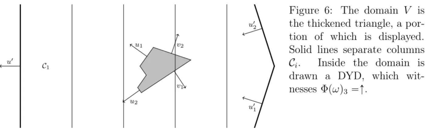
In this section we define our main tool – the droplet algorithm. It can be seen as a significant improvement on the α-covering and u-iceberg algorithms [7, Definitions 6.6 and 6.22], many of whose techniques we adapt to our setting.
We will work in an infinite domain Λ defined as follows (see Figure 2). Fix some vector a0 P R2 and let
B “Hu1 Y Hu1
1pa0q Y Hu12pa0q,
Λ“R2zB, (6)
where the directions u1, u1
1 and u12 are those defined in Lemma 4.1. In other words, Λ is a
cone with sides perpendicular to u1
1 and u12 cut along a line perpendicular to u1. The reader
is invited to simply think that B is a half-plane directed by u1, which will not change the
reasoning.
5.1
Clusters and crumbs
Let Γ be the graph with vertex set Z2 but with x „ y if and only if }x ´ y} ď C
2. Let Γ1 be
defined similarly with C2 replaced by C21. Given a finite K Ă Λ X Z2, we say that κĂ K is a
connected component of K in Γ if the subgraph of Γ induced by the vertex set κ is connected and there do not exist vertices xP Kzκ and y P κ such that x „ y in Γ.
a0 B Λ u1 u11 u1 2
Figure 2: The open domain B defined in (6) is shaded, while its complement Λ is not. The lines are the boundaries of the three half-planes defining B. Note that if a0 R Hu1, then Λ becomes simply a cone.
Crumbs For a given finite set K Ă Λ X Z2 of infections we would like to have a notion of a
connected component being ‘big’ or ‘small’. ‘Small’ components will be dubbed ‘crumbs’ and will play a negligible perturbative role in the bootstrap percolation process, by inducing only ‘very localised’ growth and being ‘well isolated’ from the rest of the infections. A sufficient condition for this, as identified in [7], is that |κ| ă α. However, contrary to what was the case in [7], we need the notion of ‘crumb’ to be stable under the closure (with respect to the bootstrap percolation process), i.e. the closure of a ‘crumb’ to still be a ‘crumb’. We thus identify as ‘crumb’ any component, which is the closure of a set of size less than α. Also taking into account the boundary, this leads us to the following notion.
Definition 5.1 (Crumb). Fix a finite set K Ă Λ X Z2 and let κ be a connected component
of K in Γ. We say that κ is a crumb for K if the following conditions hold. • For all xP κ we have dpx, Bq ą C2.
• There exists a set Pκ Ă Z2 such that rPκs Ą κ and |Pκ| “ α ´ 1.
First properties of crumbs It follows from the definition that a crumb κ for K is at distance more than C2 fromB Y pKzκq. Moreover, the closure of a crumb is within bounded
distance from the crumb, as we shall see in Corollary 5.17 (see Figure 5a). Also, crumbs have diameters much smaller than C3, as we shall see in Corollary 5.17. The proofs of this
corollary and Observation 5.16, which it follows from, are both independent of the rest of the argument and are only postponed for convenience. Nevertheless, we allow ourselves to use these (easy) results ahead of their proofs.
These properties justify and quantify the intuition that crumbs are ‘small’, that they only grow ‘locally’, and it is clear that (if we disregard the boundary) the closure of a crumb is a crumb.
Modified crumbs Unfortunately, if K is the union of two crumbs at distance slightly larger than C2, it is not necessarily true that rKs is still composed of crumbs (recall that, albeit
locally, crumbs can grow under the bootstrap percolation process), which can be disastrous. This is the reason for introducing ‘modified crumbs’ with C1
2 ! C2, so that in the scenario
above all connected components ofrKs in Γ1 are ‘modified crumbs’ (there may now be more
than two of them).
Definition 5.2(Modified crumb). We define a modified crumb by replacing in Definition 5.1 Γby Γ1 and C
In the sequel we will encounter more ‘modified’ notions and constants (like C1
2). These will
be applied to K equal to the closure rK1sB of some K1, which is our initial set of infections.
Our ultimate goal is to ensure that simply using these modified notions based on (much smaller) modified constants will compensate the closure operation.
Clusters We next consider connected components which are not crumbs. Since they can be very large (particularly so if we are working with the closure of a set), we cut them up into (possibly overlapping) pieces termed ‘clusters’, which have bounded size. Roughly speaking, a ‘cluster’ is any ‘big, but not too big’ connected set of infections.
Definition 5.3 (Cluster). Fix a finite set K Ă Λ X Z2. Let κ be a connected component of
K in Γ which is not a crumb. We say that a subset C of κ is a cluster for K if the following conditions hold.
• diampCq ď C3.
• C is connected in Γ (i.e. C is a connected component of C in Γ).
• Either C “ κ or for all x P κzC and y P C such that x „ y in Γ we have diampC Ytxuq ą C3.
A cluster is called boundary cluster if it is at distance at most C2 from B. For a cluster C
we denote by QpCq the smallest open quadrilateral with sides perpendicular to S containing the settx P R2: dpx, Cq ă C
4u.
We similarly define modified cluster and modified boundary cluster by replacing Γ by Γ1
and C2 by C21. For a cluster or modified cluster C we denote by Q1pCq the smallest open
quadrilateral with sides perpendicular to S containing the settx P R2: dpx, Cq ă C1 4u.
Identifying clusters and crumbs In order to identify the clusters and crumbs of K, one may proceed as follows. Determine the connected components of K in Γ and consider each of them separately. For a given component κ first check if it is at distance at most C2 from
B. If so, then it is not a crumb and will give rise to clusters. If not, then check if κ is the closure of at most α´ 1 sites. If this second verification succeeds, then κ is determined to be a crumb and, as mentioned above, it must have diameter much smaller than C3.
If κ is thus determined not to be a crumb, we proceed to identify its clusters. If diampκq ď C3, then there is a single cluster — κ — and we are done. If not, we construct the clusters
of κ by the following algorithm. Initialise the set C “ ∅. If there exists y P κzC such that C Y tyu is connected in Γ and has diameter at most C3, then replace C by C Y tyu and
repeat. If several such y exist, then we do this for each possible y in parallel. The clusters containing x are all possible sets C obtained via this algorithm to which no y can be added. In particular, this provides us with a partition of K into well separated crumbs, single clusters equal to their corresponding connected component and sets of overlapping clusters whose union is a connected component of diameter larger than C3.
First properties of clusters Following the algorithm above, we obtain some basic prop-erties of clusters.
Observation 5.4. Let C be a non-boundary cluster or non-boundary modified cluster for a finite K Ă Λ X Z2. Then |C| ě α.
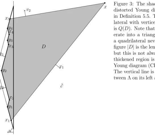
x1 x2 x3 x4 x5 x y2 y1 y3 y4 y v2 v1 u1 u2 u1 D B
Figure 3: The shaded region D is a distorted Young diagram (DYD) as in Definition 5.5. The larger quadri-lateral with vertices x, x1, y and x5
is QpDq. Note that QpDq can degen-erate into a triangle, but we call it a quadrilateral nevertheless. On the figure|D| is the length of the v1 side,
but this is not always the case. The thickened region is the cut distorted Young diagram (CDYD) CpDq of D. The vertical line is the boundary be-tween Λ on its left andB on its right.
Proof. Let κ be the connected component of K in Γ containing C. If diampκq ď C3, then
C“ κ and κ would be a crumb if we had |κ| ď α ´ 1, by taking Pκ Ą κ. If, on the contrary,
diampκq ą C3, then diampCq ě C3´ C2 (by the third condition of Definition 5.3) and we can
choose C3 large enough to have C3C´C2 2 ě α.
Finally, for every cluster C we have diampCq ď C3, so C intersects at most 25C
2 3 other
clusters. Also, QpCq Ą rCs, since QpCq X Z2 Ą C is stable. Furthermore, diampQpCqq “
ΘpC4q, as diampCq ď C3. Analogous statements hold for modified clusters.
5.2
Distorted Young diagrams
We now define the shape that our ‘droplets’ will have, which resembles Young diagrams5
. The following definitions are illustrated in Figure 3.
Definition 5.5 (DYD). A distorted Young diagram (DYD) is a subset of R2 of the form
pHv1pxq X Hv2pxqq X
č
iPI
pHu1pxiq Y Hu2pxiqq (7)
for a finite set I, some set X “ txi: iP Iu of vectors xi P R2 and xP R2. The vectors xi and
x are uniquely defined up to redundancy (and up to the convention that all xi are on the
topological boundary of the DYD). Alternatively, a DYD can also be defined by pHv1pxq X Hv2pxqq X
ď
iPI
pHu1pyiq X Hu2pyiqq, (8)
5
For the 3-rule model alluded to in Section 3 stable sets consist precisely of Young diagrams and the directions S provided by Lemma 4.1 can be arbitrarily close to the four axis directions, yielding Young diagrams.
where yi are the convex corners of the diagram rather than the concave ones.
For any DYD D we denote by y the vector such that xy, ujy “ sup
aPD
xa, ujy “ max
iPI xyi, ujy
for j P t1, 2u. We further denote
QpDq “ Hu1pyq X Hu2pyq X Hv1pxq X Hv2pxq,
i.e. the minimal open quadrilateral containing D with sides directed by S. In these terms, for any cluster or modified cluster C we have that QpCq and Q1pCq are DYD, QpQpCqq “ QpCq
and QpQ1pCqq “ Q1pCq.
Definition 5.6 (CDYD). A cut distorted Young diagram (CDYD) is a subset of R2 of the
form
ΛX pHu1pyq X Hu2pyqq X
č
iPI
pHu1pxiq Y Hu2pxiqq
for a finite set I and some vectors xi P R2 and y P Λ. Alternatively, one can write
ΛXď
iPI
pHu1pyiq X Hu2pyiqq,
where yi P Λ are the convex corners.
For a DYD, D, we denote by CpDq the CDYD defined by the same xi and y or the same
yi. We extend the notation CpDq to CDYD by setting CpDq “ D if D is a CDYD. Note
that by Lemma 4.1 all DYD and CDYD are stable for the bootstrap percolation dynamics (restricted to Λ). Also pay attention to the fact that CDYD are not necessarily connected, contrary to DYD.
Definition 5.7 (Size). For a DYD D we set πpDq “ tx P R: D y P D, xy, v1` π{2y “ xu to
be its projection (parallel to v1) and|D| “ sup πpDq ´ inf πpDq to be its size – the length of
the projection. For a CDYD D we denote its size diampDq{C1 by |D|.
Note that if D is a DYD, then |D| “ |QpDq| by Lemma 4.1 and the assumption we made that u2 ă v1 ´ π{2. Furthermore, for all DYD diampDq “ Θp|D|q again by Lemma 4.1
with constants depending only on S. One should be careful with the meaning of size for disconnected CDYD, but it will not cause problems, as all CDYD arising in our forthcoming algorithm are connected.
Observation 5.8. Note that for any dě 1 the number of discretised DYD and CDYD (i.e. intersections of a DYD or CDYD with Z2) containing a fixed point a P R2 of diameter at
most d is less than cd for some constant c depending only on S.
Proof. Note that a DYD or CDYD is uniquely determined by its rugged edge formed by its u1 and u2-sides. However, this edge injectively defines an oriented percolation path with
directions perpendicular to u1 and u2 on the lattice
tx P R2: Dx
1, x2 P Z2,xx, u1y “ xx1, u1y, xx, u2y “ xx2, u2yu
(except its endpoints, which lie on similar lattices). Since the graph-length of this path is bounded by Opdq and its endpoints are within distance d from a, the result follows.
x11 x12 x13 x14 “ x8 y11 y12“ y3 y1 3 “ y5 y1 4“ y7 y1 x1 y24“ y6 y2 3 “ y4 y2 2 “ y2 y21 “ y1 x2 4 x2 3 x2 2“ x2 x21“ x1 y2 x2 x y x7 x6 x5 x4 x3 D1 D2 D1_ D2
Figure 4: The shaded region D1and thickened region D2are DYD. Their respective
quadrilat-erals QpDiq are completed by dashed lines. Their span D1_D2is hatched and its quadrilateral
QpD1_ D2q is also completed by dashed lines.
5.3
Span
We next introduce a procedure of merging DYD and CDYD. This will be used only for couples of intersecting ones, but can be defined regardless of whether they intersect. The operation is illustrated in Figure 4.
Lemma 5.9. For any two DYD, D1 and D2, the minimal DYD containing D1Y D2 is well
defined. We denote it by D1_ D2 and call it their span. The operation _ is associative 6
and commutative.
Proof. Let D1be defined by Y1 “ tyi1: iP Iu, x1 (see (8)) and similarly for D2. Let xP R2 be
the vector such that Hvipx
1qYH vipx
2q “ H
vipxq for i P t1, 2u. Let Y be the set of yi P Y
1YY2
such that for all yj P Y1 Y Y2 with yi ‰ yj we have Hu1pyjq X Hu2pyjq Č Hu1pyiq X Hu2pyiq.
We denote by D the DYD defined by Y, x and claim that for any DYD D1 Ą D
1YD2 we have
D1 Ą D, which is enough to conclude that D “ D
1 _ D2 is well defined. Let D1 be defined
by Y1, x1.
6
Note that for each yi P Y (and in fact in Y1 Y Y2) there is a sequence of points in
D1 or D2 converging to yi, so that (by extraction of a subsequence) there exists yj1 with
Hu1py
1
jq X Hu2py
1
jq Ą Hu1pyiq X Hu2pyiq. Similarly, there is a sequence of points in D1 or D2
converging to the boundary of Hv1pxq, so that Hv1px
1q Ą H
v1pxq and similarly for v2. Thus,
we do have D1 Ą D.
Finally, the commutativity is obvious and the associativity follows from the characterisa-tion of D1_ D2 as the minimal DYD containing both D1 and D2.
We analogously define the span D1_ D2 of two CDYD D1 and D2 – the minimal CDYD
containing both – and note that it coincides with their union (which is also commutative and associative). We also define the span C_ D of a DYD D and a CDYD C as the minimal CDYD containing pC Y DqzB, which coincides with C _ CpDq. The proof that it is well defined is analogous to Lemma 5.9.
We have thus defined an associative and commutative binary operation _ on all DYD and CDYD. Moreover, the idempotent unary operation Cp¨q is distributive with respect to _ and CpD1q _ D2 “ CpD1 _ D2q. Furthermore, the span of several DYD is the minimal
DYD containing all of them, while the span of several DYD and at least one CDYD is the minimal CDYD containing all the corresponding CDYD.
5.4
Droplet algorithm and spanned droplets
A droplet is any DYD contained in Λ or CDYD. We are now ready to define our droplet algorithm, which takes as input a finite set K Ă Λ X Z2 of infections and outputs a set D of
disjoint connected droplets. It proceeds as follows.
• Form an initial collection of DYD D consisting of QpCq for all clusters C of K. If a DYD DP D intersects B, replace it by its CDYD, CpDq, to obtain a droplet.
• As long as it is possible, replace two intersecting droplets of D by their span. If the span intersectsB, replace it by its CDYD to obtain a droplet.
• Output the collection D obtained when all droplets are disjoint.
We similarly define the modified droplet algorithm by replacing QpCq by Q1pCq and clusters
by modified clusters above.
The output D is clearly a collection of disjoint connected droplets. Indeed, by induction all xi corners of droplets remain in Λ (see Figure 4), so that DYD remain connected when
replaced by CDYD.
Remark 5.10. From the results of Section 5.3 it is clear that the order of merging does not impact the output of the algorithm, which is thus well defined. It can also be expressed as the minimal collection of disjoint droplets containing the intersection with Λ of the original collection of quadrilaterals. This minimal collection is well defined. Consequently, the union of the output is increasing in the input.
Definition 5.11 (Spanned droplets). Let D be a droplet and K Ă Z2. We say that D is
spanned for K with boundaryB if the output of the droplet algorithm for K XD has a droplet containing D. We omit K andB if they are clear from the context. Similarly, D is modified spanned if the output of the modified droplet algorithm for KX D has a droplet containing D.
Note that, when seen as an event, a droplet being spanned is monotone. It is also clear that each droplet appearing in (the intermediate or final stages of) the droplet algorithm is spanned and similarly for the modified droplet algorithm. Indeed, the clusters responsible for creating a droplet in the course of the algorithm are contained in the droplet, so each of them is still a cluster of KX D (recall that crumbs have diameter much smaller than C3).
5.5
Properties of the algorithm
We next establish several properties of the algorithm. The approach is similar to the one of [7] with the notable exception of the key Closure Proposition 5.20. We start with the following purely geometric statement.
Lemma 5.12(Subadditivity). Let D1 and D2 be two DYD or CDYD with non-empty
inter-section. Then
|D1_ D2| ď |D1| ` |D2|.
Furthermore, if D is a DYD intersectingB, then |CpDq| ď |D|.
Proof. First assume that D1 and D2 are DYD. Since |D| “ |QpDq| for any DYD D and
D1 _ D2 Ă QpQpD1q _ QpD2qq, it suffices to prove the assertion for merging quadrilaterals
instead of DYD. But in that case it is not hard to check directly and is a particular case of Lemma 15 of the first arXiv version of [8] (or Lemma 23 of the second version). Since similar (but actually slightly more involved) details were omitted in the proof of the corresponding Lemma 4.6 of [8] and differed to earlier versions, we will not go into useless detail here either. To give a sketch of a possible argument, one can check that for fixed shapes of QpD1q and
QpD2q the maximal QpQpD1q _ QpD2qq is achieved when their intersection is reduced to a
vertex. Yet, in those configurations one can obtain the v1 and v2 sides of QpQpD1q _ QpD2qq
as the union of those of QpD1q and translates of those of QpD2q (see Figure 4). This concludes
the proof, as only v1 and (possibly) v2 sides contribute to | ¨ | by Lemma 4.1.
Next assume that D1 is a DYD and D2 is a CDYD. Let Y “ tyi: i P Iu be the set of
vectors defining CpD1q and let a P D1XD2. Since Y Ă D1, we have that dpyi, aq ď diampD1q.
It then easily follows that the CDYD defined by only one corner, yi, which we denote Cpyiq,
is within distance OpdiampD1qq from Cpaq. But then CpD1q “ ŤiPICpyiq is within distance
OpdiampD1qq from Cpaq. Thus, |D1_ D2| ď pdiampD2q ` OpdiampD1qqq{C1 ď |D2| ` |D1|,
since diampD1q “ Op|D1|q and all implicit constants depend only on S and are thus much
smaller than C1.
Next assume that D1 and D2 are CDYD. Then the statement is trivial, because D1_D2 “
D1Y D2, so diampD1q ` diampD2q ě diampD1_ D2q by the triangle inequality.
Finally, let D be a DYD intersecting B. Then, |CpQpDqq| ě |CpDq| and |QpDq| “ |D|, so we may assume that D “ QpDq and prove |CpDq| ď |D|. But in this case it is easy to see that diampCpDqq “ OpdiampDqq “ Op|D|q with constants depending only on S, which concludes the proof.
The subadditivity lemma will be used to prove the next two adaptations of classical results.
Lemma 5.13 (Aizenman-Lebowitz). Let K be a finite set and let D be a spanned droplet with |D| ě C2
4. Then for all C42{C1 ď k ď |D|{C1 there exists a connected spanned droplet
Proof. By Lemma 5.12 at each step of the droplet algorithm the largest size of a droplet appearing in the collection at most doubles. Initially the largest size is at most C1C4 and in
the end there is a (unique) droplet D2 Ą D, so that |D2| ě |D|{C
1 ě C42{C1 ą C1C4. Then
there is a stage of the algorithm at which the maximal size of a droplet in D is between k and 2k, which is enough since all droplets appearing in the droplet algorithm are connected and spanned. The proof for modified spanned droplets is identical, using the modified droplet algorithm.
Lemma 5.14(Extremal). Let K Ă Z2 and let D be a droplet spanned for K. Then the total
number of disjoint clusters for KX D in D is at least diampDq{C2 4.
Proof. In this proof all clusters will be clusters for KX D. Assume that at the initial stage of the algorithm there are k clusters (not disjoint). One can then find k{C1
4 disjoint ones, since
their diameter is at most C3. Furthermore, by Lemma 5.12 the total size of droplets in the
collection D is decreasing, so that|D|{C1 ď |D1| ď kC1C4, where D1 Ą D is some droplet in
the output of the algorithm. Indeed, |QpCq| ď C1C4 for all clusters C. This concludes the
proof, since|D| ě diampDq{C1 for all DYD and CDYD.
We next transform this extremal bound into an exponential decay of the probability that a droplet is spanned until saturation at the critical size. In the following lemma, we identify the configuration ω having law µ and the set of its zeroes.
Lemma 5.15 (Exponential decay). Let D be a droplet with |D| ď 2{pC5qαq. Then
µpD is spanned for ωq ă expp´C4|D|q.
Proof. Let D be a droplet with |D| ď 2{pC5qαq, so that diampDq “ d ď 2C1{pC5qαq. By
Lemma 5.14 if D is spanned for ω, it contains at least d{C2
4 disjoint clusters for ω X D,
each one having diameter at most C3. Each non-boundary cluster has at least α sites by
Observation 5.4, while boundary clusters are non-empty and located at distance at most C2
fromB. Thus, we have the union bound µpD is spanned for ωq ď d{C2 4 ÿ l“0 ˆC2α 3 d2 l ˙ˆ C3d d{C2 4 ´ l ˙ qlα`pd{C42´lq ď d{C2 4 ÿ l“d{p2C2 4q pC1 4qαd2{lql.ed` d{C2 4 ÿ l1“d{p2C2 4q pC1 4qd{l1ql 1 .ed ď d{C2 4 ÿ l“d{p2C2 4q ˜ C1 4e2C 2 4qα 1{p2C2 4q ¨ 2C1 C5qα ¸l ` d{C2 4 ÿ l1“d{p2C2 4q ´ 2C42C41e 2C2 4q ¯l1 ď expp´C4dq,
recalling that C5 is sufficiently large depending on C4, C41 and C1.
Our next aim is to prove that the closure of a set is contained in its droplet collection up to very local infections next to initial ones. To that end we will need some preliminary results, similar to those used by Bollobás, Duminil-Copin, Morris and Smith [7].
Observation 5.16(Lemma 6.5 of [7]). Let u be a rational non-semi-isolated stable direction. Let K Ă Z2 with |K| ă αpuq (if αpuq “ 8 the condition is that K is finite, but there is no
a priori bound on its size). Then there exists a constant CpU, u, |K|q not depending on K such thatrKsHu is within distance CpU, u, |K|q from K.
Since we will require some improvements later, we spell out a proof of the above result for completeness (actually our proof is slightly different from the one in [7]).
Proof of Observation 5.16. We prove the statement by induction on|K|. For a K “ txu this is easy, since ifxx, uy is sufficiently large rKsHu “ K and otherwise there is a single possible
configuration for each value ofxx, uy up to translation. Assume the result holds for |K| ă n. If one can write K “ K1\ K2 with K1, K2 ‰ ∅ and dpK1, K2q ą 2CpU, u, n ´ 1q ` Op1q, then
rKsHu “ rK1sHu\ rK2sHu, since rK1sHu and rK2sHu are at sufficiently large distance, hence
no site can use both to become infected. Assume that, on the contrary, there are no large gaps between parts of K. There is a finite number of such K up to translation and for each of these rKs is finite (e.g. since K is contained in a quadrilateral with sides perpendicular to S), so within uniformly bounded distance from K. Therefore, if Hu is sufficiently far
from K, rKsHu “ rKs. Otherwise, there is a finite number of possible K up to translation
perpendicular to u and for each of them rKsHu is finite, so that one can indeed find a finite
uniform constant CpU, u, nq as claimed.
A quantitative version of this result was proved by Mezei and the first author [21]. An easy corollary of Observation 5.16 is the fact that crumbs can only grow very locally (see Figure 5a).
Corollary 5.17. Let C1 be sufficiently large depending on U. Let K Ă Z2 with |K| ă α.
Then rKs is within distance C1{p6αq from K. Also, for a (modified) crumb κ we have that
diamprκsq ď αC2 and rκs is within distance C1 from κ.
Proof. The first assertion follows from Observation 5.16, since if it were wrong, one could simply translate a set K sufficiently far from a half-plane yielding a contradiction with the observation.
Next consider a (modified) crumb κ and Pκ minimal with |Pκ| ă α and rPκs Ą κ. Then
rκs Ă rPκs is within distance C1{p6αq from Pκ. If the sites of Pκ are not connected in the
graph Γ2 on Z2 with connections at distance at most C
1` C2, then either κ is not connected
in Γ or Pκ is not minimal, which are both contradictions. Similarly, if there is no site of κ at
distance smaller than C1{p2αq from a C1{p2αq-connected component of Pκ, that component
can be removed from Pκ, contradicting minimality. Hence, Pκ is within distance C1{2 from
κ. The result is then immediate, as rκs is within distance C1{2 ` C1{p6αq from κ and its
diameter is at most C1{p3αq ` diampPκq, while diampPκq ď pα ´ 1qpC1` C2q.
In order to treat infection at the concave corners of droplets we will need the following modification of Observation 5.16.
Corollary 5.18. Let u1 and u2 be rational strongly stable directions such that Hu1 Y Hu2 is
stable for the bootstrap percolation dynamics i.e. EU P U, U Ă Hu1 Y Hu2. Let K Ă Z
2 with
|K| ď α ´ 1. Then rKsHu1YHu2 is within distance CpU, u1, u2q from K.
Proof. We apply a similar induction to the one in the proof of Observation 5.16. The only difference is that we can no longer use translation invariance. If dpK, Hu2q ą CpU, u1,|K|q `
Op1q, by Observation 5.16, we have rKsHu1YHu2 “ rKsHu1 and similarly for u1 and u2
inter-changed. We can thus assume that K is within distance C1pU, u
1, u2q from the origin. But
then rK Y Hu1 Y Hu2s Ă Hu1 Y Hu2 Y Hu1pC
2pU, u
1, u2qu1q, where u1 “ pu1` u2q{2, since the
latter region is stable by the hypothesis on u1, u2.
We next transform these results for infinite regions into a result for droplets. It states that a crumb next to a droplet cannot grow significantly (see Figure 5b).
C1
ď C2
(a) The dots represent the sites of a crumb. The (discon-nected) circled shape bounds its closure. Note that crumbs may have gaps of size C2while
the growth allowed is only C1! C2. 8 y1 8 y2 8 x x y1 y2 C4u0{C1 C4v0{C1 2C3 8 D D
(b) The shaded region is the shrunken DYD 8Dof the largest DYD D. The solid circles represent crumbs and the dashed arcs are the bound for their growth provided by Lemma 5.19. The modified clusters of the closure are included in the dotted DYD.
Figure 5: Illustrations of Corollary 5.17, Lemma 5.19 and Proposition 5.20.
Lemma 5.19. Let C1 be sufficiently large depending on U and S. Let D be a DYD at distance
at least C3 fromB or be a CDYD and let κ be a crumb. Then rκsDYB “ rκsD is within distance
C1 of κ.
Proof. Assume that D is a DYD at distance at least C3 fromB. The proof of [7, Lemma 6.10]
applies using (7), Observation 5.16, Corollary 5.18 and the arguments in the proof of Corollary 5.17 to give the result for rκsD, which is therefore at distance at least C2´ C1 from B since
dpκ, Bq ě C2, so that in fact rκsD “ rκsDYB.
Assume next that D is a CDYD. Then actually DY B can be viewed as a DYD on the entire plane without boundary specified by an infinite number of vectors xi, so that we are
in the previous case. In order to avoid introducing the corresponding notion of infinite DYD, one can consider an increasing exhaustive sequence of DYD Di converging to DY B in the
product topology and apply the previous result forrκsDi, which will thereby apply to DY B.
Finally, rκsD “ rκsDYB follows, since dprκsDYB,Bq ě C2´ C1.
The next proposition is key to making the output of the algorithm essentially invariant under the KCM dynamics without having to pay for the fact that the closure for the bootstrap percolation dynamics of infections at equilibrium is not at all at equilibrium itself. The proof is illustrated in Figure 5b.
Proposition 5.20 (Closure). Let K be a finite set and D1 be the collection of droplets given
by the modified droplet algorithm with inputrKsB. Let D be the output of the droplet algorithm
for K. Then
Proof. Let K be the set of crumbs for K. Set κ0 “ ŤκPKκ.
Claim 1. For each crumb κ P K its closure rκs “ rκsB consists of at most α´ 1 modified
crumbs of rκs all contained within distance C1 from κ.
Proof of Claim 1. There exists a set Pκ as in Definition 5.1, such that rPκs Ą κ and thus
rPκs Ą rκs, which proves that all connected components of rκs for Γ1 are modified crumbs.
The fact that rκs is within distance C1 of κ (and thus at distance at least C21 from B) was
proved in Corollary 5.17, which also shows that rκs “ rκsB, since κ is at distance more than
C2 from B.
We can thus define K1pκq to be the set of modified crumbs of rκs
B, so that their union
is disjoint and equal to rκsB. Moreover, crumbs in K are at distance at least C2 from each
other, so for any two of them κ1 ‰ κ2 we have that any κ11 P K1pκ1q and κ12 P K1pκ2q are at
distance at least C2´ 2C1 " C21 and also at such distance from B, so that rκ0sB “ ŤκPKrκsB
has no modified cluster and consists of modified crumbs at distance at most C1 from κ0.
For a droplet D P D consider the set of vectors Y and x (x is absent for CDYD) defining it. Then define 8Y “ Y ` C4u0{C1 and 8x “ x ` C4v0{C1, where u0 P R2 is the vector such
that xu0, u1y “ xu0, u2y “ ´1 and v0 is defined identically in terms of v1 and v2. We denote
by 8D the droplet defined by 8Y and 8x and call it a shrunken droplet. Let D0 “ ŤDPDD and
8
D0 “ ŤDPDD. It is clear that 88 D is at distance at least C4{C1 from ΛzD for all droplets
D. In particular, all shrunken droplets are at distance at least C4{C1 from each other and
shrunken DYD are at distance at least C4{C1 from B, so that Lemma 5.19 applies to them
and r 8D0sB “ 8D0.
Claim 2. 8D0Y κ0 Ą K.
Proof of Claim 2. Note that it is enough to prove that the clusters of K are contained in 8D0.
Assume that there exists aP Kz 8D0 and aP C for some cluster. Then, QpCq X Λ is contained
in some D P D, which is defined by Y and x (x is absent for CDYD). Then since a R 8D, either for all 8yi P 8Y we have aR Hu1p 8yiq X Hu2p 8yiq or a R Hv1p8xq X Hv2p8xq. In the former case,
a´ C4u0{C1 R Hu1pyiq X Hu2pyiq for all yi P Y . However, QpCq contains the ball of radius C4
centered at a and }u0} “ Op1q, so we get a contradiction. If a R Hv1p8xq X Hv2p8xq, the first
point on the segment from a to a´ C4v0{C1 that is not in D is in Λ and in QpCq, hence a
contradiction.
Claim 3. The set rKsBzrκ0sB is within distance C3 of 8D0.
Proof of Claim 3. By Claim 2 we have K0 “ 8D0 Y κ0 Ą K. It then clearly suffices to prove
that rK0sBzrκ0sB is within distance C3 of 8D0.
Consider a crumb κP K at distance at most C2 from 8D0, so at distance at most C2 from
a shrunken droplet 8D and necessarily at distance at least C4{C1 ´ C2´ C3 from any other
shrunken droplet and fromB if D is a DYD. By Lemma 5.19 rκsD8 “ rκsDYB8 is within distance
C1 of κ. Hence,
rK0Y Bs “ 8D0Y B Y rκ0s Y
ď
κ,D
rκsD8, (9)
where the last union is on couplespκ, Dq as above. Indeed, all rκsD8 and rκs (for different κ)
are at distance at least C2´ 2C1 from each other and from 8D0z 8D (by the reasoning above),