(will be inserted by the editor)
Flow-Aware Workload Migration in Data Centers
Yoann Desmouceaux · Sonia Toubaline · Thomas Clausen
Abstract In data centers, subject to workloads with heterogeneous (and sometimes short) lifetimes, workload migration is a way of attaining a more efficient utilization of the underlying physical machines. To not introduce per-formance degradation, such workload migration must take into account not only machine resources, and per-task resource requirements, but also applica-tion dependencies in terms of network communicaapplica-tion.
This paper presents a workload migration model capturing all of these constraints. A linear programming framework is developed allowing accurate representation of per-task resources requirements and inter-task network de-mands. Using this, a multi-objective problem is formulated to compute a re-allocation of tasks that (i) maximizes the total inter-task throughput, while (ii) minimizing the cost incurred by migration and (iii) allocating the maximum number of new tasks.
A baseline algorithm, solving this multi-objective problem using the ε-constraint method is proposed, in order to generate the set of Pareto-optimal solutions. As this algorithm is compute-intensive for large topologies, a heuris-tic, which computes an approximation of the Pareto front, is then developed, and evaluated on different topologies and with different machine load factors. These evaluations show that the heuristic can provide close-to-optimal solu-tions, while reducing the solving time by one to two order of magnitudes.
Yoann Desmouceaux∗†, E-mail: [email protected], +33158045314 (corresponding author)
Sonia Toubaline‡, E-mail: [email protected], +33144054415 Thomas Clausen∗, E-mail: [email protected], +33169334088 ∗École Polytechnique, 91128 Palaiseau, France
†Cisco Systems Paris Innovation and Research Laboratory (PIRL), 92782 Issy-les-Moulineaux, France
‡Université Paris-Dauphine, PSL Research University, CNRS, LAMSADE, 75016 Paris, France
Neither the entire paper nor any part of its content has been published or has been accepted for publication elsewhere. It has not been submitted to any other journal.
Keywords
Data Center Networking, VM Migration, Application-Aware Allocation, MILP, Multi-objective Optimization, Pareto Optimality.
1 Introduction
1.1 Context and Approach
Virtual Machine (VM) live migration [1] is a way to transfer a VM from a host to another, by iteratively copying its memory. It is further suggested in [2,3] that it is possible to perform live migration of individual processes or containers, thus attaining one further level of granularity of task placement flexibility. In virtualized data centers, applications thus need not be tied to a specific machine – and their relocation can become part of a “natural” mode of data center operation. This provides a way to accommodate hardware failures without service downtime, of course, but more generally may be beneficial to the efficiency of the whole data center in terms of resource usage and execution efficiency.
With the desirability of task (VM or container, also occasionally called “workload” in literature [4]) mobility established, the question of an optimal task migration mechanism naturally arises, which will be investigated in this paper. Task placement has been studied, and current approaches provide mathematical models focusing on optimal usage of resources and on flow min-imization [5], or models that also consider migration but do not take detailed the network topology into account [6,7].
This paper introduces a multi-objective linear programming model of task migration that satisfies per-node resources constraints and inter-nodes com-munication requirements while minimizing the cost incurred by migrations. The fundamental assumptions are (i) that tasks have inter-communication de-mands that change with time, (ii) that tasks that communicate benefit from be-ing topologically close, and therefore (iii) that changes in inter-communication demands may make a current task placement suboptimal, suggesting possible efficiency gains by relocation. Hence, the developed multi-objective linear pro-gramming model of task migration is intended to run iteratively, at regular time intervals. It uses task inter-communication demands to decide if and where to reallocate tasks so as to provide the best possible task placement, while minimizing a migration cost. Network constraints are taken into account by modeling the traffic as a multi-commodity flow problem, where a commod-ity represents an inter-task communication demand.
1.2 Related Work
Data center traffic has been extensively studied: it has been shown that the amount of intra-rack traffic is as voluminous as is extra-rack traffic [8], and that
patterns emerge when considering the traffic matrix between interdependent tasks [9,10]. Some task pairs communicate more than others, in which case it makes sense to locate those on either the same machine, or on machines close to each other in the network topology. Therefore, data center architectures have been studied which take communication dependencies between workloads into account, from a network systems perspective [11, 12]. This motivates the need for models that can place workloads according to their pairwise communication demands.
The VM placement problem consists of finding an efficient assignment of VMs to machines within a data center, satisfying a set of constraints (re-sources, possibly traffic demand) with respect to one or more objective func-tions such as energy consumption minimization [4,13,14,15,16], communica-tion cost minimizacommunica-tion [17, 5], network traffic minimizacommunica-tion or resource utiliza-tion maximizautiliza-tion. Different optimizautiliza-tion approaches have been proposed for the VM placement problem: solution techniques include deterministic algo-rithms, heuristics, meta-heuristics and approximation algorithms. Surveys of these methods can be found in [18, 19,20,21]. Many approaches have been pro-posed that aim at optimizing a single objective. Multi-objectives formulations have also been introduced, but they are often reduced to a mono-objective problem, failing to provide a set of Pareto-optimal solutions.
Single-objective approaches: In [6], a model that considers resources constraints as well as dependencies between applications is proposed, which then re-allocates VMs while minimizing the migration impact. Contrary to the approach presented in this paper, [6] does not consider changing com-munication demands between applications, but only migrate VMs located on overloaded machines. In [7], this model is refined by incorporating finer-grained server-side constraints, as well as network capacities of the machines. In [22], the problem of optimizing both VM placement and traffic flow routing so as to save energy is considered. A model is formulated that minimizes the power consumption of switches and links, while satisfying capacity and traffic de-mands constraints. In [17], a network-aware model is considered that places VMs with the aim of minimizing communication cost. A greedy consolidation algorithm is proposed, consisting of identifying VM clusters based on network traffic (using a cost matrix). In [10], a traffic-aware VM placement model is introduced, where the objective is to minimize the aggregate traffic rates per-ceived by every switch. A two-tier approach given by a cluster-and-cut heuristic is proposed.
Multi-objective reduced to single-objective: Some VM placement problems are formulated as multi-objectives models, which are then reduced to single-objective models. In [23], the authors consider the placement of VMs on machines by minimizing the size of clusters of VM serving the same jobs, and minimizing the maximum traffic on uplinks of top-of-rack switches. An iterative least-loaded-first based placement algorithm is proposed, which first gives the priority to locality, and then to bandwidth occupancy. In [24], a power-efficient VM placement and migration model is introduced, aiming at minimizing the number of machines used, the network energy consumption
and the network end-to-end delay. The model is solved using a weighted sum approach. In [25], VM placement is considered under three objectives, to be minimized: total resource “waste”, power consumption, and thermal dissipation costs. The solution approach is a combination of a generic grouping algorithm and a fuzz multi-objective evaluation. In [26], a VM management framework considering initial VM placement and VM migration is introduced, with three objectives: elimination of thermal hotspots, minimization of power consump-tion and applicaconsump-tion performance satisfacconsump-tion. The problem is solved using a weighted sum approach.
Pure multi-objective approaches: In [27], a bi-objective mathemati-cal formulation for VM placement is proposed, aiming at minimizing resource wastage and power consumption. A multi-objective ant colony system algo-rithm is proposed to generate the set of non dominated solutions. In [28] (extending [29]), a multi-objective formulation of the VM placement problem is introduced, aiming at minimizing energy consumption and network traffic, and maximizing economical revenue while satisfying a service level agreement (SLA). A memetic algorithm given by an evolutionary process is proposed, and a Pareto set approximation is returned.
1.3 Problem Restatement
For some distributed computing applications, where tasks frequently commu-nicate with each other, the limiting factor for the completion of a running task is not necessarily its actual location (assuming that the task is allocated with the full physical resources it needs), but can be the throughput at which it exchanges data with other tasks. Furthermore, if those tasks have changing traffic requirements, migrating them within the data center can be an efficient way to re-organize the load across all available machines so as to optimally satisfy these requirements.
With these two assumptions as a baseline – tasks need to be allocated according to their communication requirements, and those requirements can change over time – the multi-objective mathematical problem introduced in this paper consists of determining a task placement which satisfies machine, network and applications constraints, while (i) maximizing the number of new tasks to be assigned, (ii) minimizing the migration cost and (iii) maximizing the total inter-task throughput.
The contribution of this paper is therefore threefold: (i) it formulates a model of workload migration which uses an accurate description of network demands and of the network topology; (ii) it proposes a multi-objective ap-proach which generates the set of Pareto-optimal solutions, from which the operator can choose according to operational tradeoffs; and (iii) it proposes a heuristic method that can generate an approximate Pareto front while greatly reducing solving time as compared to obtaining the exact solution.
Evaluations show that the sets of solutions generated by this approximation method remain close to their optimal counterparts, regardless of the topology and the task-to-machine ratio.
1.4 Paper Outline
The remainder of this paper is organized as follows. Section 2 introduces the framework needed to represent the state of the data center. Section 3 presents the mathematical formulation proposed for the flow-aware workload placement and migration problem, given by a multi-objective Mixed Integer Linear Pro-gram (MILP) [30]. Section 4 describes the algorithm used to generate the set of Pareto-optimal solutions to this problem, and provides a computational ex-ample. An approximation method is proposed in section 5; its performance in terms of solving time and quality of the generated approximate solutions (as compared to the optimal ones) are then evaluated. Finally, section 6 concludes this paper.
2 Data Center Representation
This paper presents a multi-objective time-indexed formulation of a task mi-gration and placement problem. Before detailing the problem formulation (sec-tion 3), resolu(sec-tion (sec(sec-tion 4) and approxima(sec-tion (sec(sec-tion 5), this sec(sec-tion in-troduces the framework used to describe the state (including the topology) of a data center. This is achieved by considering (i) a set of machines, (ii) the network topology connecting them, and (iii) a set of tasks to allocate on these machines. As this model considers workload migration, for which it is necessary to be aware of the evolution of the state of the data center, the model makes the assumption that it is running at a given time t (where t is an abstract index without unit), and that the previous state of the data center corresponds to time (t − 1). Thus as a convention, a variable superscripted with t represents the current state of the data center (to be optimized), and a variable superscripted with (t − 1) is a known input representing the previous state of the data center. A summary of the notations used throughout this paper is provided in Table 1.
2.1 Tasks and Machines
Tasks to be run at time t are represented by a set It. At time t, new tasks
can arrive or existing tasks can finish executing. Arriving tasks correspond to those in It\ It−1. Already existing tasks correspond to those in It∩ It−1, and
among those, the ones that were successfully assigned to a machine at time (t − 1) have priority over new tasks and must be placed to some machine at time t (they can continue execution on the same machine, or be migrated to
Notation Description i, i′, · · · ∈ It Tasks to be run at time t m, m′, · · · ∈ M Machines
s, s′, · · · ∈ S Switches
A ⊆ (M ∪ S)2 Network edges
Amm′ ∈ 2A Path m 7→ m′
cuv> 0 Capacity of link (u, v) κm> 0 Machine CPU capacity
ri> 0 Task CPU requirement
si> 0 Task size
Ct⊆ It× It Communicating tasks at time t dt
ii′> 0 Throughput demand for i 7→ i′at time t xt
im∈ {0, 1} Task i is allocated on machine m at time t ft
ii′(u, v) ∈ R
+ Flow for i 7→ i′along (u, v) at time t Table 1 Inputs and variables to the model
another one, but not be stopped). Terminated tasks correspond to those in It−1\ It, and thus are not of interest to the model.
Machines are represented by a set M . Each machine m ∈ M has a CPU capacity κm > 0 which represents the amount of work it can accommodate.
Conversely, each task i ∈ It has a CPU requirement r
i > 0, representing the
amount of resources it needs in order to run. Finally, each task i ∈ It has a
size1
si > 0. This size will be used to model the cost of migrating the task
from one machine to another.
2.2 Network Model
In order to take application dependencies into account, the physical network topology existing between the machines must be known. To that end, a network is modeled as a directed graph G = (V, A), where V = M ∪ S is the set of vertices, with S the set of switches2
and A the set of arcs. An arc (u, v) ∈ A can exist between two switches or between a machine and a switch, but also between a machine and itself to model a loopback interface (so that two tasks on the same machine can communicate). Each of those arcs represents a link in the network, and has a capacity of cuv> 0. For each ordered pair of machines
(m, m′
) ∈ M2, a list A
mm′ ∈ 2A represents the path from m to m′.
For example, given the topology depicted in Figure 1 with three switches s0, s1, s2and four machines m1, m2, m3, m4, the arcs of the graph will be as
fol-lows: A = {(m1, m1), (m1, s1), (s1, m1), (m2, m2), (m2, s1), (s1, m2), (m3, m3),
(m3, s2), (s2, m3), (m4, m4), (m4, s2), (s2, m4), (s1, s0), (s0, s1), (s2, s0), (s0, s2)}.
The path from e.g., m1 to m3 will be Am1m3 = {(m1, s1), (s1, s0), (s0, s2),
(s2, m3)}.
1For instance, the size of RAM plus storage for a virtual machine.
2This term is used generically to refer to any forwarding node in the network, regardless of its actually being a router or a switch.
m1 m2
s1
m3 m4
s2
s0
Fig. 1 Simple network example
Finally, at a given time t, an ordered pair of tasks (i, i′
) ∈ It× It can
communicate with a throughput demand dtii′ > 0, representing the throughput
at which i would like to send data to i′. Let Gt
d = (It, Ct) be a weighted
directed graph representing these communication demands, where each arc (i, i′) ∈ Ctis weighted by dt
ii′. Gtdwill be referred to as the throughput demand
graph.
3 Mathematical Modeling
Based on the data center framework described in section 2, this section presents a multi-objective Mixed Integer Non Linear Program (MINLP) aiming at op-timizing workload allocation and migration while satisfying inter-application network demands. A linearization as a multi-objective MILP is then derived, allowing for an easier resolution.
3.1 Variables
Two sets of variables are introduced, representing (i) task placement and (ii) the network flow for a particular allocation.
Task placement The aim of the model is to provide a placement of each task i ∈ It on a machine m ∈ M , at a given timestep t. The binary variable xt
im
reflects this allocation: xt
im= 1 if i is placed on m, and xtim= 0 otherwise.
Network flow In order to determine the best throughput that can be achieved between each pair of communicating tasks, a variant of the multi-commodity flow problem [31, p. 58] is used, where a commodity is defined by the existence of (i, i′) ∈ Ct. A commodity thus represents an inter-task communication.
For each link (u, v) ∈ A, ft
ii′(u, v) is a variable representing the throughput
for communication from i to i′
3.2 Constraints
Two sets of constraints are used to model this flow-aware workload migra-tion problem: allocamigra-tion constraints (equamigra-tions (1-3)) represent task allocamigra-tion, whereas flow constraints (equations (4-8)) focus on network flow computation. The allocation constraints represent the relationship between tasks and machines. First, each task i ∈ Itmust be placed on at most one machine:
X
m∈M
xtim≤ 1, ∀i ∈ It (1)
Forcefully terminating a task is not desirable: if a task was running at time t − 1, and is still part of the set of tasks at time t, it must not be forcefully terminated: X m∈M xt−1im ≤ X m∈M xtim, ∀i ∈ It−1∩ It (2)
where xt−1im is a known input given by the state of the system at time t−1. If the task was successfully allocated at time t−1 (i.e. i ∈ It−1andP
m∈Mx
t−1
im = 1)
and is still to be run at time t (i.e. i ∈ It), the left-hand-side of the equation
will be 1, thus forcing allocation of the task at time t.
Finally, the tasks on a machine cannot use more CPU resources than the capacity of that machine:
X
i∈It
rixtim≤ κm, ∀m ∈ M (3)
The flow constraints allow computing the throughput for each commodity (i.e. ordered pair of communicating task). For each link (u, v) ∈ A in the network, the total flow along the link must not exceed its capacity:
X
(i,i′)∈Ct
fiit′(u, v) ≤ cuv, ∀(u, v) ∈ A (4)
For a commodity (i, i′) ∈ Ct, the flow going out of a machine m must not
exceed the throughput demand for the communication from i to i′. Also, the
flow must be zero if task i is not hosted by machine m: X v:(m,v)∈A fiit′(m, v) ≤ d t ii′ x t im, ∀m ∈ M, ∀(i, i ′ ) ∈ Ct (5)
Conversely, for a commodity (i, i′
) ∈ Ct, the flow entering a machine m′
must not exceed the throughput demand for the communication from i to i′
, and must be set to zero if task i′
is not on m′ : X v:(v,m′)∈A fiit′(v, m ′ ) ≤ dtii′ xti′m′, ∀m ′ ∈ M, ∀(i, i′ ) ∈ Ct (6)
Each switch s ∈ S must forward the flow for each commodity – that is, the ingress flow must be equal to the egress flow:
X v:(u,v)∈A ft ii′(u, v) = X v:(v,u)∈A ft
ii′(v, u), ∀u ∈ S, ∀(i, i ′
) ∈ Ct (7)
Finally, if a task i is placed on machine m and a task i′ on machine m′, the
corresponding flow must go through the path specified by Amm′. Otherwise,
the flow computed by the model could go through a non-optimal path or take multiple parallel paths, which does not accurately reflects what happens in an IP network. Hence, the flow needs to be set to zero for all edges that do not belong to the path from m to m′:
ft
ii′(u, v) ≤ cuv(1 − xtimxti′m′),
∀(i, i′
) ∈ Ct, ∀m, m′
∈ M, ∀(u, v) ∈ A \ Amm′ (8)
This constraint has no side effect if task i is not on m or task i′
is not on m′
, since in this case it reduces to ft
ii′(u, v) ≤ cuv, already covered by equation
(4).
3.3 Objective Functions
The migration model as presented in this paper introduces three different ob-jective functions, modeling (i) the placement of tasks, (ii) the overall through-put achieved in the network and (iii) the cost incurred by task migration, respectively. These functions depend on an allocation, i.e. on an assignment of all variables xt
imand fiit′(u, v). Let x
t(respectively ft) be the characteristic
vectors of the variables xt
im (respectively fiit′(u, v)).
The placement objective is simple and expresses that a maximal number of tasks should be allocated. When removing tasks dependencies, this degenerates to a standard assignment problem wherein each task should be placed on a machine satisfying its CPU requirement, while also not exceeding the machine capacity. The placement objective function is simply the number of tasks which are successfully allocated to a machine:
P (xt) =X
i∈It
X
m∈M
xtim (9)
The throughput objective expresses the need to satisfy applications through-put demands. Modeling network dependencies between workloads in a data center is usually (e.g., in [6]) done through the use of a cost function depending on the network distance between two machines. Having introduced a represen-tation of the physical network and of applications dependencies in section 2.2, it is possible to represent the overall throughput reached in the data center. To compute the throughput of the communication from a task i to a task i′
suffices to identify the machine m on which i is running and take the flow go-ing out of this machine for this commodity:P
m∈Mxtim
P
v:(m,v)∈Afiit′(m, v).
This expression is quadratic in variables xt
im and fiit′(u, v), but, owing to the
fact that (5) constrains the flow to be zero for machines to which i is not as-signed, can be simplified toP
m∈M
P
v:(m,v)∈Afiit′(m, v). Therefore, the overall
throughput in the data center can be expressed as: T (ft) = X (i,i′)∈Ct X m∈M X v:(m,v)∈A fiit′(m, v) (10)
Since each machine has a loopback link in the graph G (i.e. that (m, m) ∈ A, ∀m ∈ M ), this formulation also covers the case where i and i′ are hosted
on the same machine.
Finally, the migration cost reflects the cost of re-allocating tasks from one machine to another. The fundamental assumption is that tasks in a data center have communication demands that can evolve over time (modeled by dt
ii′).
This means that migrating a task to a machine topologically closer to those machines hosting other tasks with which it communicates, can be a simple way to achieve overall better performance. The migration cost incurred between two successive times (t − 1) and t is modeled as the sum of the sizes of tasks that have migrated. Since at time t, the assignment xt−1 is known, it is possible
to know if a task i ∈ It∩ It−1 placed on a machine m ∈ M has moved,
by comparing xt
im to (1 − xt−1im). Also, if a task is to be shut off at time t
(i.e. i ∈ It−1\ It), it must not be part of the computation of the number of
migrated tasks. The total migration cost from time t − 1 to time t can thus be expressed as: M (xt) = X i∈It∩It−1 X m∈M sixt−1im(1 − xtim) (11)
Using these three objectives, it is possible to express the flow-aware place-ment and migration model as a multi-objective MILNP:
(P) max T (ft) max P (xt) min M (xt) subject to (1-8) xt∈ {0, 1}It ×M ft∈ (R+)Ct ×A (12)
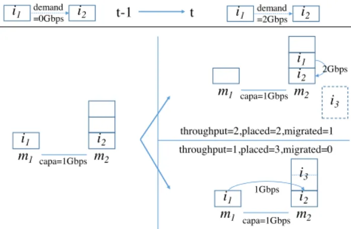
These objectives tend to compete with each other. Indeed, if a task starts communicating with another task, migrating it to the same machine (or to a machine closer in the topology) can increase the throughput at which they communicate, thus increasing the throughput objective function – but this will incur an increase of the migration cost. Likewise, if a new task arrives at t and
needs important CPU resources, placing it right away could utilize CPU capac-ity that could have been used for co-locating tasks: increasing the placement objective can in some cases decrease the throughput objective.
As an illustration, consider two machines m1 and m2 with CPU capacities
κ1= 1 and κ2= 2, with a bottleneck link (of capacity 1) in between. Assume
that at (t − 1) there were two tasks i1, i2with CPU requirements ri1 = 1 and
ri2 = 1, and that i1 was placed on m1 and i2 on m2. At time t, i1 starts
to communicate with i2 (with throughput demand dti1i2 = 2), and a third
task i3 arrives with CPU requirement ri3 = 2. Then, if one decides to place
this new task, m2 is the only machine with enough capacity to host it. But
placing i3on m2would prevent a migration of i1from m1to m2, which would
have increased the throughput of communication i1 7→ i2. This situation is
summarized in figure 2. m1 i1 m2 i2 capa=1Gbps m1 i1 m2 i2 i3 1Gbps capa=1Gbps m1 m2 i2 i1 i3 2Gbps capa=1Gbps throughput=2,placed=2,migrated=1 throughput=1,placed=3,migrated=0 i1 demand i2 =2Gbps t-1 t i1 demand i2 =0Gbps
Fig. 2 Competition between objective functions
3.4 Linearization
All constraints expressed in section 3.2 are linear with respect to the variables xtimand fiit′(u, v), except for the path enforcement constraint in equation (8).
Exploiting the fact that xt
im∈ {0, 1}, this constraint can be linearized:
fiit′(u, v) ≤ cuv(2 − xtim− xti′m′),
∀(i, i′
) ∈ Ct, ∀m, m′
∈ M, ∀(u, v) ∈ A \ Amm′ (13)
If xt
im× xti′m′ 6= 1, the equation will be fiit′(u, v) ≤ cuv or fiit′(u, v) ≤ 2 cuv,
and will therefore be superseded by equation (4).
The set of constraints can be further compressed by writing only one equa-tion per machine m ∈ M instead of one per tuple m, m′
alter the model but makes the formulation more compact: fiit′(u, v) ≤ cuv 2 − xtim− X m′∈M :(u,v) /∈Amm′ xti′m′ , ∀(i, i′ ) ∈ Ct, ∀m ∈ M, ∀(u, v) ∈ A (14)
In this way, the flow-aware workload migration problem can be expressed as the following multi-objective Mixed Integer Liner Program (MILP):
(P′ ) max T (ft) max P (xt) min M (xt) subject to (1-7), (14) xt∈ {0, 1}It× M ft∈ (R+)Ct×A (15)
4 Flow-Aware Workload Migration 4.1 Resolution Algorithm
This section describes an algorithm (Algorithm 1) solving the previously in-troduced multi-objective MILP (15). This algorithm runs at a given time t representing the “present”. It takes the current inter-application communica-tion requirements and the “past” (from time t − 1) task allocacommunica-tion as inputs, and returning a new allocation as a solution.
A Pareto-optimal approach [30, p. 24] is used: a set of optimal solutions is generated, from which a final solution zt= (xt, ft) can be extracted based
on an operator-defined policy getSolutionFromPolicy(). In the context of this migration model, an allocation z = (x, f) dominates an allocation z′
= (x′
, f′
) if all the objectives functions of the former have better values than the ones of the latter (with at least of one having a strictly better value). That is denoted z ≻ z′ : z ≻ z′ ⇔ P (z) ≥ P (z′) T (z) ≥ T (z′ ) M (z) ≤ M(z′) (P (z), T (z), M(z)) 6= (P (z′ ), T (z′ ), M (z′ )) (16)
A set S = {z1, . . . , zn} of solutions is Pareto-optimal if and only if:
∀z, z′
∈ S, z 6= z′
⇒ (z 6≻ z′
∧ z′
6≻ z) (17)
To generate the set of Pareto-optimal solutions for the multi-objective problem, the ε-constraint method [30, p. 98] is used. It consists of reducing
Algorithm 1Multi-Objective Migration Algorithm
zt−1← input ⊲ initial state Ct, dt
ii′, B, εp, εp← input ⊲ parameters S ← ∅
forεp∈ [εp, εp] with step δpdo forεm∈ [B, 0] with step −δm do
if∃z′∈ S, P (z′) ≥ ε
p∧ M (z′) ≤ εmthen
continue ⊲ dominant solution already existing end if
z ← solution of (18)
⊲ if z is not dominated, it is a candidate solution if6 ∃z′∈ S, z′≻ z then
⊲ remove any existing solution dominated by z for z′∈ S do
if z ≻ z′then S ← S \ {z} end if
end for
S ← S ∪ {z} ⊲ add z to candidate solutions end if
end for end for
⊲ select the best solution according to the considered policy zt← getSolutionFromPolicy(S)
a multi-objective linear programming model to a single-objective model, by relaxing all objective functions but one and considering them as constraints. These constraints are obtained by bounding the relaxed objective function by a number ε that varies in a certain interval. Although its initial formulation only considers two-objectives problems, it can be extended to problems with a greater number of objective functions [32], as it is the case here.
The two functions that are relaxed are the placement objective and the migration cost, because it is simple to grid the corresponding space. The single-objective MILP that results is given by:
(Pε) max T (ft) subject to (1-7), (14) P (xt) ≥ εp M (xt) ≤ ε m xt∈ {0, 1}It ×M ft∈ (R+)Ct ×A (18)
where εp, εmare bounds varying in [εp, εp] and [0, B] respectively.
For the placement objective, a simple upper bound for εp corresponds to
the number of tasks:
εp=
X
i∈It
1 = |It| (19)
Similarly, a lower bound for εp can be easily derived from tasks that were
m1,1 m1,10 s1 ... m2,1 m2,10 s2 ... s0
Fig. 3 Network topology used in the example run
u = s0, v ∈ {s1, s2} cuv= cvu= 40 u ∈ {s1, s2}, v ∈ M cuv= cvu= 40
u ∈ M cuu= 200
Table 2 Link capacities for the example topology
(2), they cannot be forcefully terminated: εp= X i∈It−1∩It X m∈M xt−1im (20)
For the migration cost, correctly choosing the upper bound B for εmhas
a large impact on the running time of the algorithm. This bound B will be referred to as the migration budget.
4.2 Computational Example
In large-scale deployments, the amount of CPU resources is likely sufficient for all tasks to be deployed. However, complex situations can exist, for which it is beneficial to have an understanding of the implications that different allocation choices can have. For instance, when new tasks arrive that have a high CPU requirement, choosing to place them upfront can consume CPU capacity which could have been used to migrate a smaller task and satisfy its throughput demand. This section illustrates the model response in situations where placement and migration are competing with each other, by way of an environment in which the machines are nearly overloaded in the initial state. The algorithm has been implemented in Python using the Gurobi MILP solver [33], and all the simulations have been run on a virtual machine with 4 GB of RAM and an 2.6 GHz CPU.
4.2.1 Simulation Parameters
A simple two-tier tree topology is used, consisting of one root switch s0linked
to two ToR switches s1, s2, each linked to 10 machines (Figure 3). In order
0 1 2 3 4 41 42 43 44 45 46 47 48 49 50 710 720 730 740 750 760 770 780 790 T h ro u g h p u t Total DC throughput Pareto-optimal solutions Migrated Placed T h ro u g h p u t 710 720 730 740 750 760 770 780 790
Fig. 4 Multi-objective model example run: solutions and Pareto-optimal solutions.
higher throughput, each machine has a link to itself, with a higher capacity than other links in the data center, as depicted in Table 2.
The CPU capacity is set to 3 for each machine – which gives a total capacity of 60. An initial state with 40 tasks of size ri = 1 and a throughput demand
graph Gt−1d with 80 arcs of intensity dt−1ii′ = 10 is considered, with an initial
allocation zt−1 optimal with respect to throughput demands3
.
Given this allocation, this study explores the model behavior when com-munication demands of existing tasks change, while new bigger tasks arrive in the system. Communication demand changes are modeled by adding 10 ran-dom arcs (of intensity dt
ii′ = 10) between the already running tasks. Arrival of
new tasks is modeled by creating 10 new tasks of size ri = 2, and by adding
10 random arcs (of intensity dt
ii′ = 5) going out of these tasks.
4.2.2 Results
In order to obtain the set of Pareto-optimal solutions S at time t, one iteration of Algorithm 1 was run. Figure 4 shows a three-dimensional representation of the solutions computed for one of those runs: Pareto-optimal solutions can be visually identified as those for which no other solutions have better coordinates in all dimensions. Results show that non-trivial behavior occurs when the data center is almost fully loaded: while placing a few new tasks improves the overall throughput, allocating all of them has a detrimental effect on the overall throughput because it prevents migration of other tasks.
This shows the interest of using a multi-objective model in cases where the objectives are conflicting with each other.
3
zt−1 is obtained by starting from a random state and solving (15) where only the throughput objective is considered, with the additional constraint that all tasks must be allocated.
Algorithm 2Heuristic Multi-Objective Resolution
zt−1← input ⊲ initial state Ct, dt
ii′, B ← input ⊲ parameters m ← 0 ⊲ total migration cost ∆ ← input ⊲ incremental budget
ˆ S ← ∅ ˆz0← zt−1
τ ← 1 ⊲ step index whilem < B do
⊲ reduce ∆ at last iteration so that m + ∆ ≤ B ∆ ← min{∆, B − m}
⊲ find an allocation within ∆ of the previous one
ˆzτ ← solution of max T (ˆfτ) subject to (1-7), (14) with t 7→ τ P (ˆxτ) = |I| M (ˆxτ, ˆxτ −1) ≤ ∆ ˆ xτ ∈ {0, 1}I×M ˆfτ∈ (R+)Ct ×A ifM (ˆxτ, ˆxτ −1) = 0 then
break ⊲ stop if no task could be migrated end if
ˆ
S ← ˆS ∪ {ˆzτ}
⊲ compute the migration cost w.r.t. initial state m ← M (ˆxτ, ˆx0)
τ ← τ + 1 end while
zt← getSolutionF romP olicy( ˆS) return zt
5 Pareto Front Approximation
Section 4 introduced a generic solution approach, which allows to compute the exact Pareto front for the three competing objectives (placing the high-est number of tasks, minimizing the cost incurred by migration, achieving the best inter-application throughput) by means of an ε-constraint method. Al-though this approach generates an exact set of efficient solutions, and thus can be useful for small and highly-constrained deployments, its computational complexity makes it unsuitable to model larger infrastructures.
In order to overcome this issue, this section derives and experimentally analyses a heuristic for approximating the Pareto front. Section 5.1 introduces the approximation method, and section 5.2 provides the results of computa-tional experiments in order to validate the quality of the proposed approach.
5.1 Heuristic Formulation
In large deployments, it is assumed that there are enough resources to accom-modate all tasks to be run, thus the remainder of this section assumes that all tasks can be placed (i.e. that there exists at least one solution to (18) such
u = s0, v ∈ {s1, . . . , sk} cuv= cvu= 40 u ∈ {s1, . . . , sk}, v ∈ M cuv= cvu= 40
u ∈ M cuu= 1000
Table 3 Link capacities for the k-racks topology
that P (x) = |It|). In order to focus on migration, it is also assumed that no
new task arrives (i.e. It= It−1:= I).
Given this assumption, a heuristic allowing to approximate the Pareto front in the throughput-migration plane, i.e. for (P (z), T (z), M(z)) ∈ {|I|} × [0, +∞) × [0, B], is introduced. The issue with the ε-constraint approach intro-duced in section 4 is that, when considering the migration of B tasks, there are O(|I|B|M |B) possible recombinations, which can be computationally
expen-sive. In order to limit the combinatorics of the recombination, the introduced heuristic splits the migration process in smaller chunks, considering fewer mi-grations at a time, and proceeding in a greedy way until the total budget is exhausted, as described in Algorithm 2.
For clarity, let M (xt, xt′
) represent the migration cost when going from state xtto xt′ : M (xt, xt′) = X i∈I∩It′ X m∈M sixt ′ im(1 − xtim) (21)
Let ∆ > 0 be a parameter representing an incremental budget. Starting from an initial configuration zt−1, and given an upper-bound B on the migration cost,
intermediary states (ˆz0
= zt−1, ˆz1
, . . . , ˆzτ, . . . , ˆzτ) are created. At each step
τ ≥ 1, a new placement is generated by maximizing the throughput objective, with the constraint that no more than ∆ is incurred as a migration cost as compared to step (τ −1). This way, no more than O(|I|∆|M |∆) recombinations
are considered at each step, allowing for a smaller expected computational complexity. This process ends when no further tasks can be migrated, or when a total migration cost of B (as compared to step 0) has incurred. The heuristic tracks of the solutions generated while generating the successive solutions, so as to build an approximate Pareto front ˆS.
5.2 Computational Experiments
This section experimentally illustrates the benefits of using the Pareto front approximation heuristic, both in terms of computational complexity and qual-ity of the approximation. The sensitivqual-ity of the heuristic to the incremental budget parameter ∆ is also experimentally explored. The experimental plat-form is the same as in section 4.2.
5.2.1 Simulation Parameters
In a common data center, all machines in a rack are linked to a top-of-rack (ToR) switch, and those ToR switches are linked to each other via an
aggrega-tion router. In data centers, several such configuraaggrega-tions can be linked together thanks to a third routing layer – in all cases, resulting in a tree-like topology. For the purposes of these simulations, a k-racks topology is defined as a tree where a core switch s0is attached to k ToR switches s1, s2, . . . , sk. Each
ToR switch sh (1 ≤ h ≤ k) is attached to 10 machines mh,1, mh,2, . . . , mh,10.
This topology thus comprises 10 × k machines, and Figure 3 depicts a 2-racks topology. Links capacities are set as per Table 3, i.e. links between the core switch and the ToR switches, and between the ToR switches and the machines have a capacity of 40. Loopback interfaces on the machines have a capacity of 1000 – so as to favor placement of tasks which communicate with each other on the same machine.
Five k-racks topologies are considered, for k ∈ {2, 3, 4, 5, 10} (for a corre-sponding number of machines |M | ∈ {20, 30, 40, 50, 100}). For each of these topologies, four scenarios are considered with different tasks-per-machine ra-tios, such that |I| ∈ {|M |, 2|M |, 5|M |, 10|M |} – as a way to compare between different load factors for the machines. This makes for a total of 5 × 4 = 20 scenarios.
CPU requirements of tasks are set to ri = 1, and CPU capacities of the
machines to κm= 20. This allows for up to 20 tasks per machine, thus ensuring
that all tasks can always be placed. To simplify understanding the migration cost, tasks size (for computing the migration cost) are set to si = 1, thus
the migration cost simply becomes the number of migrated tasks. Tasks are initially uniformly randomly assigned to the machines. The communication matrix is generated by: (i) for each task i ∈ I, uniformly choosing a random number di of destinations in {1, 2, 3}, (ii) for each of these di destinations,
uniformly choosing a task i′ ∈ I \ {i} and (iii) setting a throughput demand
dii′ for the communication i 7→ i′ uniformly in {1, 2, . . . , 10}.
For each of these 20 scenarios, the exact Pareto front is computed using Algorithm 1, with a migration budget (maximum migration cost) B = 30. The approximate Pareto front as described in Algorithm 2 is computed for five different values of the incremental budget ∆ ∈ {1, 2, 3, 4, 5}.
5.2.2 Comparative Results
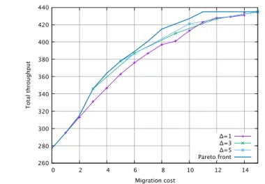
In order to illustrate the results, the cases of the 2-racks topology (20 machines) with 40 and 100 tasks are first considered as examples. For these two cases, Figures 5 and 6 depict the generated exact and approximate Pareto fronts. Those figures show the different solutions from among which one can be choose, after running either algorithm. As depicted in the figures, migrating more tasks obviously increases the migration cost – while enabling communicating tasks to be co-located, hence increasing the total achievable throughput.
Depending on requirements, a solution can be chosen from the Pareto-optimal set that offers a tradeoff between improving the overall throughput and incurring more migrations. In these two examples, it can be observed that the approximate Pareto fronts generated by algorithm 2 for ∆ ≥ 3 closely
260 280 300 320 340 360 380 400 420 440 0 2 4 6 8 10 12 14 T o ta l th ro u g h p u t Migration cost Δ=1 Δ=3 Δ=5 Pareto front
Fig. 5 Pareto front approximation: Exact Pareto front and approximate Pareto fronts from Algorithm 2 for ∆ ∈ {1, 3, 5}. Tree topology, 20 machines, 40 tasks.
500 550 600 650 700 750 800 850 900 950 1000 0 5 10 15 20 25 30 T o ta l th ro u g h p u t Migration cost Δ=1 Δ=3 Δ=5 Pareto front
Fig. 6 Pareto front approximation: Exact Pareto front and approximate Pareto fronts from Algorithm 2 for ∆ ∈ {1, 3, 5}. Tree topology, 20 machines, 100 tasks.
follow the exact front. It can also be observed that for ∆ = 1, results are of lower quality, and that in the example of Figure 6, the algorithm was unable to find solutions for more than 24 migrations.
In order to quantify the impact of these algorithms on the quality of the obtained solution set, let θ20 (resp. θ0, θ30) represent the throughput
corre-sponding to a migration cost of 20 (resp. 0, 30) in the Pareto front. More formally, this means that θ20 is the coordinate such that (|I|, θ20, 20) ∈ S; for
instance, in Figure 6, θ20 = 876 for the exact Pareto front. Figure 7 (resp. 8)
1 1.2 1.4 1.6 1.8 2 2.2 2 0 -2 0 3 0 -3 0 1 0 0 -1 0 0 0 5 0 -5 0 0 3 0 -3 0 0 2 0 -2 0 0 4 0 -4 0 0 2 0 -4 0 1 0 0 -5 0 0 2 0 -1 0 0 5 0 -5 0 4 0 -4 0 5 0 -2 5 0 1 0 0 -2 0 0 1 0 0 -1 0 0 3 0 -1 5 0 4 0 -2 0 0 5 0 -1 0 0 3 0 -6 0 4 0 -8 0 T h ro u g h p u t im p ro v e m e n t Topology (#machines-#tasks) Δ=1 Δ=2 Δ=3 Δ=4 Δ=5 Exact
Fig. 7 Pareto front approximation: throughput improvement for 20 migrations θ20/θ0. Exact Pareto front vs approximate Pareto fronts from Algorithm 2 for ∆ ∈ {1, 2, 3, 4, 5}. 20 different scenarios. 1 1.2 1.4 1.6 1.8 2 2.2 2.4 2 0 -2 0 3 0 -3 0 1 0 0 -1 0 0 0 5 0 -5 0 0 3 0 -3 0 0 2 0 -2 0 0 4 0 -4 0 0 2 0 -4 0 1 0 0 -5 0 0 2 0 -1 0 0 5 0 -5 0 4 0 -4 0 5 0 -2 5 0 1 0 0 -2 0 0 1 0 0 -1 0 0 3 0 -1 5 0 4 0 -2 0 0 5 0 -1 0 0 3 0 -6 0 4 0 -8 0 T h ro u g h p u t im p ro v e m e n t Topology (#machines-#tasks) Δ=1 Δ=2 Δ=3 Δ=4 Δ=5 Exact
Fig. 8 Pareto front approximation: throughput improvement for 30 migrations θ30/θ0. Exact Pareto front vs approximate Pareto fronts from Algorithm 2 for ∆ ∈ {1, 2, 3, 4, 5}. 20 different scenarios.
narios, for the exact Pareto front as well as the approximate Pareto fronts. This represents the relative improvement in terms of overall throughput if the operator chooses to migrate 20 (resp. 30) tasks after inspecting the set of Pareto-optimal solutions. It appears that, for ∆ ≥ 2, the achievable through-put improvement when using the heuristic method introduced in section 5.1 is close to the exact solution. Overall, choosing ∆ = 5 yields the better results: for 20 migrations, the results are better in all the twenty tested instances, and for 30 migrations they are outperformed by ∆ = 4 in only three instances. For
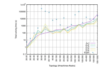
0.1 1 10 100 1000 10000 100000 1x10⁶ 2 0 -2 0 3 0 -3 0 2 0 -4 0 4 0 -4 0 3 0 -6 0 5 0 -5 0 2 0 -1 0 0 4 0 -8 0 3 0 -1 5 0 5 0 -1 0 0 2 0 -2 0 0 4 0 -2 0 0 5 0 -2 5 0 1 0 0 -1 0 0 3 0 -3 0 0 1 0 0 -2 0 0 4 0 -4 0 0 5 0 -5 0 0 1 0 0 -5 0 0 1 0 0 -1 0 0 0 T o ta l s o lv in g t im e ( s ) Topology (#machines-#tasks) Δ=1 Δ=2 Δ=3 Δ=4 Δ=5 Exact
Fig. 9 Pareto front approximation: time to generate the approximate Pareto front, for up to B = 30 migrations. Exact Pareto front (Algorithm 1) vs approximate Pareto fronts (Algorithm 2) for ∆ ∈ {1, 2, 3, 4, 5}. 20 different scenarios.
∆ = 5, the throughput improvement remains within a 3% error as compared to the exact solution after 20 migrations, and within a 5% error after 30 mi-grations. Using ∆ = 1 yields results of lower quality, because the algorithm is not able to explore reconfigurations with two migrations at the same time (i.e. swapping tasks), and because it can terminate prematurely if the through-put cannot be improved by migrating only one task. For 20 migrations, ∆ = 3 also yields results of lower quality, but this is more of an artificial nature: the number of migrations considered is 18 instead of 20 (since 20 is not a multiple of 3).
Finally, Figure 9 depicts the time needed to generate the exact and ap-proximate Pareto fronts. While computing the exact Pareto front is very time-consuming, the approximation heuristics introduced reduces the required computation time. Overall, the lowest computation times are achieved for ∆ ∈ {3, 4, 5}, whereas ∆ ∈ {1, 2} exhibit higher running times. The choice ∆ = 5, which can be observed to exhibit the best results, in terms of through-put improvement, in the majority of cases – with a comthrough-putation time con-stantly better than the reference exact approach, performing approximately one order of magnitude faster when B = 30 (from 5.1× faster for 100 machines and 200 tasks, to 1800× faster for 30 machines and 60 tasks).
To conclude, the approximation method presented in section 5.1 can greatly reduce the time needed to compute a set of approximate Pareto optimal solu-tions, while generating solutions close enough to the exact ones. It is realistic to note that, although an improvement in solving time is observed regardless of the topology size, Figure 9 suggests that using a MILP approach (exact or approximate) might be unfit for too large topologies.
6 Conclusion
In data centers, applications may exhibit time-varying communications de-pendencies, and migrating tasks in such environments can be a means to re-distribute the load over the whole infrastructure, while optimizing inter-task communications. In this paper, a linear programming framework is introduced, which represents the data center topology, and communications dependencies between workloads. Using this framework, a multi-objective model is devel-oped, which, when solved, can propose a reorganization of workloads so as to (i) place the highest number of new tasks, (ii) maximize the overall achievable throughput, and (iii) minimize the migration cost, incurred by this reorgani-zation.
The approach developed is generic with respect to the network topology and the inter-application communication demands, and is novel in that, when compared to other workload migration frameworks, it generates a set of Pareto-optimal solutions. From among this solution set, a workload allocation can be chosen, which yields the best tradeoff in terms of throughput improvement versus the cost incurred by task migration. A solution algorithm using the ε-constraint method is proposed as a baseline. Then, a heuristic is presented, which generates an approximate Pareto front. Computational experiments on different topologies show that the proposed approximation builds solutions close to the optimal Pareto front, while greatly reducing the computation time.
Having shown the desirability of considering inter-application dependencies in migration models, an interesting question that arises is how the proposed model can be extended to take into account more fine-grained parameters. These could include the distance between source and destination hosts when migrating, the energy cost induced by machines which are on or off, and the possibility to load-balance flows across multiple paths.
References
1. Christopher Clark, Keir Fraser, Steven Hand, Jacob Gorm Hansen, Eric Jul, Christian Limpach, Ian Pratt, and Andrew Warfield. Live migration of virtual machines. In Proceedings of the 2nd conference on Symposium on Networked Systems Design & Implementation-Volume 2, pages 273–286. USENIX Association, 2005.
2. Raffaele Bolla, Marco Chiappero, Riccardo Rapuzzi, and Matteo Repetto. Seamless and transparent migration for tcp sessions. In Personal, Indoor, and Mobile Radio Communication (PIMRC), 2014 IEEE 25th Annual International Symposium on, pages 1469–1473. IEEE, 2014.
3. Shripad Nadgowda, Sahil Suneja, Nilton Bila, and Canturk Isci. Voyager: Complete container state migration. In Distributed Computing Systems (ICDCS), 2017 IEEE 37th International Conference on, pages 2137–2142. IEEE, 2017.
4. Dazhao Cheng, Changjun Jiang, and Xiaobo Zhou. Heterogeneity-aware workload place-ment and migration in distributed sustainable datacenters. In Parallel and Distributed Processing Symposium, 2014 IEEE 28th International, pages 307–316. IEEE, 2014. 5. Deze Zeng, Lin Gu, and Song Guo. Cost minimization for big data processing in
geo-distributed data centers. In Cloud Networking for Big Data, pages 59–78. Springer, 2015.
6. Vivek Shrivastava, Petros Zerfos, Kang-Won Lee, Hani Jamjoom, Yew-Huey Liu, and Suman Banerjee. Application-aware virtual machine migration in data centers. In INFOCOM, 2011 Proceedings IEEE, pages 66–70. IEEE, 2011.
7. Daochao Huang, Yangyang Gao, Fei Song, Dong Yang, and Hongke Zhang. Multi-objective virtual machine migration in virtualized data center environments. In Com-munications (ICC), 2013 IEEE International Conference on, pages 3699–3704. IEEE, 2013.
8. Theophilus Benson, Aditya Akella, and David A Maltz. Network traffic characteristics of data centers in the wild. In Proceedings of the 10th ACM SIGCOMM conference on Internet measurement, pages 267–280. ACM, 2010.
9. Srikanth Kandula, Sudipta Sengupta, Albert Greenberg, Parveen Patel, and Ronnie Chaiken. The nature of data center traffic: measurements & analysis. In Proceedings of the 9th ACM SIGCOMM conference on Internet measurement conference, pages 202–208. ACM, 2009.
10. Xiaoqiao Meng, Vasileios Pappas, and Li Zhang. Improving the scalability of data center networks with traffic-aware virtual machine placement. In INFOCOM, 2010 Proceedings IEEE, pages 1–9. IEEE, 2010.
11. Katrina LaCurts, Shuo Deng, Ameesh Goyal, and Hari Balakrishnan. Choreo: Network-aware task placement for cloud applications. In Proceedings of the 2013 conference on Internet measurement conference, pages 191–204. ACM, 2013.
12. Mohammad Al-Fares, Sivasankar Radhakrishnan, Barath Raghavan, Nelson Huang, and Amin Vahdat. Hedera: Dynamic flow scheduling for data center networks. In NSDI, volume 10, pages 19–19, 2010.
13. Tiago C. Ferreto, Marco A.S. Netto, Rodrigo N. Calheiros, and César A.F. De Rose. Server consolidation with migration control for virtualized data centers. Future Gener-ation Computer Systems, 27:1027–1034, 2011.
14. Chaima Ghribi, Makhlouf Hadji, and Djamal Zeghlache. Energy efficient VM schedul-ing for cloud data centers: Exact allocation and migration algorithms. In 2013 13th IEEE/ACM International Symposium on Cluster, Cloud, and Grid Computing. IEEE, 2013.
15. Hao Jin, Tosmate Cheocherngngarn, David Levy, Alex Smith, Deng Pan, Jiangchuan Liu, and Niki Pissinou. Joint host-network optimization for energy-efficient data center networking. In Parallel & Distributed Processing (IPDPS), 2013 IEEE 27th Interna-tional Symposium on, pages 623–634. IEEE, 2013.
16. Ning Liu, Ziqian Dong, and Roberto Rojas-Cessa. Task and server assignment for re-duction of energy consumption in datacenters. In Network Computing and Applications (NCA), 2012 11th IEEE International Symposium on, pages 171–174. IEEE, 2012. 17. Dhaemesh kakadia, Nandish Kopri, and Vasudeva Varma. Network-aware virtual
ma-chine consolidation for large data centers. In NDM ’13 Proceedings of the Third Inter-national Workshop on Network-Aware Data Management. ACM (6), 2013.
18. Raja Wasim Ahmad, Abdullah Gani, Siti Hafizah Ab. Hamide, Muhammada Shiraz, Abdullah Yousafzai, and Feng Xia. A survey on virtual machine migration and server consolidation frameworks for cloud data centers. Journal of Network and Computer Applications, 52:11–25, 2015.
19. Fabio López Pires and Benjamin Báran. Virtual machine placement literature review. arXiv:1506.01509v1, cited 4 June 2015.
20. Md Hasanul Ferdaus, Manzur Murshed, Rodrigo N Calheiros, and Rajkumar Buyya. Network-aware virtual machine placement and migration in cloud data centers. Emerg-ing Research in Cloud Distributed ComputEmerg-ing Systems, 42, 2015.
21. Zoha Usmani and Shailendra Singh. A survey of virtual machine placement techniques in cloud data center. Procedia Computer Science, 78:491–498, 2016.
22. Weiwei Fang, Xiangmin Liang, Shengxin Li, Chiaraviglio, and Naixue Xiong. VMPlan-ner: Optimizing virtual machine placement and traffic flow routing to reduce network power costs in cloud data centers. Computer Networks, 57(1):179–196, 2013.
23. Tao Chen, Xiaofeng Gao, and Guihai Chen. Optized virtual machine placement with traffic-aware balancing in data ceter networks. Scientific Programming, 6:10 pages, 2016.
24. Shuo Fang, Renuga Kanagavelu, Bu-Sung Lee, Chuan Heng Foh, and Khin Mi Mi Aung. Power-efficient virtual machine placement and migration in data centers. In 2013 IEEE International Conference on Green Computing and Communications and IEEE Inter-net of Things and IEEE Cyber, Physical and Social Computing, pages 1408–1413. IEEE Computer Society, 2013.
25. Jing Xu and José A.B. Fortes. Multi-objective virtual machine placement in virtual-ized data center environments. In 2010 IEEE/ACM International Conference on Green Computing and Communications & 2010 IEEE/ACM International Conference on Cy-ber, Physical and Social Computing, pages 179–188. IEEE Computer Society, 2010. 26. Jing Xu and José A.B. Fortes. A multi-objective approach to virtual machine
manage-ment in datacenters. In Proceeding ICAC’11 Proceedings of the 8th ACM international conference on Autonomic computing, pages 225–234. ACM New York, NY, USA, 2011. 27. Yongquiang Gao, Haibing Guan, Zhengwei Qi, Yang Hou, and Liang Liu. A multi-objective ant colony system algorithm for virtual machine placement in cloud comput-ing. Journal of Computer and System Sciences, 79:1230–1242, 2013.
28. Fabio López Pires and Benjamin Báran. Multi-objective virtual machine placement with service level agreement. In 2013 IEEE/ACM 6th International Conference on Utility and Cloud Computing, pages 203–210. IEEE Computer Society, 2013.
29. Fabio López Pires and Benjamin Báran. Virtual machine placement. A multi-objective approach. In Latin American Symposium of Infrastructure, Hadward, and Software, pages 77–84. IEEE, 2013.
30. Matthias Ehrgott. Multicriteria optimization. Springer Science & Business Media, 2006. 31. Ravindra K Ahuja, Thomas L Magnanti, James B Orlin, and MR Reddy. Applications of network optimization. Handbooks in Operations Research and Management Science, 7:1–83, 1995.
32. Marco Laumanns, Lothar Thiele, and Eckart Zitzler. An adaptive scheme to generate the pareto front based on the epsilon-constraint method. In Dagstuhl Seminar Proceedings. Schloss Dagstuhl-Leibniz-Zentrum für Informatik, 2005.
33. Inc. Gurobi Optimization. Gurobi optimizer reference manual, 2015.
View publication stats View publication stats
Powered by TCPDF (www.tcpdf.org) Powered by TCPDF (www.tcpdf.org)