Hedge Fund Returns and Factor Models: A
Cross-Sectional Approach
∗Serge Darolles† Gulten Mero‡ June 10, 2011
Abstract
This paper develops a dynamic approach for assessing hedge fund risk exposures. First, we focus on an approximate factor model frame-work to deal with the factor selection issue. Instead of keeping the number of factors unchanged, we apply Bai and Ng (2002) and Bai and Ng (2006) to select the appropriate factors at each date. Sec-ond, we take into account the instability of asset risk profile by using rolling period analysis in order to estimate hedge fund risk exposures. Individual hedge fund returns instead of index returns are employed in the empirical application to go further in the comprehension of the covariation structure of the data. In particular, the common behavior of hedge fund returns is filtered not only from the past historical data (time-series dimension), but also from the cross-section of returns. Fi-nally, we apply our approach to equity hedge funds and replicate the returns of the aggregated index.
JEL classification: C52, G12
Key words: Factor model, asymptotic tests, large panel data, risk dimension, replicating portfolio, missing factors.
∗Accepted for publication at Bankers, Markets & Investors (may-june 2011). We thank
our referees for useful comments and suggestions.
†LYXOR AM and CREST-INSEE, France, [email protected]
‡University of Evry, EPEE and CREST-INSEE, France, [email protected]
1
Introduction
In the last two decades, interest in hedge funds from both academics and investors has grown dramatically. These funds are typically organized as pri-vate investment vehicles for wealthy individuals and institutional investors. Since they do not have to disclose their activities publicly, little is known about the risk in hedge fund strategies. The lack of transparency and the fear for style drift have raised the question whether it is possible to iden-tify and estimate the risk factors driving hedge fund returns. Factor models are employed to capture their main characteristics and thus identify the risk exposures.
These models are initially developed to explain common risk affecting eq-uity returns. They are a natural extension of the one-factor CAPM [Sharpe (1964), Lintner (1965) and Black (1972)] and use a set of observed variables, such as market indexes and economic indicators, as proxies for common risk factors. The growth of the hedge fund industry has reoriented the asset pric-ing efforts toward alternative returns offered by hedge funds. For example, Fung and Hsieh (2004) showed that equity-oriented hedge fund indexes have two major exposures: the equity market as a whole, and the spread between small cap and large cap stocks1
.
An extensive literature has documented that hedge fund returns differ from those of the traditional assets. Mutual funds returns have high and positive correlation with asset class returns, which suggests that they be-have as a "buy and hold" strategy. Hedge fund returns seem to be-have low and sometimes negative correlation with traditional asset class returns2
. This
1
As proxied by the difference between the Wilshire Small Cap 1750 and the Wilshire Large Cap 750 index.
2
Note that several recent studies have challenged the absence of correlation of hedge fund returns with market indexes, arguing that the standard methods of assessing their risks may be misleading. For example, Asness et al. (2001) show that in several cases
suggests that they behave as if deploying a dynamic strategy including short sells and leverage. Nonlinear payoffs and time-varying exposures to risk factors are some resulting stylized facts [see Fung and Hsieh (1997a) Fung and Hsieh (1997b), Fung and Hsieh (2001), Fung and Hsieh (2002), Mitchell and Pulvino (2001), Agarwal and Naik (2001) and Agarwal and Naik (2004) among others]. It follows that to analyze hedge fund returns, one has to take into account that their risk exposures are nonlinear and likely to change very frequently. For example, Agarwal and Naik (2004) introduce option-based factors to capture nonlinear payoffs of hedge fund strategies and show that left-tail risk is a priced factor. Fung and Hsieh (1997a) focus on the time-varying risk exposures of hedge funds and show that the Trend Follower index returns are positively correlated with the stock market in situations of bullish markets and negatively correlated in bear markets. Hasanhodzic and Lo (2007) use observed factors, such as the S&P 500 index, the USD return index, the Bond Index, etc., to model the returns of individual hedge funds3
. They estimate the risk exposures using a 24-month rolling window. This methodology has one main drawback: the factor model specification is determined in advance and is kept unchanged through the entire sample period4
. This factor selection mechanism5
does not take into account the time-varying risk profile of hedge fund returns. Therefore, hedge fund anal-ysis should consider that, for different rolling periods, a given investment where hedge funds purport to be market neutral, including both contemporaneous and lagged market returns as regressors and summing the coefficients yield significantly higher market exposure.
3
Note that an alternative approach to observed factor models consists in using option-based factors to capture the nonlinearity of hedge fund returns. For example, ? show that the returns from trend following strategies can be replicated by a dynamically managed option-based strategy known as "lookback option". However, Amin and Kat (2003) point out that option-based models is difficult to be implemented in practice.
4
In other words, their factor selection mechanism consists in selecting a given set of observed factors and keeping it unchanged through the entire period.
5
strategy may not be exposed to the same risk factors.
The factor selection problem is not new in the literature. The main issue is related to the delicate balance between using too many or too few fac-tors. Specifically, adding too many factors lowers the regressors efficiency. Working with too few factors also has an important hidden cost: the model risk. This raises the question whether it is possible to build a factor selection methodology allowing to consider only the appropriate factors. In this paper, we develop a dynamic factor-based approach to explain hedge fund returns. First, we focus on an approximate factor model framework to deal with the factor selection issue. Instead of determining in advance which factors to in-clude in the analysis, we use asymptotic developments of Bai and Ng (2002) and Bai and Ng (2006) to select the relevant factors. We estimate the risk dimension, i.e. the optimal number of latent factors, using individual hedge fund returns. Then, we asses the economic interpretation of these factors by matching them with the observed variables. We thus identify which economic forces drive hedge fund returns. Second, we take into account the instability of asset risk profile by using rolling period analysis to estimate time-varying hedge fund risk exposures. Individual hedge fund returns are used instead of index returns. This choice allows us to go further in the comprehension of the latent factor structure. The information on the common behavior of fund returns is filtered not only from the past historical data (time-series dimension), but also from the cross-section of fund returns. The asymptotic tests we perform hereafter are consistent for large cross-section and moder-ately large time-series dimension. This data configuration is clearly more in line with the dynamic factor selection objective we aim at. Moreover, Chan et al. (2005) point out that a disaggregated approach may yield additional insights not apparent from index-based risk models.
Finally, we use the HFR database to test our approach on a set of indi-vidual equity hedge funds. One possible application of risk factor models is hedge fund replication. This is a challenge that has naturally appeared in response to drawbacks inherent to these funds such as opacity, lack of liq-uidity and high incentive fees. Repliquants generate hedge-fund-like returns using more liquid assets such as market indexes. This allows to construct benchmarks and then get a better evaluation of alpha generation for a given fund. We use hedge fund replication as a criterion for assessing the quality of the dynamic factor-based approach developed herein, as well as the ben-efits of dynamic factor selection mechanism. We find that the hedge fund clone index constructed by our methodology outperforms the "naive" clone index constructed by a methodology consisting of a static and ad hoc factor selection, as in Hasanhodzic and Lo (2007).
The paper is organized as follows. In section 2, we propose a statistic model for large panel data and describe how recent asymptotic tests can be used to assess the common risk structure of asset returns. Section 3 deals with the economic interpretation of the latent factors. Section 4 describes our dynamic factor-based approach to analyze hedge fund returns and discuss the empirical results. Section 5 concludes.
2
Determining the number of latent factors
In this section, we focus on the approximate factor model framework and use Bai and Ng (2002) asymptotic tests to estimate the risk dimension.
2.1 An approximate factor model for hedge fund returns
When dealing with large panel data, the arbitrage pricing theory (APT) of Ross (1976) assumes that a small number of factors can be used to explain
a large number of asset returns. Let Xit be the observed return for fund ith
at time t, for i = 1, ..., N and t = 1, ..., T . We consider the following model with r common factors:
Xit = λ
′
iFt+ eit, (2.1)
where Ft is a r × 1 vector of common factors, λi is a r × 1 vector of factor
loadings for the fund i, and eit is the ith element of the tth column of the
idiosyncratic component matrix. λ′iFt represents the common component of
Xit. The idiosyncratic components are supposed to have zero mean.
We place our analysis in an approximate factor model framework in the sense of Bai and Ng (2002) which is more realistic in hedge fund world, since it allows for weak time and cross-section dependence and heteroscedasticity in the idiosyncratic components. The factors, their loadings, as well as the idiosyncratic errors are not observable and have to be estimated. Although it seems appealing to assume one factor, there is growing evidence against the adequacy of a single factor model in explaining hedge fund returns. For example, Fung and Hsieh (1997a) and Fung and Hsieh (1997b) show that hedge fund risk exposures are multidimensional and highly dynamic. Thus, instead of restricting the analysis by fixing r = 1, we propose a procedure to determine the appropriate number of factors6
.
Determining the number of factors in approximate factor models is an important issue when dealing with large panel data in both cross-sectional (N ) and time-series (T ) dimension. In classical factor analysis [see Ander-son1 (1984)], N is assumed fixed, the factors are independent of errors etand
the covariance matrix of the idiosyncratic components Σ is diagonal. Under
6
The restriction r = 1 is implicitly made when we restrict the analysis to a single index built on hedge fund returns. We use the cross-section dimension to estimate this number from the data.
these assumptions, a root-T consistent and asymptotically normal estimator of Σ as measured by the sample covariance matrix can be obtained. In gen-eral, the classical factor analysis applies to the case of large N but fixed T since the N × N problem can reformulated as a T × T problem, as discussed by Connor and Korajczyk (1993) among others.
Inference on r under classical assumptions is based on the eigenvalues of ˆΣ. Indeed, if a data panel allows for a r factor representation, the first r largest eigenvalues of the N × N covariance matrix of Xt diverge as N
increases to infinity but the (r + 1)th eigenvalue is bounded [see for exam-ple Chamberlain and Rothschild (1983)]. However, it can be shown that all nonzero eigenvalues of bΣ (not just the first r) increase with N , which invali-dates tests based on the sample eigenvalues. A likelihood ratio test can also, in theory, be used to estimate the number of factors under the assumption that eit is normally distributed. But as discussed by Dhrymes et al. (1984),
the number of statistically significant factors estimated by the likelihood test ratio increases with N even if the true number of factors is fixed. Connor and Korajczyk (1993) develop a test for the number of factors in the asset returns, which is derived under sequential limit assumptions, i.e. N con-verges to infinity with a fixed T , then T concon-verges to infinity. In addition, covariance stationarity and homoscedasticity are crucial for the validity of their test. As discussed by Bai and Ng (2002), the main problem in classical analysis is that the theory does not apply when both N and T go to infinity. This is because consistent estimation of Σ (whether it is an N × N or T × T matrix) is not a well defined problem7
.
To address this issue, Bai and Ng (2002) develop an asymptotic theory for factor models with large panel data (when N , T → ∞). Their analysis
7
For example, when N > T , the rank of bΣis no more than T , whereas the rank of Σ can always be N .
goes beyond the classical factor analysis since: i) the sample size in both the cross-section and time-series dimension have to be taken into account; ii) the factors are not observed. Based on an approximate factor model framework, they first establish the convergence rate for the factor estimates that will allow for consistent estimation of r. They then propose some panel criteria and show that the number of factors can consistently be estimated. Inference on r is set up as a model selection problem and the proposed criteria depend on the trade-off between good fit and parsimony. The penalty for overfitting is a function of both N and T in order to consistently estimate the number of factors. Consequently, the usual AIC and BIC criteria, which are functions of N or T alone, do not work when both dimensions of the panel are large. In addition, their theory holds under heteroscedasticity and weak cross-section and serial dependance in the idiosyncratic components. These additional assumptions are reported in the appendix A. Note that Bai and Ng (2002) approximate factor structure is more general than that of Chamberlain and Rothschild (1983), which focuses only on the cross-section behavior of the data by allowing for weak cross-section dependence.
2.2 Asymptotic tests for estimating the number of latent factors
Equation (2.1) can be written in a more general way as:
X = F Λ′+ e, (2.2)
where X is the T × N matrix of individual hedge fund returns, e is the T x N matrix of idiosyncratic components, Λ is the N × r matrix of factor loadings, and F is the T × r matrix of common factors.
We use the asymptotic principal component method to estimate the fac-tors and their loadings. This method minimizes the following objective func-tion: V (k) = min Λ,Fk(N T ) −1 N X i=1 T X t=1 (Xit− λkiFtk)2, (2.3)
subject to the normalization of either (Λk)′Λk/N = I
k or (Fk)′Fk/T = Ik.
The superscript in λki and Ftk signifies the allowance of k factors in the estimation, with k = min(T, N ). There are two possible solutions:
i) Concentrating out Fkand using the normalization Λk′Λk/N = Ik, the
esti-mated factor loading matrix Λk is√N times the eigenvectors corresponding
to the k largest eigenvalues of the N × N covariance matrix X′X. Given Λk,
Fk= XΛk/N represents the corresponding matrix of the estimated common
factors.
ii) The second solution is given by ( eFk, eΛk), where eFk represents√T times
the eigenvectors corresponding to the k largest eigenvalues of the T × T covariance matrix XX′. The normalization (Fk)′Fk/T = I
k implies that
e
Λk′ = ( eFk)′X/T is the corresponding matrix of the estimated common
fac-tors.
The first solution is less costly when T > N , while the second one is more appropriate when T < N . As it will be discussed later, our dynamic approach uses T -month rolling period estimations, with T smaller than the number of individual hedge funds N . We thus retain the second set of principal component calculations to estimate the factors and their loadings.
r. Let Fk be a matrix of k factors and V (k, eFk) = min Λ 1 N T N X i=1 T X t=1 (Xit− λk ′ i Fetk)2, (2.4)
be the sum of squared residuals when k factors are estimated. Then a loss function V (k, Fk) + kg(N, T ), with g(N, T ) being the penalty for overfitting,
can be used to determine k. The authors propose some penalty functions g(N, T ) such as the following criteria of form IC(k) = V (k, Fk) + kg(N, T ) can consistently estimate r:
IC1(k) = ln(V (k, eFk)) + k( N + T N T ) ln( N T N + T), IC2(k) = ln(V (k, eFk)) + k( N + T N T ) ln C 2 N T, (2.5) IC3(k) = ln(V (k, eFk)) + k( ln CN T2 CN T2 ).
In these equations, CN T = min(√N ,√T ), eF is the matrix of estimated
common factors and V (k, eFk) = N−1PNi=1ˆσ2i, ˆσi2 = eeie˜i/T . The IC1, IC2
and IC3 criteria are called Information Criteria8.
We use Monte Carlo simulations to assess the finite sample properties of IC criteria relative to our data configuration. The simulation procedure is described in the Appendix B. The results reported in Table 3 show that IC2
outperform the other criteria in inferring the appropriate number of factors. Moreover, a small degree of correlation in the idiosyncratic errors does not affect their finite sample properties.
8
Bai and Ng (2002) also propose another set of criteria called Panel Criteria, P C, which present two main drawbacks as compared to IC criteria: i) the P C criteria depend on ˆ
σ2
= V (kmax, ˜Fkmax)and, thus, on the arbitrary choice of kmaxwhich is set to 8; ii) Monte
Carlo simulations performed by Bai and Ng (2002) show that, although asymptotically equivalent, IC criteria outperform P C criteria in terms of finite sample properties. For these reasons, only IC criteria are considered in this study.
3
Economic interpretation of risk exposures
Based on the Bai and Ng (2006) framework, we discuss how to match the latent factors to observed variables. This step is essential to identify which economic forces drive hedge fund returns.
3.1 Matching observed variables to latent common factors
The factors represent the common shocks that are responsible for the covari-ation of asset returns. These common factors are directly determined by the covariance structure of the data9
. It is therefore intuitive to replace the un-observed factors with statistically estimated ones. For example, Lehman and Modest (1988) use factor analysis, while Connor and Korajczyk (1986) and Connor and Korajczyk (1988) adopt the method of principal components. However, these statistic factors do not have direct economic interpretation.
Another possibility is to select a set of observed variables as proxies of the unobserved latent factors. For example, in the CAPM analysis equity index returns are used as proxies of the unobserved market portfolio returns. Chen et al. (1986) find that the factors in the APT are related to macroeconomic variables. Fama and French (1993) propose three well-known observed fac-tors: the market excess return (MKT), the small minus big (SMB), and the high minus low (HML) factors. Later on, Carhart (1997) extends the three factor model of Fama and French (1993) by adding a forth factor in order to take into account risk related to return persistence. Agarwal and Naik (2004) use option-based factors to account for nonlinear returns generated by dynamic investment strategies employed by hedge funds.
It is intuitive to associate the latent factors with the observed variables in
9
The idea to use statistic to price asset returns was first introduced by the arbitrage pricing theory (APT) developed by Ross (1976) and Roll and Ross (1980).
order to facilite the economic interpretation of common variations. However, as pointed out by Shanken (1992), estimation of betas using proxy factors is relevant only if the fundamental factors are spanned by the observed vari-ables. Such a condition is breached even if a pure measurement error is added to a perfect proxy.
Suppose we observe an (m × 1) vector of economic variables, denoted Gt.
We want to figure out whether its elements are generated by (or are linear combinations of) the r latent factors Ft. As discussed in Bai and Ng (2006),
considering Gjt to be an exact linear combination of the latent factors is a
too strong assumption. Even if an observed series can explain the variations of the latent factors very closely, it may not necessarily be an exact factor in a mathematical sense. This is due, for example, to measurement errors and time aggregation [see Breeden et al. (1989)]. For that reason, we consider an approximate relation between the observed and the latent factors:
Gjt = δ′Ft+ ǫjt, (3.1)
where Ft is a r × 1 vector of latent factors and ǫjt∼ N(0, σǫ2(j)).
Bai and Ng (2006) show that the space spanned by the latent factors can consistently be estimated when the simple size is large in both the cross-section and the time series dimensions10
. They develop some criteria to match the observed variables with the estimated latent factors.
3.2 Asymptotic tests
Suppose that we observe Gjt, j = 1, ..., m and t = 1, ..., T . We want to test if
it is generated by (or is a linear combination of) r latent factors. The latent
10
The rate of convergence and the limiting distributions for the estimated factors, factor loadings and common components, estimated by the principal component method (PCA) was developed by Bai and Ng (2003).
factors F and their number r are not observed and have to be estimated. We denote bGjt=bγ
′
jFet, where eFtis the principal component estimation11
of F , bγj is obtained by least squares from a regression of Gjt on eFt, and
bǫjt= Gjt− bGjt. The residualsbǫjtare referred as a measurement error, even
though it might be due to systematic differences between Ft and Gjt.
We consider two statistics proposed by Bai and Ng (2006) to compare the observed variables with the estimated factors eF .
N S(j) = var(d bǫ(j)) d var( bG(j)), (3.2) R2(j) = var( bd G(j)) d var(G(j)), (3.3)
where a consistent estimate of dvar( bGjt) is given by:
1 Nbγ
′
jVe−1ΓetVe−1bγj. (3.4)
In this equation, eV is aer x er diagonal matrix consisting of the er largest eigen-values of sample covariance matrix XX′/N T , and eΓtis a consistent estimate
of Γt = limN −→∞N1 PNi=1PNj=1E(λiλ
′
jeitejt). To allow for heteroskedastic
errors eit, eΓt is given as follows:
e Γt = 1 N N X i=1 ee2iteλieλ ′ i, (3.5)
where eλi and eeit are respectively the factor loadings and the idiosyncratic
errors resulting from the principal component computations as described in section 2.2.
The statistics given in equations (3.2) and (3.3) consider one observed
11
As discussed in the previous section, F and r can consistently be estimated using asymptotic principal component computations when both sample dimensions are large.
variable Gj at a time. The N S(j) statistic represents a noise-to-signal ratio.
If Gj is an exact factor, i.e. Gjt = δ
′
Ft the population value of N S(j) is
zero. Concerning R2(j), the higher this statistic, the higher the adequacy between the observed and the latent factors.
Finally, we use Monte Carlo simulations to assess the finite sample prop-erties of the proposed criteria, as well as their critical values. Simulation procedure is described in the Appendix C. The results reported in Table 5 show that both criteria help identify the appropriate observed factors. In the following section we show how we use these criteria to select the rele-vant observed factors and apply this factor selection procedure to a set of individual equity hedge funds.
4
Empirical applications
In this section, we develop a dynamic factor-based approach to analyze eq-uity hedge fund returns. Subsection 1 describes the data. In subsection 2, we estimate the risk dimension. Subsection 3 provides an economic interpreta-tion of the covariance structure of fund returns, while subsecinterpreta-tion 4 presents the dynamic hedge fund return analysis and discusses the empirical results.
4.1 The data
We use in all this section the HFR database providing returns of individual hedge funds. This database contains only the funds that are still "alive", i.e. active as of the end of our sample period, December 2005. We acknowledge that the database suffers from the survivorship bias. However, the impor-tance of such a bias for our application is tempered by the fact that many successful funds leave the sample as well as the poor performers, reducing the upward bias in expected returns. In particular, Fung and Hsieh (2000)
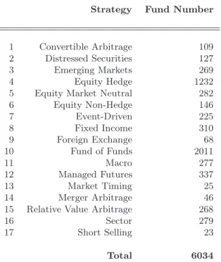
estimate the magnitude of survivorship bias to be 3% per year, and Liang (2000) estimate is 2.24% per year. In addition, the focus of our study is on the relative performance of our dynamic approach versus a naive one which consists in including in the analysis all the available observed factors and keeping this set unchanged. It follows that any survivorship bias should im-pact both approaches in the same way, leaving their relative performances unaffected. HFR database classifies funds into one of 17 different investment styles, listed in Table 6 in the Appendix D.
We limit our analysis to the individual funds of the equity hedge strat-egy for two reasons. First, this stratstrat-egy involves quite homogenous equity-oriented funds investing on both the long and the short sides of the market. Thus, we expect the equity hedge funds to be more sensible to equity-based risk factors. Second, the number of funds N with full set of data for our studying period (January 1997 to December 2005) is large, which will im-prove the finite sample properties of our tests. We drop funds that: i) do not report net-of-fee returns; ii) report returns in currencies other than the U.S. dollar; iii) report returns less frequently than monthly; iv) have less than 10 Million US dollars of assets under management (AUM). These filters yield a final sample of 680 equity hedge funds.
4.2 Estimating the number of latent factors that drive equity hedge fund returns
As discussed in subsection 2.2, Monte Carlo simulation results (see the Ap-pendix B) motivate the use of IC2criterion to estimate the number of latent
factors. Since our study focuses on a dynamic approach, we have to choose the minimal length of the rolling window (T ) ensuring good finite sample properties for the estimated parameters. T depends on the trade-off
be-tween a high dynamics of our approach and good finite sample properties of the Bai and Ng (2002) criteria, in particular IC2. i) If T is too small
the convergence is not achieved and the selected criteria will not yield good estimates of the number of latent factors. ii) If T is too large, our approach will lose its dynamic character.
The results reported in Table 3 in the Appendix B show that for T = 24 the finite sample properties of the six criteria are less precise than for T = 36. For instance, for T = 24 and r = 3 the IC criteria underestimate r. For T = 36, the IC criteria, and in particular IC2, yield the appropriate number
of factors more precisely. We use this choice in all the following empirical applications.
The length of the entire sample allows us to form 72 rolling windows of length 37 months for each one. The first rolling window goes from January 1997 to January 2000, the second from February 1997 to February 2000, ..., the last one extends from December 2002 to December 2005. We use the first 36 months of each rolling window to perform the factor selection procedure and to estimate the beta coefficients, while the last (the 37th) observation is meant to compare hedge fund returns and model predictions12
.
Hedge fund returns are standardized previously within the 36 first months of each rolling period. Let X be the T by N matrix of the equity hedge fund returns of our sample data such that the ith column is the time series of fund i. Let eV be a r × r diagonal matrix consisting of the r largest eigenvalues of XX′/N T . Let eF = ( eF
1, ..., eFT)′ be the principal component estimates
of F under the normalization that FT′F = Ir. Then eF is comprised of the
r eigenvectors (multiplied by√T ) associated with the r largest eigenvalues
12
For each rolling window, we drop the funds that do not have full data for the given period. This allows us to count progressively for the new funds that enter in the database. The size of our sample varies from 97 for the first rolling window to 388 for the last one.
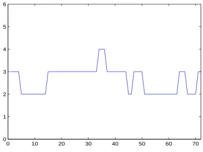
0 10 20 30 40 50 60 70 0 1 2 3 4 5 6
Figure 1: The number of latent factors estimated using IC2 criterion for
each rolling period.
of the matrix XX′/N T in the decreasing order. Let Λ = (λ
1, ..., λN)′ be
the matrix of factor loadings. The principal component estimator of Λ is e
Λ = X′F /T ande ee
it = Xit− eλ′iFet.
Using the principal component estimates, we calculate the IC2 criterion
to estimate the number of latent factors. Figure 1 plots, for each rolling window, the estimated number of factors, which varies between 2 and 4. This result seems to be quite realistic for this kind of strategy and highlights the CAPM shortcomings when explaining hedge fund returns, even for an equity-oriented strategy.
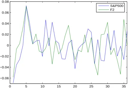
Figures 2 and 3 plot the two first estimated latent factor and the S&P 500 index returns. F 1 and F 2 are the estimated latent factors corresponding to respectively the first and the second largest eigenvalue of the covariance matrix of the fund returns for the last rolling period which extends from December 2002 to December 2005. Since F 1 and F 2 are estimated using
0 5 10 15 20 25 30 35 −0.06 −0.04 −0.02 0 0.02 0.04 0.06 0.08 S&P500 F1
Figure 2: The first estimated latent factor F1 and the S&P 500 index returns from December 2002 to December 2005.
0 5 10 15 20 25 30 35 −0.06 −0.04 −0.02 0 0.02 0.04 0.06 0.08 S&P500 F2
Figure 3: The second estimated latent factor F2 and the S&P 500 index returns from December 2002 to December 2005.
standardized data, we renormalize them in order to obtain the same stan-dard deviation as for S&P 500 index. S&P 500 index returns have been centered by their mean in order to facilitate the comparison with the es-timated latent factors. The correlation coefficients between the two latent factors with the S&P 500 index are respectively 0, 85 and 0, 27. The first factor behaves closely with the S&P 500 index, while the second one is less correlated with the equity market. Even if the equity market factor seems to play an important role in explaining the cross-section of equity hedge fund returns, we are yet unable to identify a significant portion of common risk represented by the second latent factor if we use a single factor model.
4.3 Economic interpretation of common latent factors
Once the latent factors and their number estimated, we implement tests proposed by Bai and Ng (2006) in order to match observed risk factors with estimated latent variables. We considered 2 sets of observed factors.
i) The first set, called buy-and-hold risk factors, consists of several indexes: 1) S&P 500: the S&P 500 total return; the factors of Fama and French (1993) provided by the website of Kenneth French13
: 2) SM B (small minus big): the spread between small and big capitalizations; 3) HM L (high minus low): the spread between high and low Book-to-Market stocks; 4) M OM (momen-tum): the short-term reversal factor of Carhart (1997)14
; 5) CREDIT : the spread between the Moody’s BAA Corporate Bond Index return and the US Government 10 − year yield; 6) BOND: the return on the Moody’s Bond Index Corporate AA; 7) CM DT Y : the Goldman Sachs Commodity Index (GSCI) total return; 8) U SD: the U.S. Dollar Index return.
13
The authors use data belonging to Center for Research in Security Prices (CRSP) of the University of Chicago.
14
ii) The second set consists of Agarwal and Naik (2004) option-based risk factors15
represented by at-the-money (ATM) and out-of-the-money (OTM) European call and put options on the S&P 500. As discussed by the authors, the process of buying an ATM call option on the S&P 500 index consists of purchasing, on the first trading day of each month, an ATM call option on the S&P 500 that expires in the next month and selling the call option bought in the first day of the previous month. This procedure provides time series of returns on buying an ATM call option on the S&P 500. Similar procedures are used to get time series of returns for ATM put option, as well as OTM call and put options on the S&P 500. The ATM call (put) options on the S&P 500 are denoted by SP Ca (SP Pa), and the OTM call
(put) options are denoted by SP Co (SP Po).
The Agarwal-Naik factors are highly correlated both among each other and with the S&P 500 index. To avoid some important drawbacks due to factor collinearity, such as beta instability, only the option-based factor hav-ing the lowest value of N S(j) criterion is included in the analysis. For each option-based factor j (j = 1, 2, 3, 4), we use the rolling window procedure that will be exposed in Subsection 4.4 to calculate N S(j), and then we get its average value across time N S(j). The SP Pais the one having the lowest
N S(j) (N S(j) = 0.35). Thus, this factor is added to the set of buy-and-hold factors, ending up with 9 observed variables to be considered in our analysis: m = 9.
We must choose, among the 9 candidates, the relevant observed factors, which are generated by (or are linear combinations of) the estimated latent factors. We turn our attention toward the N S(j) criterion16
to select the
15
We thank Vikas Agarwal for providing the data.
16
We also considered the R2
statistics and obtained similar results. The test results for each of the 72 rolling windows are available upon request.
factors to be included in the model. Monte Carlo simulation results given in Table 5 of Appendix C suggest that the observed variables may have N S(j) values up to 20. Note that these values are much lower that those of the irrelevant factors. We thus set the critical value of N S(j) up to 20. The observed factors carrying a N S(j) value below 20, for any given rolling period, are included in the analysis17
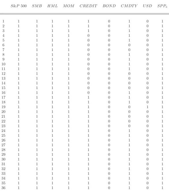
. For instance, focusing on the S&P 500, we obtain N S values close to zero, which means that this particular factor plays a significant role in explaining equity hedge fund returns. At the end, this procedure yields the 72 by 9 selection matrix S which is reported in the Appendix E. Each of the 72 rows of this matrix corresponds to a particular rolling period. Each element Sjt (j = 1, ..., m, t = 1, ..., 72) equals to one
if the jth factor satisfies the restriction imposed on the N S(j) criterion for the tth rolling period, and zero otherwise.
The selection matrix S highlights two important results concerning the risk exposures of the equity hedge fund returns.
i) The S&P 500 index, the Fama-French factors as well as the option-based factor SP Pa are always relevant.
ii) Factors such as U SD or CM DT Y seem to be irrelevant for most cases, while the CREDIT factor becomes relevant only at the beginning of 2000.
4.4 Dynamic linear regression analysis and replication
The two previous subsections help determine the risk dimension and identify the observed factors that are generated by (or are linear combinations of) the common latent factors estimated from the data. This subsection presents the linear regression analysis and the hedge fund replication methodology.
17
We try different critical values for N S(j) and obtain similar results. In particular, we allow for N S(j) critical value to vary from 10 to 20. The results reported in the next subsection consider a critical value equal to 15.
Hedge fund replication is used as a criterion for assessing the quality of the dynamic factor-based approach developed in this paper, as well as the benefits of dynamic factor selection mechanism. Note that our approach is similar to that of Hasanhodzic and Lo (2007). However, while they select in advance a set of observed factors and leave it unchanged through time, we allow for time-varying risk profile by using the factor selection methodology described in Sections 2 and 3.
We use a 37-month rolling window to estimate risk exposures for each fund i (i = 1, ..., N ) and construct an out-of-sample replicating portfolio. The first 36 months allow to i) estimate the risk dimension ht (i.e., the
number of the selected observed variables for a given rolling window); ii) select the relevant observed factors (G1, ..., Ght) and iii) perform the linear
regressions given below:
Ri,t−k = βi,t(1)G1,t−k+ ... + βi,t(ht)Ght,t−k+ ǫi,t−k,
f or k = 1, ..., 36, i = 1, ..., N, (4.1) subject to 1 = ht X j=1 βi,t(j), i = 1, ..., N.
In this equation, Ri,t−k denotes the return of fund i in t − k and βi,t(j) is the
fund’s i exposure to the jth factor. Beta coefficients are indexed by both i and t to reflect the fact that this process is repeated each month (using month t − 36 to t − 1 observations) for every fund i. To reflect that the number of observed factors considered for a given period is time-varying, ht
is also indexed by time. Thus, our approach is more general since account is taken not only of time-varying betas, but also of variability of hedge fund risk profile. In addition, selecting only the relevant factors eliminates noise
due to model overfitting and improves the ability of the regression model to explain the observed data. Hasanhodzic and Lo (2007) approach can then be seen as a particular case of our procedure, when risk profile is constant in time.
Following Hasanhodzic and Lo (2007), we omit the intercept, which forces the least squares algorithm to use the factor means to fit the mean of the fund, which is an important feature of replicating hedge fund expected re-turns with factor risk premia. In addition, we constraint the sum of beta coefficients to be one in order to get a portfolio interpretation of the weights.
The estimated regression coefficients bβ(ht)
i,t are then used as portfolio
weights for the ht observed factors. Hence, the replicated returns for the
fund i are equivalent to the fitted values bRi,t of the regression equation:
b
Ri,t = βbi,t(1)G1,t+ ... + bβ(hi,tt)Ght,t. (4.2)
The results obtained using our dynamic approach are compared with those of a naive replication strategy, which consists in including in the re-gression analysis the whole set of the observed factors. In this case, all the elements of the selecting matrix S are set to one and the number of factors h is constant over time. In this case, equations (4.1) and (4.2) include all the observed factors for each rolling window.
4.4.1 Empirical results
Applying the replication procedures exposed above, we get two equally-weighted replicating portfolios, called respectively the dynamic clone in-dex and the naive clone inin-dex, by averaging the returns of individual fund clones at each date. Both replicating portfolios are compared to the
equally-Dynamic Naive Equity
Clone Clone Hedge S&P 500 Index Index Index Index
Tracking Errors 1,23 1,55 -
-Annualized Return 8,06 6,85 9,50 0,02
Annualized SD 8.95 9.50 7,70 15,23
Table 1: Summary statistics for replication results (in percentage) using buy-and-hold and option-based factors.
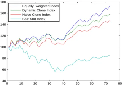
weighted equity hedge index built using the funds of our sample of data. Figure 4 plots the cumulative returns of the two clone indexes, the equally-weighted equity hedge index, as well as the S&P 500 for the whole replication period extending from January 2000 to December 2005 (72 months). The main summary statistics and the tracking errors of the replicating portfolios are reported in Table 1.
0 10 20 30 40 50 60 70 80 40 60 80 100 120 140 160 180 Equally−weighted Index Dynamic Clone Index Naive Clone Index S&P 500 Index
Figure 4: Cumulative returns of equally-weighted equity hedge fund portfo-lio, dynamic clone index, naive clone index, and the S&P 500 index.
Our dynamic replicating approach outperforms the naive one consisting of a static and ad hoc factor selection procedure. This highlights the benefits of taking into account the time-varying risk profile when analyzing hedge fund returns. In particular, we measure the benefits of using our dynamic approach instead of the naive one by the reduction of both replication risk (the tracking error), as well as the distance between the target and the clone average returns. When we look at average returns, the dynamic clone index outperforms the naive clone index. The annualized average return for the dynamic clone is 8, 06% with a volatility of 8, 95% against an average return of 6, 85% for the naive clone with a volatility of 9, 50%. The dynamic clone index has a lower tracking error (1, 23%) than the naive clone index (1, 55%). Thus, the dynamic replicating approach provides the best clone of the equity hedge index.
4.4.2 Additional results
We first study the influence of the risk dimension estimating criterion in the quality of replication. The dynamic clone index reported in Figure 4 is obtained using Bai and Ng (2002) IC2 criterion. In order to assess the
benefits of using these criterion, we perform the dynamic approach using the other criteria (see Subsection 2.2). The tracking errors are 1, 28% for the IC1 criterion and 1, 55% for IC3. Although the first alternative gives similar
performance, it is not the case for the second one18
, which highlights the importance of a good criterion selection.
Second, we analyze the impact of dynamic factor selection procedure on beta turnover. In the previous paragraph, we show that accounting for time-variability of hedge fund risk profile improves the quality of hedge fund
18
We also perform the dynamic replicating approach using the P C1, P C2 and P C3
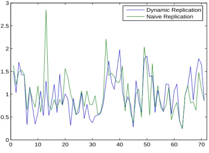
clone index. However, being time-dynamic may have a consequence in terms of beta turnover and other statistical properties of the different clones. At each replication date t (t = 1, ..., 72), we compute the turnover for a given individual hedge fund i (i = 1, ..., N ) as the sum of the absolute value of beta variations with respect to the previous period. Then, we take the average turnover across individual funds. Repeating this procedure for each rolling period, yields the time evolution of the average turnover, which is showed in Figure 5 for dynamic as well as naive approaches. The dynamic clone index outperformance as compared to the naive clone index is not necessarily due to higher fund turnover on average. Although turnover values are higher at individual fund level, they cancel each other when dealing with the index replication. 0 10 20 30 40 50 60 70 0 0.5 1 1.5 2 2.5 3 Dynamic Replication Naive Replication
Figure 5: Time evolution of average turnover across individual funds for dynamic and naive replication strategies.
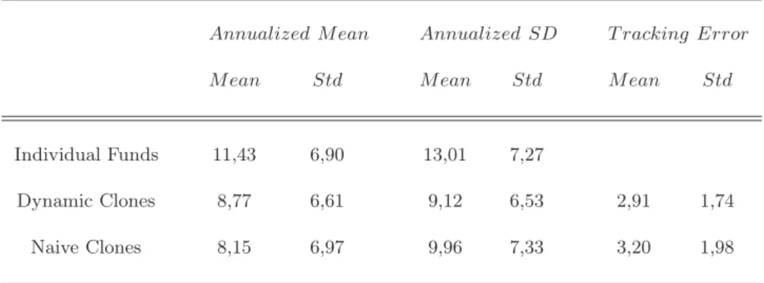
Third, we consider the replication quality at the individual fund level. Table 2 reports summary statistics for individual clones obtained by both
Annualized M ean Annualized SD T racking Error
M ean Std M ean Std M ean Std
Individual Funds 11,43 6,90 13,01 7,27
Dynamic Clones 8,77 6,61 9,12 6,53 2,91 1,74
Naive Clones 8,15 6,97 9,96 7,33 3,20 1,98
Table 2: Summary statistics for individual funds (in percentage). dynamic and naive replication approach. Columns 2 to 5 give the means and the standard deviations of the annualized average returns as well as annualized return volatility. Columns 6 and 7 report the means and standard deviations of individual clone tracking errors. The results show that the dynamic strategy outperforms the naive one. The tracking errors of the 3 worst fund clones in terms of replication quality are 9, 81%, 10, 32% and 11, 51% for the dynamic19
approach, and 11, 61%, 13, 65% and 14, 35% for the naive20
approach. On the other hand, the three best funds have tracking errors close to zero for both approaches. Hence, at the individual level, the dynamic clones behave better than the naive ones.
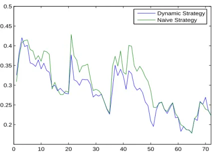
Finally, we study the difference between the two approaches in terms of equity exposure. Figure 6 shows the time evolution of the average market betas across individual funds. At each replication date t we estimate market factor loadings of individual funds and take their average. Repeating this procedure 72 times yields the average beta time dynamics. The market beta is (on average) more stable when using the dynamic approach, which can be explained by a lower selection error due to the allowance for dynamic risk
19
The tracking errors for the naive counterparts of these three worst dynamic clones are 13, 65%, 10, 97% and 11, 67%, respectively.
20
The tracking errors for the dynamic counterparts of these three worst naive clones are 9, 24%, 9, 81% and 9, 51%, respectively.
profile. 0 10 20 30 40 50 60 70 0.2 0.25 0.3 0.35 0.4 0.45 0.5 Dynamic Strategy Naive Strategy
Figure 6: Time evolution of average market betas across individual funds for dynamic and naive procedures.
5
Concluding remarks
In this paper, we link a new market practice − hedge fund replication, to some useful and well known financial theory − factor modelling of equity returns. We get a deeper comprehension of the underlying factor structure that drives the covariations of equity hedge fund returns, using individual fund returns instead of index performances. Recent asymptotic theories for factor selection ensure good finite sample properties for large N and moderately large T , which is clearly more in line with the dynamic factor selection objective we aim at.
This approach allows us to obtain several empirical results. First, equity hedge funds belonging to the HFR database exhibit a simple 2-3 factor struc-ture. While the first factor behaves closely with the equity market index,
the second one is often more difficult to understand and illustrates the style rotation employed by hedge fund managers. Second, the economic interpre-tation of the risk factors allows building replicating portfolios as they are proposed by practitioners. Our results highlight the interest of taking into account time-varying risk profile in the replication procedure at aggregated level but also at the individual one. The dynamic approach outperforms the naive one, which consists of a static and ad hoc factor selection procedure.
References
Agarwal, V. and Naik, N. Y. (2001). Characterizing Hedge Fund Risks with Buy-and-Hold and Option-Based Strategies. Working Paper.
Agarwal, V. and Naik, N. Y. (2004). Risks and Portfolio Decisions Involving Hedge Funds. The Review of Financial Studies, 17(1):63–98.
Amin, G. S. and Kat, H. M. (2003). Hedge Fund Performance 1990-2000:
Do the Money Machines Really Add Value? Journal of Financial and
Quantitative Analysis, 38(2):251–274.
Anderson1, T. W. (1984). An Introduction to Multivariate Statistical Anal-ysis. New York: Wiley.
Asness, C., Krail, R., and Liew, J. (2001). Do Hedge Funds Hedge? Journal of Portfolio Management, 28:6–19.
Bai, J. and Ng, S. (2002). Determining the Number of Factors in Approxi-mate Factor Models. Econometrica, 70:191–221.
Bai, J. and Ng, S. (2003). Inferential Theory for Factor Models of Large Dimensions. Econometrica, 71:135–171.
Bai, J. and Ng, S. (2006). Evaluating Latent and Observed Factors in Macroeconomics and Finance. Journal of Econometrics, 131:507–537. Black, F. (1972). Capital Market Equilibrium with Restricted Borrowing.
Journal of Business, 45:444–454.
Breeden, D. T., Gibbons, M. R., and Litzenberger, R. H. (1989). Empirical Tests of the Consumption-Oriented CAPM. Journal of Finance, 44:231– 262.
Carhart, M. (1997). On Persistence in Mutual Fund Performance. Journal of Finance, 52(1):57–92.
Chamberlain, G. and Rothschild, M. (1983). Arbitrage, Factor Structure and Mean-Variance Analysis in Large Asset Markets. Econometrica, 51:1305– 1324.
Chan, N., Getmansky, M., Haas, S. M., and Lo, A. W. (2005). Systemic Risk and Hedge Funds. Working Paper.
Chen, N., Roll, R., and Ross, S. (1986). Economic Forces and the Stock Market. Journal of Business, 59:383–403.
Connor, G. and Korajczyk, R. A. (1986). Performance Measurement with the APT. Journal of Financial Economics, 15:373–394.
Connor, G. and Korajczyk, R. A. (1988). Risk and Return in an Equilib-rium APT: Application to a New Test Methodology. Journal of Financial Economics, 21:255–289.
Connor, G. and Korajczyk, R. A. (1993). A Test for the Number of Factors in an Approximate Factor Model. Journal of Finance, 48:1263–1291. Dhrymes, P., Friend, I., and Gultekin, M. (1984). A Critical Re-Examination
of the Empirical Evidence on the Arbitrage Pricing Theory. Journal of Finance, 39:323–346.
Fama, E. F. and French, K. R. (1993). Common Risk Factors in the Returns on Stocks and Bonds. Journal of Financial Economics, 33(1):3–56. Fung, W. and Hsieh, D. A. (1997a). Empirical Characteristics of Dynamic
Fung, W. and Hsieh, D. A. (1997b). Investment Style and Survivorship Biais in the Returns of the CTAs: The Information Content of Track Records. Fung, W. and Hsieh, D. A. (2000). Performance Characteristics of Hedge
Funds and Commodity Funds: Natural vs. Spurious Biases. Journal of Financial and Quantitative Analysis, 35:291–307.
Fung, W. and Hsieh, D. A. (2001). The Risk in Hedge Fund Strategies: Theory and Evidence from Trend Followers. The Review of Financial Studies, 14(2):313–341.
Fung, W. and Hsieh, D. A. (2002). Asset-Based Style Factors for Hedge Funds. Financial Analysis Journal, 58:16–27.
Fung, W. and Hsieh, D. A. (2004). Extracting Portable Alphas from Equity Long-Short Hedge Funds. Journal of Investment Management, 2(4):1–19. Hasanhodzic, J. and Lo, A. W. (2007). Can Hedge-Funds Be Replicated.
Journal of Investment Management, 5(2):5–45.
Lehman, B. and Modest, D. (1988). The Empirical Foundations of the Ar-bitrage Pricing Theory. Journal of Financial Economics, 21:213–254. Liang, B. (2000). Hedge Funds: The Living and the Dead. Journal of
Financial and Quantitative Analysis, 35:309–326.
Lintner, J. (1965). The Valuation of Risky Assets and the Selection of Risky Investment in Stock Portfolios and Capital Budgets. Review of Economics and Statistics, 47:13–37.
Mitchell, M. and Pulvino, T. (2001). Characteristics of Risk and Return in Risk Arbitrage. Journal of Finance, 56(6):2135–2175.
Roll, R. and Ross, S. A. (1980). An Empirical Investigation of the Arbitrage Pricing Theory. Journal of Finance, 35:1073–1103.
Ross, S. A. (1976). The Arbitrage Theory of Capital Asset Pricing. Journal of Economic Theory, 13(3):341–360.
Shanken, J. (1992). On the Estimation of Beta Pricing Models. The Review of Financial Studies, 5:1–33.
Sharpe, W. F. (1964). Capital Asset Prices: A Theory of Market Equilibrium Under Conditions of Risk. Journal of Finance, 19:425–442.
Appendices
A
Bai and Ng (2002) assumptions for approximate
factor structure
To allow for some cross and serial correlation as well as heteroskedasticity in the idiosyncratic components, Bai and Ng (2002) make the following set of assumptions:
Assumptions Time and cross-section dependence and heteroskedasticity:
There exists a positive constant M < ∞, such that for all N and T , 1. E(eit) = 0, E|eit|8 ≤ M;
2. E(e′se′t/N ) = E(N−1Pi=1N eiseit) = γN(s, t), |γN(s, s)| ≤ M for all s,
and T−1PTs=1PTt=1|γN(s, t)| ≤ M;
3. E(eitejt) = τij,t with |τij,t| ≤ |τij| for some τij and for all t;
in addition, N−1PN i=1
PN
j=1|τij| ≤ M;
4. E(eitejs) = τij,ts and (N T )−1PNi=1
PN j=1 PT t=1 PT s=1|τij,ts| ≤ M;
5. for every (t, s), E|N−1/2PN
i=1[eiseit− E(eiseit)]|4 ≤ M.
Given Assumption 1, the remaining assumptions presented above are easily satisfied if the eit are independent for all i and t. Assumptions 2
and 3 respectively allow for limited time-series and cross-section dependence in the idiosyncratic components. Heteroscedasticity in both dimensions is also allowed (Assumption 4). In addition the authors allow for some weak dependence between factors and the idiosyncratic errors, which is formalized by: E 1 Nk 1 √ T T X t=1 Fteitk2 ! ≤ c.
B
Determining the number of latent factors: Monte
Carlo simulations
Although asymptotically equivalent, the IC criteria do not have the same finite sample properties [see Bai and Ng (2002)]. We perform Monte Carlo simulations to assess the finite sample properties of the three information panel criteria given in (2.5). In particular, we are interested in cases of large N but moderately large T . As in Bai and Ng (2002), we simulate data from the following model21
: Xit= r X j=1 λijFjt+ √ θeit = cit+ √ θeit, (B.1)
where the idiosyncratic errors are generated by the following equation in order to allow for serial and cross-section correlation:
eit= ρeit−1+ νit+ J
X
j6=0,j6=−J
βνi−jt. (B.2)
In this equation, ρ and β represent serial and cross-section correlation pa-rameters, respectively, J is the number of the cross-correlated idiosyncratic components with θ being their variance.
The factors are T × r matrices of N(0, 1) variables and the factor loading are N (0, 1) variables. Hence, the common component of Xit, denoted by
cit , has variance r. Our model assumes that the idiosyncratic component
has the same variance22
as the common component (i.e., θ = r). We set ρ = 0.50, β = 0.20 and J = max [N/20, 10].
21
All computations are performed using Matlab. The programs used for Monte Carlo simulations and test statistic computations are available upon request.
22
Bai and Ng (2002) also performed simulations allowing for the variance of the id-iosyncratic component to be larger than that of the common component and yield similar results for the finite sample properties of their criteria.
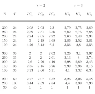
We consider thirteen configurations of the data. The first five simulate plausible asset pricing applications with two years of monthly data (T = 24) for 100 to 300 series of asset returns. We then increase T to 36 months. The last three configurations are more general and are used to recall the results obtained by Bai and Ng (2002). For each data configuration, we use the procedure exposed in section 2 in order to estimate the number of factors br and repeat the exercice 1000 times. Table 3 shows the test results, averaged across 1000 simulations, for r = 2 (columns 3 to 5) and r = 3 (columns 6 to 8). Three main remarks can be drawn.
i) The IC2 criteria outperforms (on average) IC1 and IC3;
ii) For small T (T = 24), the three criteria lose (on average) their precision, even when N is large. For T = 36, they do better in inferring the number of common factors used to generate the data;
iii) When T and N are both small, the criteria do not perform efficiently in inferring the appropriate number of factors. For example, for N = 30 and T = 40 both sets of criteria overestimate r.
r= 2 r= 3 N T IC1 IC2 IC3 IC1 IC2 IC3 300 24 2,08 2,02 2,3 2,79 2,75 2,89 260 24 2,59 2,31 3,56 2,82 2,75 2,88 200 24 2,24 2,05 2,92 2,63 2,48 2,94 150 24 3 2,48 4,68 2,86 2,52 3,81 100 24 4,26 3,42 6,2 3,56 2,8 5,55 300 36 2 2 2,02 3,26 3,1 3,97 260 36 2 2 2,01 3,13 3 3,74 200 36 2,6 2,29 4,19 2,98 2,89 3,45 150 36 2,35 2,15 3,76 2,99 2,96 3,16 100 36 3,33 2,66 5,31 4,1 3,32 6,34 200 60 2,27 2,07 4,52 3,26 3,06 5,48 200 100 3,44 2,39 7,84 4,4 3,39 7,98 30 40 1 1 1 1 1 1
Table 3: Simulation results for IC criteria.
C
Matching the latent factors with the observed
variables: Monte Carlo simulations
We perform Monte Carlo simulations in order to asses the finite sample prop-erties of the asymptotic tests N S(j) and R2(j) using the same data configu-rations as in appendix B.1 (T = 24, 36 and N = 100, 150, 200, 250, 300). We assume Fkt ∼ N (0, 1), k = 1, ..., r and eit ∼ N (0, σ2e(i)), where eit is
uncorrelated with ejt for i 6= j, i, j = 1, ..., N. The factor loadings are
standard normal, i.e. λij ∼ N (0, 1), j = 1, ..., r, i = 1, ..., N . The data are generated as Xit = λ
′
itFt+ eit. We assume that there are r = 2
fac-tors and that this is known. The data are standardized to have mean zero and unit variance prior to the estimation of the factors by the method of asymptotic principal components.
vector of weights, and ǫjt∼ σǫ(j)N (0, var(δj′Ft)). As in Bai and Ng (2006),
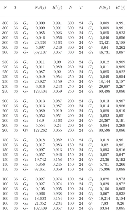
we test m = 7 observed variables parameterized as given in table 4:
J 1 2 3 4 5 6 7
δj1 1 1 1 1 1 1 0
δj2 1 0 0 1 0 1 0
σǫ 0 0 0.2 0.2 2 2 1
Table 4: Parameters for Gjt simulation.
The first two factors, G1t and G2t, are exact factors since σǫ = 0.
Fac-tors three to six are linear combinations of the two latent facFac-tors but are contaminated by errors. The variance of this error is small relative to the variations of the latent factors for G3t and G4t, but is large for G5tand G6t.
Finally, G7t is an irrelevant factor as it is simply a random variable N (0, 1).
The Monte Carlo simulation results are reported in Table 5. The test statistics are averaged over 1000 simulations. The N S(j) and R2(j) statistics reinforce the previous result. When the observed factors are contaminated by errors, Table 5 shows that the higher the variance of this error, the worse is the efficiency of the tests considered here. Finally, the test precision is higher for T = 36 than for T = 24.
N T N S(j) R2 (j) N T N S(j) R2 (j) 300 36 G1 0,009 0,991 300 24 G1 0,009 0,991 300 36 G2 0,009 0,991 300 24 G2 0,009 0,991 300 36 G3 0,085 0,923 300 24 G3 0,085 0,923 300 36 G4 0,046 0,956 300 24 G4 0,046 0,956 300 36 G5 20,338 0,163 300 24 G5 33,421 0,188 300 36 G6 5,697 0,246 300 24 G6 8,64 0,262 300 36 G7 567,107 0,057 300 24 G7 46,731 0,087 250 36 G1 0,011 0,99 250 24 G1 0,012 0,989 250 36 G2 0,011 0,989 250 24 G2 0,011 0,989 250 36 G3 0,087 0,92 250 24 G3 0,085 0,922 250 36 G4 0,049 0,954 250 24 G4 0,049 0,954 250 36 G5 20,927 0,159 250 24 G5 18,144 0,187 250 36 G6 6,616 0,243 250 24 G6 29,687 0,267 250 36 G7 128,404 0,059 250 24 G7 60,498 0,086 200 36 G1 0,013 0,987 200 24 G1 0,013 0,987 200 36 G2 0,013 0,987 200 24 G2 0,014 0,986 200 36 G3 0,089 0,919 200 24 G3 0,089 0,919 200 36 G4 0,052 0,951 200 24 G4 0,052 0,951 200 36 G5 18,9 0,163 200 24 G5 28,367 0,191 200 36 G6 5,554 0,24 200 24 G6 6,084 0,269 200 36 G7 127,262 0,055 200 24 G7 80,598 0,086 150 36 G1 0,018 0,982 150 24 G1 0,019 0,981 150 36 G2 0,017 0,983 150 24 G2 0,02 0,981 150 36 G3 0,097 0,913 150 24 G3 0,093 0,916 150 36 G4 0,057 0,946 150 24 G4 0,057 0,947 150 36 G5 19,742 0,158 150 24 G5 23,36 0,192 150 36 G6 5,856 0,245 150 24 G6 5,701 0,266 150 36 G7 97,851 0,059 150 24 G7 75,996 0,088 100 36 G1 0,027 0,974 100 24 G1 0,028 0,973 100 36 G2 0,027 0,974 100 24 G2 0,029 0,972 100 36 G3 0,105 0,905 100 24 G3 0,106 0,905 100 36 G4 0,066 0,938 100 24 G4 0,067 0,938 100 36 G5 18,603 0,154 100 24 G5 19,214 0,184 100 36 G6 21,352 0,234 100 24 G6 7,83 0,26 100 36 G7 102,409 0,057 100 24 G7 83,84 0,085
Table 5: Simulation results: Matching the observed variables to latent fac-tors.
D
Data description
Strategy Fund Number
1 Convertible Arbitrage 109
2 Distressed Securities 127
3 Emerging Markets 269
4 Equity Hedge 1232
5 Equity Market Neutral 282
6 Equity Non-Hedge 146 7 Event-Driven 225 8 Fixed Income 310 9 Foreign Exchange 68 10 Fund of Funds 2011 11 Macro 277 12 Managed Futures 337 13 Market Timing 25 14 Merger Arbitrage 46
15 Relative Value Arbitrage 268
16 Sector 279
17 Short Selling 23
Total 6034
Table 6: Fund repartition by strategy for the HFR Database in December 2005.
S&P 500 SM B HM L M OM CREDIT BON D CM DT Y U SD SP Pa 1 1 1 1 1 1 0 1 0 1 2 1 1 1 1 1 0 1 0 1 3 1 1 1 1 1 0 1 0 1 4 1 1 1 1 0 0 1 0 1 5 1 1 1 1 0 0 1 0 1 6 1 1 1 1 0 0 0 0 1 7 1 1 1 1 0 0 0 0 1 8 1 1 1 1 0 0 1 0 1 9 1 1 1 1 0 0 1 0 1 10 1 1 1 1 0 0 1 0 1 11 1 1 1 1 0 0 1 0 1 12 1 1 1 1 0 0 0 0 1 13 1 1 1 1 0 0 0 0 1 14 1 1 1 1 0 0 0 0 1 15 1 1 1 1 0 0 0 0 1 16 1 1 1 1 0 0 1 0 1 17 1 1 1 1 1 0 1 0 1 18 1 1 1 1 1 0 1 0 1 19 1 1 1 1 1 0 0 1 1 20 1 1 1 1 1 0 0 0 1 21 1 1 1 1 1 0 0 0 1 22 1 1 1 1 1 0 0 0 1 23 1 1 1 1 1 0 0 0 1 24 1 1 1 1 1 0 1 0 1 25 1 1 1 1 1 0 1 0 1 26 1 1 1 1 1 0 1 0 1 27 1 1 1 1 1 0 1 0 1 28 1 1 1 1 1 0 1 0 1 29 1 1 1 1 1 0 1 0 1 30 1 1 1 1 1 0 1 0 1 31 1 1 1 1 1 0 1 0 1 32 1 1 1 1 1 0 1 0 1 33 1 1 1 1 1 0 1 0 1 34 1 1 1 1 1 0 1 0 1 35 1 1 1 1 1 0 1 0 1 36 1 1 1 1 1 0 1 0 1
S&P 500 SM B HM L M OM CREDIT BON D CM DT Y U SD SP Pa 37 1 1 1 1 1 0 1 0 1 38 1 1 1 1 1 0 1 0 1 39 1 1 1 1 1 0 0 0 1 40 1 1 1 1 1 1 0 1 1 41 1 1 1 1 1 0 1 0 1 42 1 1 1 1 1 0 1 0 1 43 1 1 1 1 1 0 1 0 1 44 1 1 1 1 1 0 1 0 1 45 1 1 1 1 1 0 0 0 1 46 1 1 1 1 1 0 0 0 1 47 1 1 1 1 1 1 0 0 1 48 1 1 1 1 1 1 0 0 1 49 1 1 1 1 1 1 0 0 1 50 1 1 1 1 1 1 0 0 1 51 1 1 1 1 1 0 0 0 1 52 1 1 1 1 1 0 0 1 1 53 1 1 1 1 1 0 1 1 1 54 1 1 1 1 1 0 1 1 1 55 1 1 1 1 1 0 1 1 1 56 1 1 1 1 1 0 1 1 1 57 1 1 1 1 1 0 1 1 1 58 1 1 1 1 1 1 1 1 1 59 1 1 1 1 1 1 1 0 1 60 1 1 1 1 1 1 1 1 1 61 1 1 1 1 1 1 0 0 1 62 1 1 1 1 1 1 1 1 1 63 1 1 1 1 1 1 1 1 1 64 1 1 1 1 1 1 1 1 1 65 1 1 1 1 1 1 1 1 1 66 1 1 1 1 1 1 1 1 1 67 1 1 1 1 1 0 1 1 1 68 1 1 1 1 1 0 1 1 1 69 1 1 1 1 1 1 1 1 1 70 1 1 1 1 1 0 1 0 1 71 1 1 1 1 1 1 1 1 1 72 1 1 1 1 1 1 1 1 1